Coding Theory and Projective Spaces Natalia Silberstein

Coding Theory and

arXiv:0805.3528v2 [cs.IT] 8 Sep 2011

Projective Spaces

Natalia Silberstein

Coding Theory and Projective Spaces

Research Thesis

In Partial Fulfillment of the Requirements for the Degree of Doctor of Philosophy

Natalia Silberstein

Submitted to the Senate of the Technion — Israel Institute of Technology Elul 5771

Haifa

September 2011

This Research Thesis was done under the supervision of Prof. Tuvi Etzion in the Department of Computer Science.

The Generous Financial Help Of The Technion, Israeli Science Foundation, and Neaman Foundation Is Gratefully Acknowledged

List of Publications Journal Publications 1. T. Etzion and N. Silberstein, “Error-Correcting Codes in Projective Spaces Via Rank-Metric Codes and Ferrers Diagrams”, IEEE Transactions on Information Theory, Vol. 55, No. 7, pp. 2909–2919, July 2009. 2. N. Silberstein and T. Etzion, “Enumerative Coding for Grassmannian Space”, IEEE Transactions on Information Theory, Vol. 57, No. 1, pp. 365 - 374, January 2011. 3. N. Silberstein and T. Etzion, “Large Constant Dimension Codes and Lexicodes”, Advances in Mathematics of Communications (AMC), vol. 5, No. 2, pp. 177 - 189, 2011. 4. T. Etzion and N. Silberstein, “Codes and Designs Related to Lifted MRD Codes”, submitted to IEEE Transactions on Information Theory.

Conference Publications 1. T. Etzion and N. Silberstein, “Construction of Error-Correcting Codes For Random Network Coding”, in IEEE 25th Convention of Electrical & Electronics Engineers in Israel (IEEEI 2008), pp. 70 - 74, Eilat, Israel, December 2008. 2. N. Silberstein and T. Etzion, “Enumerative Encoding in the Grassmannian Space”, in 2009 IEEE Information Theory Workshop (ITW 2009), pp. 544 - 548, Taormina, Sicily, October 2009. 3. N. Silberstein and T. Etzion, “Large Constant Dimension Codes and Lexicodes”, in Algebraic Combinatorics and Applications (ALCOMA 10), Thurnau, Germany, April 2010. 4. N. Silberstein and T. Etzion, “Codes and Designs Related to Lifted MRD Codes”, in IEEE International Symposium on Information Theory (ISIT 2011), pp. 2199 2203, Saint Petersburg, Russia, July-August 2011.

Contents Abstract

1

Abbreviations and Notations

3

1 Introduction

5

1.1

Codes in Projective Space . . . . . . . . . . . . . . . . . . . . . . . . . . . .

5

1.2

Random Network Coding . . . . . . . . . . . . . . . . . . . . . . . . . . . .

6

1.2.1

Errors and Erasures Correction in Random Network Coding . . . . .

6

1.3

Rank-Metric Codes . . . . . . . . . . . . . . . . . . . . . . . . . . . . . . . .

8

1.4

Related Work . . . . . . . . . . . . . . . . . . . . . . . . . . . . . . . . . . .

9

1.4.1

Bounds . . . . . . . . . . . . . . . . . . . . . . . . . . . . . . . . . .

9

1.4.2

Constructions of Codes . . . . . . . . . . . . . . . . . . . . . . . . . 12

1.5

Organization of This Work

. . . . . . . . . . . . . . . . . . . . . . . . . . . 14

2 Representations of Subspaces and Distance Computation 2.1

2.2

Representations of Subspaces . . . . . . . . . . . . . . . . . . . . . . . . . . 16 2.1.1

Reduced Row Echelon Form Representation . . . . . . . . . . . . . . 16

2.1.2

Ferrers Tableaux Form Representation . . . . . . . . . . . . . . . . . 18

2.1.3

Extended Representation . . . . . . . . . . . . . . . . . . . . . . . . 21

Distance Computation . . . . . . . . . . . . . . . . . . . . . . . . . . . . . . 22

3 Codes and Designs Related to Lifted MRD Codes 3.1

3.2

16

26

Lifted MRD Codes and Transversal Designs . . . . . . . . . . . . . . . . . . 27 3.1.1

Properties of Lifted MRD Codes . . . . . . . . . . . . . . . . . . . . 27

3.1.2

Transversal Designs from Lifted MRD Codes . . . . . . . . . . . . . 30

Linear Codes Derived from Lifted MRD Codes . . . . . . . . . . . . . . . . 32 i

3.2.1

Parameters of Linear Codes Derived from CMRD . . . . . . . . . . . 33

3.2.2

LDPC Codes Derived from CMRD

. . . . . . . . . . . . . . . . . . . 39

4 New Bounds and Constructions for Codes in Projective Space 4.1

4.2

4.3

43

Multilevel Construction via Ferrers Diagrams Rank-Metric Codes . . . . . . 43 4.1.1

Ferrers Diagram Rank-Metric Codes . . . . . . . . . . . . . . . . . . 44

4.1.2

Lifted Ferrers Diagram Rank-Metric Codes . . . . . . . . . . . . . . 49

4.1.3

Multilevel Construction . . . . . . . . . . . . . . . . . . . . . . . . . 51

4.1.4

Code Parameters . . . . . . . . . . . . . . . . . . . . . . . . . . . . . 53

4.1.5

Decoding . . . . . . . . . . . . . . . . . . . . . . . . . . . . . . . . . 54

Bounds and Constructions for Constant Dimension Codes that Contain CMRD 56 4.2.1

Upper Bounds for Constant Dimension Codes . . . . . . . . . . . . . 57

4.2.2

Upper Bounds for Codes which Contain Lifted MRD Codes . . . . . 59

4.2.3

Construction for (n, M, 4, 3)q Codes . . . . . . . . . . . . . . . . . . 61

4.2.4

Construction for (8, M, 4, 4)q Codes

. . . . . . . . . . . . . . . . . . 66

Error-Correcting Projective Space Codes . . . . . . . . . . . . . . . . . . . . 69 4.3.1

Punctured Codes . . . . . . . . . . . . . . . . . . . . . . . . . . . . . 70

4.3.2

Code Parameters . . . . . . . . . . . . . . . . . . . . . . . . . . . . . 72

4.3.3

Decoding . . . . . . . . . . . . . . . . . . . . . . . . . . . . . . . . . 73

5 Enumerative Coding and Lexicodes in Grassmannian 5.1

Lexicographic Order for Grassmannian . . . . . . . . . . . . . . . . . . . . . 77 5.1.1 5.1.2

5.2

Order for Gq(n, k) Based on Extended Representation . . . . . . . . 77

Order for Gq(n, k) Based on Ferrers Tableaux Form . . . . . . . . . . 78

Enumerative Coding for Grassmannian . . . . . . . . . . . . . . . . . . . . . 79 5.2.1 5.2.2 5.2.3

5.3

76

Enumerative Coding for Gq(n, k) Based on Extended Representation

Enumerative Coding for Gq(n, k) Based on Ferrers Tableaux Form

Combination of the Coding Techniques

80

. 87

. . . . . . . . . . . . . . . . 94

Constant Dimension Lexicodes . . . . . . . . . . . . . . . . . . . . . . . . . 97 5.3.1

Analysis of Constant Dimension Codes . . . . . . . . . . . . . . . . . 97

5.3.2

Search for Constant Dimension Lexicodes . . . . . . . . . . . . . . . 101

6 Conclusion and Open Problems

106

Bibliography

108

ii

List of Figures 1.1

Network coding example. Max-flow is attainable only through the mixing of information at intermediate nodes. . . . . . . . . . . . . . . . . . . . . . .

iii

7

List of Tables 3.1

LDPC codes from CMRD vs. LDPC codes from finite geometries . . . . . . 40

4.1

The (8, 4573, 4, 4)2 code C . . . . . . . . . . . . . . . . . . . . . . . . . . . . 53

4.2

CML vs. CMRD . . . . . . . . . . . . . . . . . . . . . . . . . . . . . . . . . . 54

4.3

Qs (q) . . . . . . . . . . . . . . . . . . . . . . . . . . . . . . . . . . . . . . . 58

4.4

Q′δ−1 (q) for k = 3

. . . . . . . . . . . . . . . . . . . . . . . . . . . . . . . . 58

4.5

Q′δ−1 (q)

. . . . . . . . . . . . . . . . . . . . . . . . . . . . . . . . 58

for k = 4

|CML | upper bound

4.6

Lower bound on

4.7

The size of new codes vs. the previously known codes and the upper

. . . . . . . . . . . . . . . . . . . . . . . . . . . 59

bound (4.3) . . . . . . . . . . . . . . . . . . . . . . . . . . . . . . . . . . . . 66 4.8 4.9

Lower bounds on ratio between |Cnew | and the bound in (4.3)

. . . . . . . 66

The size of new codes vs. previously known codes and bound (4.3) . . . . . 68

4.10 The punctured (7, 573, 3)q code C′Q,v . . . . . . . . . . . . . . . . . . . . . . 71 5.1

Clex vs. CM L in G2 (8, 4) with dS = 4 . . . . . . . . . . . . . . . . . . . . . . 102

iv

Abstract The projective space of order n over a finite field Fq , denoted by Pq (n), is a set of all

subspaces of the vector space Fnq . The projective space is a metric space with the distance

function ds (X, Y ) = dim(X) + dim(Y ) − 2dim(X ∩ Y ), for all X, Y ∈ Pq (n). A code in the

projective space is a subset of Pq (n). Coding in the projective space has received recently

a lot of attention due to its application in random network coding.

If the dimension of each codeword is restricted to a fixed nonnegative integer k ≤ n,

then the code forms a subset of a Grassmannian, which is the set of all k-dimensional subspaces of Fnq , denoted by Gq(n, k). Such a code is called a constant dimension code.

Constant dimension codes in the projective space are analogous to constant weight codes in the Hamming space.

In this work, we consider error-correcting codes in the projective space, focusing mainly on constant dimension codes. We start with the different representations of subspaces in Pq(n). These representa-

tions involve matrices in reduced row echelon form, associated binary vectors, and Ferrers diagrams. Based on these representations, we provide a new formula for the computation of the distance between any two subspaces in the projective space. We examine lifted maximum rank distance (MRD) codes, which are nearly optimal constant dimension codes. We prove that a lifted MRD code can be represented in such a way that it forms a block design known as a transversal design. A slightly different representation of this design makes it similar to a q-analog of transversal design. The incidence matrix of the transversal design derived from a lifted MRD code can be viewed as a parity-check matrix of a linear code in the Hamming space. We find the properties of these codes which can be viewed also as LDPC codes. We present new bounds and constructions for constant dimension codes. First, we present a multilevel construction for constant dimension codes, which can be viewed as a 1

generalization of a lifted MRD codes construction. This construction is based on a new type of rank-metric codes, called Ferrers diagram rank-metric codes. We provide an upper bound on the size of Ferrers diagram rank-metric codes and present a construction of codes that attain this bound. Then we derive upper bounds on the size of constant dimension codes which contain the lifted MRD code, and provide a construction for two families of codes, that attain these upper bounds. Most of the codes obtained by these constructions are the largest known constant dimension codes. We generalize the well-known concept of a punctured code for a code in the projective space to obtain large codes which are not constant dimension. We present efficient enumerative encoding and decoding techniques for the Grassmannian. These coding techniques are based on two different lexicographic orders for the Grassmannian induced by different representations of k-dimensional subspaces of Fnq . Finally we describe a search method for constant dimension lexicodes. Some of the codes obtained by this search are the largest known constant dimension codes with their parameters.

2

Abbreviations and Notations Fq

—

a finite field of size q

Pq(n)

—

the projective space of order n

Gq(n, k)

—

the Grassmannian

—

the subspace distance

dR (·, ·)

—

the rank distance

—

the Hamming distance

C

—

a code in the projective space

CMRD

—

the lifted MRD code

C

—

a rank-metric code

C

—

a code in the Hamming space

RREF

—

reduced row echelon form

RE(X)

—

a subspace X in RREF

v(X)

—

the identifying vector of a subspace X

FE(X)

—

the Ferrers echelon form of a subspace X

F

—

Ferrers diagram

—

the Ferrers diagram of a subspace X

F(X)

—

the Ferrers taubleux form of a subspace X

dS (·, ·)

dH (·, ·)

FX

EXT(X)  

—

the extended representation of a subspace X

—

the q-ary Gaussian coefficient

TDλ (t, k, m)

—

a transversal design of blocksize k, groupsize m,

n k

q

strength t and index λ TDλ (k, m)

—

a transversal design TDλ (2, k, m)

STDq (t, k, m)

—

a subspace transversal design of block dimension k, groupsize q m and strength t

OAλ (N, k, s, t)

—

an N × k orthogonal array with s levels, strength t, and index λ 3

4

Chapter 1

Introduction 1.1

Codes in Projective Space

Let (M, d) be a metric space, where M is a finite set, and d is a metric defined on M . A code C in M is a collection of elements of M ; it has minimum distance d, if for each two different elements A, B ∈ M , d(A, B) ≥ d. Let Fq be the finite field of size q. The projective space of order n over Fq , denoted by Pq(n), is the set of all subspaces of the vector space Fnq . Given a nonnegative integer k ≤ n, the set of all k-dimensional subspaces of Fnq forms the Grassmannian space (Grassmannian S in short) over Fq , which is denoted by Gq(n, k). Thus, Pq(n) = 0≤k≤n Gq(n, k). It is well

known that

|Gq(n, k)| = where



n k





n k



= q

k−1 Y i=0

q n−i − 1 , q k−i − 1

is the q-ary Gaussian coefficient. The projective space and the Grassmannian q

are metric spaces with the distance function, called subspace distance, defined by
def dS (X,Y ) = dim X + dim Y − 2 dim X ∩Y ,

(1.1)

for any two subspaces X and Y in Pq(n). A subset C of the projective space is called an (n, M, dS )q code in projective space if it has size M and minimum distance dS . If an (n, M, dS )q code C is contained in Gq(n, k) for some k, we say that C is an (n, M, dS , k)q constant dimension code. The (n, M, d)q , respectively (n, M, d, k)q , codes in projective space are akin to the familiar 5

codes in the Hamming space, respectively constant-weight codes in the Johnson space, where the Hamming distance serves as the metric. Koetter and Kschischang [43] showed that codes in Pq(n) are precisely what is needed

for error-correction in random network coding [11, 12]. This is the motivation to explore error-correcting codes in Pq(n).

1.2

Random Network Coding

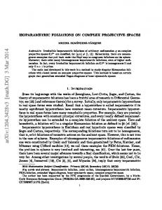
A network is a directed graph, where the edges represent pathways for information. Using the max-flow min-cut theorem, one can calculate the maximum amount of information that can be pushed through this network between any two graph nodes. It was shown that simple forwarding of information between the nodes is not capable of attaining the max-flow value. Rather, by allowing mixing of data at intermediate network nodes this value can be achieved. Such encoding is referred to as network coding [2, 30, 31]. In the example in Figure 1.1, two sources having access to bits A and B at a rate of one bit per unit time, have to communicate these bits to two sinks, so that both sinks receive both bits per unit time. All links have a capacity of one bit per unit time. The network problem can be satisfied with the transmissions specified in the example but cannot be satisfied with only forwarding of bits at intermediate packet nodes.

1.2.1

Errors and Erasures Correction in Random Network Coding

Now we describe the network coding model proposed by Koetter and Kschischang [43]. Consider a communication between a single source and a single destination node. During each generation, the source node injects m packets x1 , x2 , . . . , xm ∈ Fnq into the network. When an intermediate node has a transmission opportunity, it creates an outgoing packet as a random Fq -linear combination of the incoming packets. The destination node collects such randomly generated packets y1 , y2 , . . . , yN ∈ Fnq , and tries to recover the injected

packets into the network. The matrix form representation of the transmission model is Y = HX,

where H is a random N × m matrix, corresponding to the overall linear transformation

applied to the network, X is the m × n matrix whose rows are the transmitted packets,

and Y is the N × n matrix whose rows are the received packets. Note, that there is no 6

Figure 1.1: Network coding example. Max-flow is attainable only through the mixing of information at intermediate nodes.

assumption here that the network operates synchronously or without delay or that the network is acyclic. If we consider the extension of this model by incorporation of T packet errors e1 , e2 , . . . , eT then the matrix form representation of the transmission model is given by Y = HX + GE, where X, Y , and E are m × n, N × n, and T × n matrices, respectively, whose rows

represent the transmitted, received, and erroneous packets, respectively, and H and G are corresponding random N × m and N × T matrices induced by linear network coding.

Note, that the only property of the matrix X that is preserved under the unknown

linear transformation applied by random network coding, is its row space. Therefore, the information can be encoded by the choice of the vector space spanned by the rows of X, and not by the choice of X. Thus, the input and output alphabet for the underlying channel, called operator channel, is Pq(n). In other words, an operator channel takes in a

vector space and outputs another vector space, possibly with errors, which can be of two

types: erasures (deletion of vectors from the transmitted space), and errors (addition of vectors to the transmitted space). It was proved in [43], that an (n, M, d)q code in the projective space can correct any 7

t packet errors and any ρ packet erasures introduced (adversatively) anywhere in the network as long as 2t + 2ρ < d.

1.3

Rank-Metric Codes

Rank-metric codes were introduced by Delsarte [16] and rediscovered in [25, 57]. These codes have found a new application in the construction of error-correcting codes for random network coding [65]. For two m × η matrices A and B over Fq the rank distance is defined by def

dR (A, B) = rank(A − B) . An [m × η, ̺, δ] rank-metric code C is a linear code, whose codewords are m × η matrices

over Fq ; they form a linear subspace with dimension ̺ of Fm×η , and for each two distinct q codewords A and B, dR (A, B) ≥ δ. For an [m × η, ̺, δ] rank-metric code C we have

̺ ≤ min{m(η − δ + 1), η(m − δ + 1)} [16, 25, 57]. This bound, called Singleton bound for

rank metric, is attained for all possible parameters. The codes which attain this bound are called maximum rank distance codes (or MRD codes in short). This definition is

generalized for a nonlinear rank-metric code, which is a subset of Fm×η with minimum q distance δ and size q ̺ . If ̺ = min{m(η − δ + 1), η(m − δ + 1)}, then such a code will be also called an MRD code.

An important family of MRD linear codes is presented by Gabidulin [25]. These codes can be seen as the analogs of Reed-Solomon codes for rank metric. Without loss of generality, assume η ≤ m (otherwise we consider the transpose of all the codewords).

A codeword c in an [m × η, ̺, δ] rank-metric code C, can be represented by a vector

c = (c1 , c2 , . . . , cη ), where ci ∈ Fqm , since Fqm can be viewed as an m-dimensional vector space over Fq . Let gi ∈ Fqm , 1 ≤ i ≤ η, be linearly independent over Fq . The generator

matrix G of an [m × η, ̺, δ] Gabidulin MRD code is given by 

    G=   

g1

g2

...

gη

[1]

...

gη

gη

[1]

g2

[2]

g2

[2]

...

...

...

...

...

[K−1] g1

[K−1] g2

...

[K−1] gη

g1

g1

8

[1] [2]



    ,   

where K = η − δ + 1, ̺ = mK, and [i] = q i mod

1.4 1.4.1

m.

Related Work Bounds

Let Aq (n, d) denotes the maximum number of codewords in an (n, M, d) code in projective

space, and let Aq (n, 2δ, k) denotes the maximum number of codewords in an (n, M, 2δ, k)

constant dimension code. (Note that the distance between any two elements in Gq(n, k) is

always even).

Without loss of generality we will assume that k ≤ n − k. This assumption can be

justified as a consequence of the following lemma [22].

Lemma 1 If C is an (n, M, d, k)q constant dimension code then C⊥ = {X ⊥ : X ∈ C},

where X ⊥ is the orthogonal subspace of X, is an (n, M, d, n − k)q constant dimension code.

Let Sn,k (X, t) denotes a sphere of radius t in Gq(n, k) centered at a subspace X ∈ Gq(n, k).

It was proved [43] that the volume of Sn,k (X, t) is independent on X, since the Grassmann graph, corresponding to Gq (n, k), is distance regular. Then we denote the volume of a sphere of radius t in Gq(n, k) by |Sn,k (t)|.

Lemma 2 [43] Let t ≤ k. Then |Sn,k (t)| =

t X i=0

q

i2



 

k i

n−k i

q



. q

Koetter and Kschischang [43] established the following sphere-packing and spherecovering bounds for Aq (n, 2δ, k): Theorem 1 (Sphere-packing bound) Let t =

Aq (n, 2δ, k) ≤

 δ−1  2

|Gq (n, k)| = |Sn,k (t)| t P

q

i=0

9

i2

. Then " "

k i

n

#

k q # " q

n−k i

# . q

(1.2)

Theorem 2 (Sphere-covering bound)

Aq (n, 2δ, k) ≥

|Gq (n, k)| = |Sn,k (δ − 1)| δ−1 P

" q

i2

i=0

"

k i

n

#

k q # " q

n−k i

# .

(1.3)

q

Koetter and Kschischang [43] also developed the Singleton-type bound, which is always stronger than the sphere-packing bound (1.2): Theorem 3 (Singleton bound)

Aq (n, 2δ, k) ≤

"

n−δ+1 k−δ+1

#

.

(1.4)

q

Xia in [77] showed a Graham-Sloane type lower bound: Theorem 4 (q − 1) Aq (n, 2δ, k) ≥

(q n

−

"

n k

#

q . n(δ−2) 1)q

However, this bound is weaker than the bound (1.3). Wang, Xing and Safavi-Naini [76] introduced the linear authentication codes. They showed that an (n, M, 2δ, k)q constant dimension code is exactly an [n, M, n − k, δ] lin-

ear authentication code over GF (q). They also established an upper bound on linear

authentication codes, which is equivalent to the following bound on constant dimension codes: Theorem 5

"

Aq (n, 2δ, k) ≤ "

n k−δ+1 k k−δ+1

#

q

# .

(1.5)

q

This bound was proved by using a different method by Etzion and Vardy in [21, 22]. This method based on bounds on anticodes in the Grassmannian. In [78] was shown that 10

the bound (1.5) is always stronger than the Singleton bound (1.4). Furthermore, it was proved [21, 22] that the codes known as Steiner structures attain the bound (1.5). The following Johnson-type bounds were presented in [21, 22, 78]: Theorem 6 (Johnson bounds) Aq (n, 2δ, k) ≤ Aq (n, 2δ, k) ≤

qn − 1 Aq (n − 1, 2δ, k − 1), qk − 1

(1.6)

qn − 1 Aq (n − 1, 2δ, k). q n−k − 1

(1.7)

Using bounds (1.6), and (1.7) recursively, and combining with the observation that Aq (n, 2δ, k) = 1 for all k < 2δ, the following bound is obtained [21, 22, 78]: Theorem 7 

 n−k+δ    q n − 1 q n−1 − 1 q −1 Aq (n, 2δ, k) ≤ k ··· ··· . q − 1 q k−1 − 1 qδ − 1 The upper and lower bounds on Aq (n, 2δ, k) when δ = k were considered in [21, 22]: Theorem 8

 qn − 1 − 1, if k ∤ n, Aq (n, 2k, k) ≤ k q −1 

qn − 1 , if k | n, qk − 1

(1.9)

q n − q k (q r − 1) − 1 , where n ≡ r (mod k). qk − 1

(1.10)

Aq (n, 2k, k) = Aq (n, 2k, k) ≥

(1.8)

The following two bounds on Aq (n, d) are presented in [21, 22]. Theorem 9 (Gilbert-Varshamov bound) Aq (n, d) ≥

j n d−1 PP P

k=0j=0i=0

"

|Pq (n)|2 # " # " # n−k k n j−i

q

i

q

k

. q i(j−i) q

This lower bound generalize the Gilbert-Varshamov bound for graphs that are not necessarily distance-regular. The following upper bound on Aq (n, d) [21, 22] is obtained by using a linear program-

ming (LP) method.

11

Theorem 10 (LP bound) Aq (n, 2e + 1) ≤ f ⋆ , where f ⋆ = max {D0 + D1 + · · · Dn }, subject to the following 2n + 2 linear constraints: e X

j=−e

c(i + j, i, e)Di+j ≤

"

n i

#

q

and Di ≤ Aq (n, 2e + 2, i), for all 0 ≤ i ≤ n, where Di denote the number of codewords with dimension i and c(k, i, e)

denote the size of the set {X : ds (X, Y ) ≤ e, dim X = i} for a k-dimensional subspace Y .

1.4.2

Constructions of Codes

Koetter and Kschischang [43] presented a construction of Reed-Solomon like constant dimension codes. They showed that these codes attain the Singleton bound asymptotically. Silva, Koetter, and Kschischang [65] showed that this construction can be described in terms of rank-metric codes. Let A be an m × η matrix over Fq , and let Im be an m × m identity matrix. The matrix

[Im A] can be viewed as a generator matrix of an m-dimensional subspace of Fm+η . This q subspace is called the lifting of A [65]. Example 1 Let A and [I3 A] be the following matrices over F2 

1 1 0





1 0 0 1 1 0



     , [I3 A] =  0 1 0 0 1 1  , A= 0 1 1     0 0 1 0 0 1 0 0 1 then the 3-dimensional subspace X, the lifting of A, is given by the following 8 vectors: X = ({100110), (010011), (001001), (110101), (101111), (011010), (111100), (000000)}. A constant dimension code C ⊆ Gq(n, k) such that all its codewords are lifted codewords k×(n−k)

of a rank-metric code C ⊆ Fq

lifting of C [65].

, i.e., C = {row space[Ik A] : A ∈ C}, is called the

12

Theorem 11 [65] If C is a [k×(n−k), ̺, δ] rank-metric code, then the constant dimension

code C obtained by the lifting of C is an (n, q ̺ , 2δ, k)q code.

A constant dimension code C such that all its codewords are lifted codewords of an MRD code is called a lifted MRD code [65]. This code will be denoted by CMRD . Manganiello, Gorla and Rosenthal [53] showed the construction of spread codes, i.e. codes that have the maximal possible distance in the Grassmannian. This construction can be viewed as a generalization of the lifted MRD code construction. Skachek [67] provided a recursive construction for constant dimension codes, which can be viewed as a generalization of the construction in [53]. Gadouleau and Yan [27] proposed a construction of constant dimension codes based on constant rank codes. Etzion and Vardy [21, 22] introduced a construction of codes in Gq (n, k) based on a

Steiner structure, that attain the bound (1.5). They "proved # Steiner structure # that " any k n and δ = k − t + 1. / Sq (t, k, n) is an (n, M, 2δ, k) code in Gq (n, k) with M = t t q q They also developed computational methods to search for the codes with a certain structure, such as cyclic codes, in Pq (n).

Kohnert and Kurz [44] described a construction of constant dimension codes in terms

of 0 − 1 integer programming. However, the dimensions of such an optimization problem

are very large in this context. It was shown in [44] that by prescribing a group of au-

tomorphisms of a code, it is possible significantly reduce the size of the problem. Large codes with constant dimension k = 3 and n ≤ 14 were constructed by using this method. Remark 1 Silva and Kschischang [66] proposed a new subspace metric, called the injection metric, for error correction in network coding, given by dI (X, Y ) = max{dim(X), dim(Y )} − dim(X ∩ Y ), for any two subspaces X, Y ∈ Pq(n). It was shown [66] that codes in Pq(n) designed for dI

may have higher rates than those designed for dS . The injection distance and the subspace distance are closely related [66]: 1 1 dI (X, Y ) = dS (X, Y ) + | dim(X) − dim(Y )|, 2 2 13

therefore, these two metrics are equivalent for the Grassmannian. The bounds and constructions of codes in Pq(n) for the injection metric are presented in [26], [39], and [40].

1.5

Organization of This Work

The rest of this thesis is organized as follows. In Chapter 2 we discuss different representations of subspaces in the projective space and present a new formula for the computation of the distance between any two different subspaces in Pq(n). In Section 2.1 we consider

the representations of subspaces in Pq(n). We define the reduced row echelon form of a k-dimensional subspace and its Ferrers diagram. These two concepts combined with the

identifying vector of a subspace will be our main tools for the representation of subspaces. In Section 2.2 we present a formula for an efficient computation of the distance between two subspaces in the projective space. In Chapter 3 we consider lifted MRD codes. In Section 3.1 we discuss properties of these codes related to block designs. We prove that the codewords of a lifted MRD code form a design called a transversal design, a structure which is known to be equivalent to the well known orthogonal array. We also prove that the same codewords form a subspace transversal design, which is akin to the transversal design, but not its q-analog. In Section 3.2 we show that these designs can be used to derive a new family of linear codes in the Hamming space, and in particular, LDPC codes. We provide upper and lower bounds on the minimum distance, the stopping distance and the dimension of such codes. We prove that there are no small trapping sets in such codes. We prove that some of these codes are quasi-cyclic and attain the Griesmer bound. In Chapter 4 we present new bounds and constrictions for constant dimension codes. In Section 4.1 we present the multilevel construction. This construction requires rankmetric codes in which some of the entries are forced to be zeroes due to constraints given by the Ferrers diagram. We first present an upper bound on the size of such codes. We show how to construct some rank-metric codes which attain this bound. Next, we describe the multilevel construction of the constant dimension codes. First, we select a constant weight code C. Each codeword of C defines a skeleton of a basis for a subspace in reduced row echelon form. This skeleton contains a Ferrers diagram on which we design a rankmetric code. Each such rank-metric code is lifted to a constant dimension code. The union of these codes is our final constant dimension code. We discuss the parameters of these codes and also their decoding algorithms. In Section 4.2 we derive upper bounds 14

on codes that contain lifted MRD codes, based on their combinatorial structure, and provide constructions for two families of codes that attain these upper bounds. The first construction can be considered as a generalization of the multilevel method presented in Section 4.1. This construction based also on an one-factorization of a complete graph. The second construction is based on the existence of a 2-parallelism in Gq (4, 2). In Section 4.3

we generalize the well-known concept of a punctured code for a code in the projective

space. Puncturing in the projective space is more complicated than its counterpart in the Hamming space. The punctured codes of our constant dimension codes have larger size than the codes obtained by using the multilevel approach described in Section 4.1. We discuss the parameters of the punctured code and also its decoding algorithm. The main goal of Chapter 5 is to present efficient enumerative encoding and decoding techniques for the Grassmannian and to describe a general search method for constant dimension lexicodes. In Section 5.1 we present two lexicographic orders for the Grassmannian, based on different representations of subspaces in the Grassmannian. In Section 5.2 we describe the enumerative coding methods, based on different lexicographic orders, and discuss their computation complexity. Section 5.3 deals with constant dimension lexicodes. Finally, we conclude with Chapter 6, where we summarize our results and present a list of open problems for further research.

15

Chapter 2

Representations of Subspaces and Distance Computation In this chapter we first consider different representations of a subspace in Pq(n). The

constructions for codes in Pq(n) and Gq(n, k), the enumerative coding methods, and the

search for lexicodes, presented in the following chapters, are based on these representations.

Next, we present a new formula for the computation of the distance of two different subspaces in Pq(n). This formula enables to simplify the computations that lead to the

next subspace in the search for a constant dimension lexicode which will be described in the sequel.

2.1

Representations of Subspaces

In this section we define the reduced row echelon form of a k-dimensional subspace and its Ferrers diagram. These two concepts combined with the identifying vector of a subspace will be our main tools for the representation of subspaces. We also define and discuss some types of integer partitions which have an important role in our exposition.

2.1.1

Reduced Row Echelon Form Representation

A matrix is said to be in row echelon form if each nonzero row has more leading zeroes than the previous row. The results presented in this chapter were published in [62] and [63].

16

A k × n matrix with rank k is in reduced row echelon form (RREF) if the following

conditions are satisfied.

• The leading coefficient (pivot) of a row is always to the right of the leading coefficient of the previous row.

• All leading coefficients are ones. • Each leading coefficient is the only nonzero entry in its column. A k-dimensional subspace X of Fnq can be represented by a k × n generator matrix

whose rows form a basis for X. There is exactly one such matrix in RREF and it will be denoted by RE(X). For simplicity, we will assume that the entries in RE(X) are taken from Zq instead of Fq , using an appropriate bijection.

Example 2 We consider the 3-dimensional subspace X of F72 with the following eight elements. 1) (0 0 0 0 0 0 0) 2) (1 0 1 1 0 0 0) 3) (1 0 0 1 1 0 1) 4) (1 0 1 0 0 1 1) 5) (0 0 1 0 1 0 1)

.

6) (0 0 0 1 0 1 1) 7) (0 0 1 1 1 1 0) 8) (1 0 0 0 1 1 0) The subspace X can be represented by a 3× 7 generator matrix whose rows form a basis for the subspace. There are 168 different matrices for the 28 different bases. Many of these matrices are in row echelon form. One of them is 

1 0 1 0 0 1 1



   0 0 1 1 1 1 0 .   0 0 0 1 0 1 1 17

Exactly one of these 168 matrices is in reduced row echelon form: 

1 0 0 0 1 1 0



  . RE(X) =  0 0 1 0 1 0 1   0 0 0 1 0 1 1

2.1.2

Ferrers Tableaux Form Representation

Partitions A partition of a positive integer t is a representation of t as a sum of positive integers, not necessarily distinct. We order this collection of integers in a decreasing order. A Ferrers diagram F represents a partition as a pattern of dots with the i-th row

having the same number of dots as the i-th term in the partition [5, 51, 68]. In the sequel, a dot will be denoted by a ” • ”. A Ferrers diagram satisfies the following conditions. • The number of dots in a row is at most the number of dots in the previous row. • All the dots are shifted to the right of the diagram. Remark 2 Our definition of Ferrers diagram is slightly different from the usual definition [5, 51, 68], where the dots in each row are shifted to the left of the diagram.

Let |F| denotes the size of a Ferrers diagram F, i.e., the number of dots in F. The

number of rows (columns) of the Ferrers diagram F is the number of dots in the rightmost

column (top row) of F. If the number of rows in the Ferrers diagram is m and the number

of columns is η we say that it is an m × η Ferrers diagram.

If we read the Ferrers diagram by columns we get another partition which is called the conjugate of the first one. If the partition forms an m × η Ferrers diagram then the

conjugate partition forms an η × m Ferrers diagram.

Example 3 Assume we have the partition 6 + 5 + 5 + 3 + 2 of 21. The 5 × 6 Ferrers 18

diagram F of this partition is given by • • • • • •

• • • • •

• • • • • . • • •

• •

The number of rows in F is 5 and the number of columns is 6. The conjugate partition is

the partition 5 + 5 + 4 + 3 + 3 + 1 of 21 and its 6 × 5 Ferrers diagram is given by • • • • • • • • • • • • • •

• • •

.

• • • •

The partition function p(t) is the number of different partitions of t [5, 51, 68]. The following lemma presented in [51, p. 160] provides an upper bound on this function. π

Lemma 3 p(t) < e

q

2 t 3

.

Let F be an m × η Ferrers diagram. If m ≤ α and η ≤ β, we say that F is embedded

into an α × β box. Let p(α, β, t) be the number of partitions of t whose Ferrers diagrams

can be embedded into an α × β box. The following result was given in [5, pp. 33-34]. Lemma 4 p(α, β, t) satisfies the following recurrence relation: p(α, β, t) = p(α, β − 1, t − α) + p(α − 1, β, t),

(2.1)

with the initial conditions p(α, β, t) = 0 if t < 0 or t > β · α, and p(α, β, 0) = 1.

π

Lemma 5 For any given α, β, and t, we have p(α, β, t) < e 19

q

2 t 3

.

(2.2)

Proof: Clearly, p(α, β, t) ≤ p(t), where p(t) is the number of unrestricted partitions of t. q q 2 t 3

π

Then by Lemma 3 we have that p(t) < e

π

and thus p(α, β, t) < e

2 t 3

.

The following theorem [51, p. 327] provides a connection between the q-ary Gaussian coefficients and partitions. Theorem 12 For any given integers k and n, 0 < k ≤ n, "

n k

#

k(n−k)

=

X

αt q t ,

t=0

q

where αt = p(k, n − k, t).

Ferrers Tableaux Form Representation For each X ∈ Gq(n, k) we associate a binary vector of length n and weight k, denoted

by v(X), called the identifying vector of X, where the ones in v(X) are exactly in the

positions where RE(X) has the leading ones. Example 4 Consider the 3-dimensional subspace X of Example 2. Its identifying vector is v(X) = 1011000. Remark 3 We can consider an identifying vector v(X) for some k-dimensional subspace X as a characteristic vector of a k-subset. This coincides with the definition of rankand order-preserving map φ from Gq(n, k) onto the lattice of subsets of an n-set, given by Knuth [41] and discussed by Milne [54].

The echelon Ferrers form of a binary vector v of length n and weight k, denoted by EF(v), is the k × n matrix in RREF with leading entries (of rows) in the columns indexed

by the nonzero entries of v and “•” in all entries which do not have terminal zeroes or ones. This notation is also given in [51, 68]. The dots of this matrix form the Ferrers diagram F

of EF(v). Let v(X) be the identifying vector of a subspace X ∈ Gq(n, k). Its echelon

Ferrers form EF(v(X)) and the corresponding Ferrers diagram, denoted by FX , will be

called the echelon Ferrers form and the Ferrers diagram of the subspace X, respectively.

20

Example 5 For the vector v = 1011000, the echelon Ferrers form EF(v) is the following 3 × 7 matrix:



1 • 0 0 • • •



   . EF(v) =  0 0 1 0 • • •   0 0 0 1 • • • The Ferrers diagram of EF(v) is given by • • • •

• • • . • • •

Remark 4 All the binary vectors of the length n and weight k can be considered as the
identifying vectors of all the subspaces in Gq(n, k). These nk vectors partition Gq(n, k) into
the nk different classes, where each class consists of all the subspaces in Gq(n, k) with the

same identifying vector. These classes are called Schubert cells [24, p. 147]. Note that each Schubert cell contains all the subspaces with the same given echelon Ferrers form.

The Ferrers tableaux form of a subspace X, denoted by F(X), is obtained by assigning

the values of RE(X) in the Ferrers diagram FX of X. In other words, F(X) is obtained

from RE(X) first by removing from each row of RE(X) the zeroes to the left of the leading

coefficient; and after that removing the columns which contain the leading coefficients. All the remaining entries are shifted to the right. Each Ferrers tableaux form represents a unique subspace in Gq(n, k). Example 6 Let X be a subspace in G2 (7, 3) from Example 2. Its echelon Ferrers form,

Ferrers diagram, and Ferrers tableaux form are given by 

1 • 0 0 • • •



   0 0 1 0 • • • ,   0 0 0 1 • • •

2.1.3

• • • •

• • • , • • •

0 1 1 0 and

1 0 1 , respectively . 0 1 1

Extended Representation

Let X ∈ Gq(n, k) be a k-dimensional subspace. The extended representation, EXT(X),

of X is a (k + 1) × n matrix obtained by combining the identifying vector v(X) = 21

(v(X)n , . . . , v(X)1 ) and the RREF RE(X) = (Xn , . . . , X1 ), as follows EXT(X) =

v(X)n . . . v(X)2 v(X)1 Xn

...

X2

X1

!

.

Note, that v(X)n is the most significant bit of v(X). Also, Xi is a column vector and v(X)i v(X)i is the most significant bit of the column vector . Xi

Example 7 Consider the 3-dimensional subspace X of Example 2. Its extended representation is given by 

1 0 1 1 0 0 0



   1 0 0 0 1 1 0    EXT(X) =   .  0 0 1 0 1 0 1    0 0 0 1 0 1 1 The extended representation is redundant since the RREF defines a unique subspace. Nevertheless, we will see in the sequel that this representation will lead to more efficient enumerative coding. Some insight for this will be the following well known equality given in [51, p. 329]. Lemma 6 For all integers q, k, and n, such that k ≤ n we have "

n k

#

=q q

k

"

n−1 k

#

+ q

"

n−1 k−1

#

.

(2.3)

q

The lexicographic order of the Grassmannian that will be discussed in Section 5.1 is based onLemma6 (applied recursively). Note that the number of subspaces  in which  v(X)1 = 1 n−1 n−1 is and the number of subspaces in which v(X)1 = 0 is q k . k−1

2.2

k

q

q

Distance Computation

The research on error-correcting codes in the projective space in general and on the search for lexicodes in the Grassmannian (which will be considered in the sequel) in particular, requires many computations of the distance between two subspaces in Pq(n). The moti22

vation is to simplify the computations that lead to the next subspace which will be joined to a lexicode. Let A ∗ B denotes the concatenation



A B



of two matrices A and B with the same

number of columns. By the definition of the subspace distance (1.1), it follows that dS (X, Y ) = 2 rank(RE(X) ∗ RE(Y )) − rank(RE(X)) − rank(RE(Y )).

(2.4)

Therefore, the computation of dS (X, Y ) can be done by using Gauss elimination. In this section we present an improvement on this computation by using the representation of subspaces by Ferrers tableaux forms, from which their identifying vectors and their RREF are easily determined. We will present an alternative formula for the computation of the distance between two subspaces X and Y in Pq(n). For X ∈ Gq(n, k1 ) and Y ∈ Gq(n, k2 ), let ρ(X, Y ) [µ(X, Y )] be a set of coordinates with

common zeroes [ones] in v(X) and v(Y ), i.e.,

ρ(X, Y ) = {i| v(X)i = 0 and v(Y )i = 0} and µ(X, Y ) = {i| v(X)i = 1 and v(Y )i = 1} . Note that |ρ(X, Y )| + |µ(X, Y )| + dH (v(X), v(Y )) = n, where dH (·, ·) denotes the

Hamming distance, and

|µ(X, Y )| =

k1 + k2 − dH (v(X), v(Y )) . 2

(2.5)

Let Xµ be the |µ(X, Y )| × n sub-matrix of RE(X) which consists of the rows with

leading ones in the columns related to (indexed by) µ(X, Y ). Let XµC be the (k1 −

|µ(X, Y )|) × n sub-matrix of RE(X) which consists of all the rows of RE(X) which are

not contained in Xµ . Similarly, let Yµ be the |µ(X, Y )| × n sub-matrix of RE(Y ) which

consists of the rows with leading ones in the columns related to µ(X, Y ). Let YµC be the (k2 − |µ(X, Y )|) × n sub-matrix of RE(Y ) which consists of all the rows of RE(Y ) which

are not contained in Yµ .

eµ be the |µ(X, Y )| × n sub-matrix of RE(RE(X) ∗ YµC ) which consists of the Let X eµ obtained rows with leading ones in the columns indexed by µ(X, Y ). Intuitively, X

by concatenation of the two matrices, RE(X) and YµC , and ”cleaning” (by adding the 23

corresponding rows of YµC ) all the nonzero entries in columns of RE(X) indexed by leading eµ is obtained by taking only the rows which are indexed by µ(X, Y ). ones in YµC . Finally, X

eµ has all-zero columns indexed by ones of v(Y ) and v(X) which are not in µ(X, Y ). Thus, X eµ has nonzero elements only in columns indexed by ρ(X, Y ) ∪ µ(X, Y ). Hence X Let Yeµ be the |µ(X, Y )| × n sub-matrix of RE(RE(Y ) ∗ XµC ) which consists of the rows eµ , it can be verified with leading ones in the columns indexed by µ(X, Y ). Similarly to X

that Yeµ has nonzero elements only in columns indexed by ρ(X, Y ) ∪ µ(X, Y ).

eµ − Yeµ can appear only in columns indexed by ρ(X, Y ). Corollary 1 Nonzero entries in X

eµ and Yeµ , since the columns Proof: An immediate consequence from the definition of X eµ and Yeµ indexed by µ(X, Y ) form a |µ(X, Y )| × |µ(X, Y )| identity matrix. of X Theorem 13

eµ , Yeµ ). dS (X, Y ) = dH (v(X), v(Y )) + 2dR (X

(2.6)

Proof: By (2.4) it is sufficient to proof that eµ , Yeµ ). 2 rank(RE(X) ∗ RE(Y )) = k1 + k2 + dH (v(X), v(Y )) + 2dR (X

(2.7)

It is easy to verify that

rank

= rank

RE(X) RE(Y )

!



 = rank  

RE(RE(X) ∗ YµC ) Yeµ

!

RE(X) YµC Yµ = rank





   = rank   

RE(X) YµC Yeµ

RE(RE(X) ∗ YµC ) eµ Yeµ − X

   

!

.

(2.8)

We note that the positions of the leading ones in all the rows of RE(X) ∗ YµC are in

{1, 2, . . . , n} \ ρ(X, Y ). By Corollary 1, the positions of the leading ones of all the rows of eµ ) are in ρ(X, Y ). Thus, by (2.8) we have RE(Yeµ − X eµ ). rank(RE(X) ∗ RE(Y )) = rank(RE(RE(X) ∗ YµC ) + rank(Yeµ − X

(2.9)

Since the sets of positions of the leading ones of RE(X) and YµC are disjoint, we have 24

that rank(RE(X) ∗ YµC ) = k1 + (k2 − |µ(X, Y )|), and thus, by (2.9) we have eµ ). rank(RE(X) ∗ RE(Y )) =k1 + k2 − |µ(X, Y )| + rank(Yeµ − X

(2.10)

Combining (2.10) and (2.5) we obtain

eµ ), 2 rank(RE(X) ∗ RE(Y )) = k1 + k2 + dH (v(X), v(Y )) + 2dR (Yeµ , X

and by (2.7) this proves the theorem.

The following two results will play an important role in our constructions for errorcorrecting codes in the projective space and in our search for constant dimension lexicodes. Corollary 2 For any two subspaces X, Y ∈ Pq(n), dS (X, Y ) ≥ dH (v(X), v(Y )). Corollary 3 Let X and Y be two subspaces in Pq(n) such that v(X) = v(Y ). Then dS (X, Y ) = 2 rank(RE(X) − RE(Y )).

25

Chapter 3

Codes and Designs Related to Lifted MRD Codes There is a close connection between error-correcting codes in the Hamming space and combinatorial designs. For example, the codewords of weight 3 in the Hamming code form a Steiner triple system, MDS codes are equivalent to orthogonal arrays, Steiner systems (if exist) form optimal constant weight codes [1]. The well-known concept of q-analogs replaces subsets by subspaces of a vector space over a finite field and their orders by the dimensions of the subspaces. In particular, the q-analog of a constant weight code in the Hamming space is a constant dimension code in the projective space. Related to constant dimension codes are q-analogs of block designs. q-analogs of designs were studied in [1, 9, 22, 23, 59, 71]. For example, in [1] it was shown that Steiner structures (the q-analog of Steiner system), if exist, yield optimal codes in the Grassmannian. Another connection is the constructions of constant dimension codes from spreads which are given in [22] and [53]. In this chapter we consider the lifted MRD codes. We prove that the codewords of such a code form a design called a transversal design, a structure which is known to be equivalent to the well known orthogonal array. We also prove that the same codewords form a subspace transversal design, which is akin to the transversal design, but not its q-analog. The incidence matrix of the transversal design derived from a lifted MRD code can be viewed as a parity-check matrix of a linear code in the Hamming space. This way to construct linear codes from designs is well-known [3, 36, 38, 45, 48, 49, 74, 75]. We find The material in this chapter was presented in part in [64].

26

the properties of these codes which can be viewed also as LDPC codes.

3.1

Lifted MRD Codes and Transversal Designs

MRD codes can be viewed as maximum distance separable (MDS) codes [25], and as such they form combinatorial designs known as orthogonal arrays and transversal designs [29]. We consider some properties of lifted MRD codes which are derived from their combinatorial structure. These properties imply that lifted MRD codes yield transversal designs and orthogonal arrays with other parameters. Moreover, the codewords of these codes form the blocks of a new type of transversal designs, called subspace transversal designs.

3.1.1

Properties of Lifted MRD Codes

Recall, that a lifted MRD code CMRD (defined in Subsection 1.4.2) is a constant dimension code such that all its codewords are the lifted codewords of an MRD code. For simplicity, in the sequel we will consider only the linear MRD codes constructed by Gabidulin [25], which are presented in Section 1.3. It does not restrict our discussion as such codes exist for all parameters. However, even lifted nonlinear MRD codes also have all the properties and results which we consider (with a possible exception of Lemma 10). Theorem 14 [65] If C is a [k × (n − k), (n − k)(k − δ + 1), δ] MRD code, then its lifted code CMRD is an (n, q (n−k)(k−δ+1) , 2δ, k)q code.

The parameters of the [k × (n − k), (n − k)(k − δ + 1), δ] MRD code C in Theorem 14

implies by the definition of an MRD code that k ≤ n − k. Hence, all our results are only

for k ≤ n − k. The results cannot be generalized for k > n − k (for example Lemma 9 does

not hold for k > n − k unless δ = 1 which is a trivial case). We will also assume that k > 1. Let L be the set of q n − q n−k vectors of length n over Fq in which not all the first k

entries are zeroes. The following lemma is a simple observation.

Lemma 7 All the nonzero vectors which are contained in codewords of CMRD belong to L. For a set S ⊆ Fnq , let hSi denotes the subspace of Fnq spanned by the elements of S. If

S = {v} is of size one, then we denote hSi by hvi. Let V = {hvi : v ∈ L} be the set of q n −q n−k q−1

one-dimensional subspaces of Fnq whose nonzero vectors are contained in L. We

identify each one-dimensional subspace A in Gq (ω, 1), for any given ω, with the vector vA ∈ A (of length ω) in which the first nonzero entry is an one. 27

For each A ∈ Gq (k, 1) we define def

VA = {X | X = hvi, v = vA z, z ∈ Fqn−k }. q k −1 q−1

sets, each one of the size q n−k . These sets partition the S set V, i.e., these sets are disjoint and V = A∈Gq (k,1) VA . We say that a vector v ∈ Fnq is in

{VA : A ∈ Gq (k, 1)} contains

VA if v ∈ X for X ∈ VA . Clearly, h{vA z ′ , vA z ′′ }i, for A ∈ Gq (k, 1) and z ′ 6= z ′′ , contains a vector with k leading zeroes, which does not belong to L. Hence, by Lemma 7 we have

Lemma 8 For each A ∈ Gq (k, 1), a codeword of CMRD contains at most one element

from VA .

Note that each k-dimensional subspace of

Fnq

contains



k 1



=

q k −1 q−1

subspaces. Therefore, by Lemma 7, each codeword of CMRD contains Hence, by Lemma 8 and since |Gq (k, 1)| =

q k −1 q−1

one-dimensional

q q k −1 q−1

elements of V.

we have

Corollary 4 For each A ∈ Gq (k, 1), a codeword of CMRD contains exactly one element

from VA .

Lemma 9 Each (k − δ + 1)-dimensional subspace Y of Fnq , whose nonzero vectors are

contained in L, is contained in exactly one codeword of CMRD . Proof:

def

Let S = {Y ∈ Gq (n, k − δ + 1) : |Y ∩ L| = q k−δ+1 − 1}, i.e. S consists of all

(k − δ + 1)-dimensional subspaces of Gq (n, k − δ + 1) in which all the nonzero vectors are

contained in L.

Since the minimum distance of CMRD is 2δ and its codewords are k-dimensional sub-

spaces, it follows that the intersection of any two codewords is at most of dimension k − δ. Hence, each (k − δ + 1)-dimensional subspace of Fnq is contained in at most one codeword.

The size of CMRD is q (n−k)(k−δ+1) , and  the number of (k − δ + 1)-dimensional subspaces  k . By Lemma 7, each (k − δ + 1)-dimensional subin a codeword is exactly k−δ+1

q

space, of a codeword, is contained in S. Hence, the codewords of CMRD contain exactly  k q (n−k)(k−δ+1) distinct (k − δ + 1)-dimensional subspaces of S. k−δ+1

q

To complete the proof we only have to show that S does not contain more (k − δ + 1)-

dimensional subspaces. Hence, we will compute the size of S. Each element of  S intersects  k with each VA , A ∈ Gq (k, 1) in at most one 1-dimensional subspace. There are k−δ+1

28

q

ways to choose an arbitrary (k −δ +1)-dimensional subspace of Fkq . For each such subspace

Y we choose an arbitrary basis {x1 , x2 , . . . , xk−δ+1 } and denote Ai = hxi i, 1 ≤ i ≤ k−δ+1.

A basis for a (k − δ + 1)-dimensional subspace of S will be generated by concatenation of

xi with a vector z ∈ Fqn−k for each i, 1 ≤ i ≤ k − δ + 1. Therefore, there are q (k−δ+1)(n−k)   k ways to choose a basis for an element of S. Hence, |S| = q (n−k)(k−δ+1) . k−δ+1

Thus, the lemma follows.

q

Corollary 5 Each (k − δ − i)-dimensional subspace of Fnq , whose nonzero vectors are

contained in L, is contained in exactly q (n−k)(i+1) codewords of CMRD .

Proof: The size of CMRDis q (n−k)(k−δ+1) . The number of (k−δ−i)-dimensional subspaces  in a codeword is exactly  MRD subspaces in C is

k

k−δ−i k

k−δ−i



q

. Hence, the total number of (k − δ − i)-dimensional

q (n−k)(k−δ+1) . Similarly to the proof of Lemma 9, we q

can prove that the total number of (k  −δ −i)-dimensional subspaces which contain nonzero  k

vectors only from L is

k−δ−i

q

q (n−k)(k−δ−i) . Thus, each (k − δ − i)-dimensional

subspace of Fnq , whose nonzero vectors are contained in L, is contained in exactly 



k k−δ−i k k−δ−i



q (n−k)(k−δ+1) q



= q (n−k)(i+1) q (n−k)(k−δ−i)

q

codewords of CMRD . Corollary 6 Any one-dimensional subspace X ∈ V is contained in exactly q (n−k)(k−δ)

codewords of CMRD .

Corollary 7 Any two elements X1 , X2 ∈ V, such that X1 ∈ VA and X2 ∈ VB , A 6= B, are contained in exactly q (n−k)(k−δ−1) codewords of CMRD . Proof: Apply Corollary 5 with k − δ − i = 2. Lemma 10 CMRD can be partitioned into q (n−k)(k−δ) sets, called parallel classes, each one of size q n−k , such that in each parallel class each element of V is contained in exactly one codeword. 29

Proof:

First we prove that a lifted MRD code contains a lifted MRD subcode with

disjoint codewords (subspaces). Let G be the generator matrix of a [k × (n − k), (n −

k)(k − δ + 1), δ] MRD code C [25], n − k ≥ k. Then G has the following form 

   G=  

g1

g2

...

gk

g1q .. .

g2q .. .

...

gkq .. .

k−δ g1q

k−δ g2q

···

. . . gkq

k−δ



    ,  

where gi ∈ Fqn−k are linearly independent over Fq . If the last k − δ rows are removed from G, the result is an MRD subcode of C with the minimum distance k. In other words, an [k × (n − k), n − k, k] MRD subcode C˜ of C is obtained. The corresponding lifted code is

an (n, q n−k , 2k, k)q lifted MRD subcode of CMRD . ˜ C˜2 , . . . , C˜ (n−k)(k−δ) be the q (n−k)(k−δ) cosets of C˜ in C. All these q (n−k)(k−δ) Let C˜1 = C, q

cosets are nonlinear rank-metric codes with the same parameters as the [k×(n−k), n−k, k]

MRD code. Therefore, their lifted codes form a partition of CMRD into q (n−k)(k−δ) parallel classes each one of size q n−k , such that each element of V is contained in exactly one codeword of each parallel class.

3.1.2

Transversal Designs from Lifted MRD Codes

A transversal design of groupsize m, blocksize k, strength t and index λ, denoted by TDλ (t, k, m) is a triple (V, G, B), where 1. V is a set of km elements (called points); 2. G is a partition of V into k classes (called groups), each one of size m; 3. B is a collection of k-subsets of V (called blocks); 4. each block meets each group in exactly one point; 5. every t-subset of points that meets each group in at most one point is contained in exactly λ blocks. When t = 2, the strength is usually not mentioned, and the design is denoted by TDλ (k, m). A TDλ (t, k, m) is resolvable if the set B can be partitioned into sets B1 , ..., Bs , where each

element of V is contained in exactly one block of each Bi . The sets B1 , ..., Bs are called parallel classes.

30

Example 8 Let V = {1, 2, . . . , 12}; G = {G1 , G2 , G3 }, where G1 = {1, 2, 3, 4}, G2 =

{5, 6, 7, 8}, and G = {9, 10, 11, 12}; B = {B1 , B2 , . . . , B16 }, where B1 = {1, 5, 9}, B2 =

{2, 8, 11}, B3 = {3, 6, 12}, B4 = {4, 7, 10}, B5 = {1, 6, 10}, B6 = {2, 7, 12}, B7 = {3, 5, 11}, B8 = {4, 8, 9}, B9 = {1, 7, 11}, B10 = {2, 6, 9}, B11 = {3, 8, 10}, B12 =

{4, 5, 12}, B13 = {1, 8, 12}, B14 = {2, 5, 10}, B15 = {3, 7, 9}, and B16 = {4, 6, 11}.

These form a resolvable TD1 (3, 4) with four parallel classes B1 = {B1 , B2 , B3 , B4 }, B2 =

{B5 , B6 , B7 , B8 }, B3 = {B9 , B10 , B11 , B12 }, and B4 = {B13 , B14 , B15 , B16 }.

Theorem 15 The codewords of an (n, q (n−k)(k−δ+1) , 2δ, k)q code CMRD form the blocks k

−1 of a resolvable transversal design TDλ ( qq−1 , q n−k ), λ = q (n−k)(k−δ−1) , with q (n−k)(k−δ)

parallel classes, each one of size q n−k . Proof: Let V be the set of

q n −q n−k q−1

points for the design. Each set VA , A ∈ Gq (k, 1),

q k −1 q−1 groups, each MRD C are the blocks of

is defined to be a group, i.e., there are

one of size q n−k . The k-

dimensional subspaces (codewords) of

the design. By Corollary 4,

each block meets each group in exactly one point. By Corollary 7, each 2-subset which meets each group in at most one point is contained in exactly q (n−k)(k−δ−1) blocks. Finally, by Lemma 10, the design is resolvable with q (n−k)(k−δ) parallel classes, each one of size q n−k . An N × k array A with entries from a set of s elements is an orthogonal array with

s levels, strength t and index λ, denoted by OAλ (N, k, s, t), if every N × t subarray of

A contains each t-tuple exactly λ times as a row. It is known [29] that a TDλ (k, m) is

equivalent to an orthogonal array OAλ (λ · m2 , k, m, 2).

Remark 5 By the equivalence of transversal designs and orthogonal arrays, we have that k

−1 n−k an (n, q (n−k)(k−δ+1) , 2δ, k)q code CMRD induces an OAλ (q (n−k)(k−δ+1) , qq−1 ,q , 2) with

λ = q (n−k)(k−δ−1) . Remark 6 A [k × (n − k), (n − k)(k − δ + 1), δ] MRD code C is an MDS code if it is viewed as a code of length k over GF (q n−k ). Thus its codewords form an orthogonal array

OAλ (q (n−k)(k−δ+1) , k, q n−k , k − δ + 1) with λ = 1 [29], which is also an orthogonal array OAλ (q (n−k)(k−δ+1) , k, q n−k , 2) with λ = q (n−k)(k−δ−1) .

Now we define a new type of transversal designs in terms of subspaces, which will be called a subspace transversal design. We will show that such a design is induced by the 31

codewords of a lifted MRD code. Moreover, in the following chapter we will show that this design is useful to obtain upper bounds on the codes that contain the lifted MRD codes, and in a construction of large constant dimension codes. Let V0 be a set of one-dimensional subspaces in Gq (n, 1), that contains only vectors

starting with k zeroes. Note that V0 is isomorphic to Gq (n − k, 1).

A subspace transversal design of groupsize q m , m = n − k, block dimension k, and

strength t, denoted by STDq (t, k, m), is a triple (V, G, B), where 1. V is the subset of all elements of Gq (n, 1) \ V0 , |V| = 2. G is a partition of V into

q k −1 q−1

(q k −1) m q−1 q

(the points);

classes of size q m (the groups);

3. B is a collection of k-dimensional subspaces which contain only points from V (the blocks); 4. each block meets each group in exactly one point; 5. every t-dimensional subspace (with points from V) which meets each group in at most one point is contained in exactly one block. As a direct consequence form Lemma 9 and Theorem 15 we have the following theorem. Theorem 16 The codewords of an (n, q (n−k)(k−δ+1) , 2δ, k)q code CMRD form the blocks of a resolvable STDq (k − δ + 1, k, n − k), with the set of points V and the set of groups VA , A ∈ Gq (k, 1), defined previously in this section.

Remark 7 There is no known nontrivial q-analog of a block design with λ = 1 and t > 1. An STDq (t, k, m) is very close to such a design. Remark 8 An STDq (t, k, n − k) cannot exist if k > n − k, unless t = k. Recall, that the case k > n − k was not considered in this section (see Theorem 14).

3.2

Linear Codes Derived from Lifted MRD Codes

In this section we study the properties of linear codes in the Hamming space whose paritycheck matrix is an incidence matrix of a transversal design derived from a lifted MRD code. These codes may also be of interest as LDPC codes. 32

For each codeword X of a constant dimension code CMRD we define its binary incidence vector x of length |V| = contained in X.

q n −q n−k q−1

as follows: xz = 1 if and only if the point z ∈ V is

Let H be the |CMRD | × |V| binary matrix whose rows are the incidence vectors of

the codewords of CMRD . By Theorem 15, this matrix H is the incidence matrix of k

−1 T Dλ ( qq−1 , q n−k ), with λ = q (n−k)(k−δ−1) . Note that the rows of the incidence matrix H

correspond to the blocks of the transversal design, and the columns of H correspond to the points of the transversal design. If λ = 1 in such a design (or, equivalently, δ = k − 1

for CMRD ), then H T is an incidence matrix of a net, the dual structure to the transversal design [51, p. 243].

An [N, K, d] linear code is a linear subspace of dimension K of FN 2 with the minimum Hamming distance d. Let C be the linear code with the parity-check matrix H, and let C T be the linear code with the parity-check matrix H T . This approach for construction of linear codes is widely used for LDPC codes. For example, codes whose parity-check matrix is an incidence matrix of a block design are considered in [3, 36, 38, 45, 48, 49, 75, 74]. Codes obtained from nets and transversal designs are considered in [18], [37]. The parity-check matrix H corresponds to a bipartite graph, called the Tanner graph of the code. The rows and the columns of H correspond to the two parts of the vertex set of the graph, and the nonzero entries of H correspond the the edges of the graph. k

−1 Given T Dλ ( qq−1 , q n−k ), if λ = 1, then the corresponding Tanner graph has girth 6

(girth is the length of the shortest cycle). If λ ≥ 1, then the girth of the Tanner graph

is 4.

3.2.1

Parameters of Linear Codes Derived from CMRD

q n −q n−k and the code C T has length q (n−k)(k−δ+1) . By Corollary 6, q−1 k −1 each column of H has q (n−k)(k−δ) ones; since each k-dimensional subspace contains qq−1 k −1 ones. one-dimensional subspaces, each row has qq−1

The code C has length

Remark 9 Note that if δ = k, then the column weight of H is one. Hence, the minimum distance of C is 2. Moreover, C T consists only of the all-zero codeword. Thus, these codes are not interesting and hence in the sequel we assume that δ ≤ k − 1. Lemma 11 The matrix H obtained from an (n, q (n−k)(k−δ+1) , 2δ, k)q CMRD code can be decomposed into blocks, where each block is a q n−k × q n−k permutation matrix. 33

Proof:

It follows from Lemma 10 that the related transversal design is resolvable.

In each parallel class each element of V is contained in exactly one codeword of CMRD . Each class has q n−k codewords, each group has q n−k points, and each codeword meets each group in exactly one point. This implies that each q n−k rows of H related to such a class can be decomposed into

q k −1 q−1

q n−k × q n−k permutation matrices.

Example 9 The [12, 4, 6] code C and the [16, 8, 4] code C T are obtained from the (4, 16, 2, 2)2 lifted MRD code CMRD . The incidence matrix for corresponding transversal design TD1 (3, 4) (see Example 8) is given by the following 16 × 12 matrix. The four rows above this matrix represent the column vectors for the points of the design.



0

0

0

0

1

1

1

1

1

1

1

1

1

1

1

1

0

0

0

0

1

1

1

1

0

0

1

1

0

0

1

1

0

0

1

1

0

1

0

1

0

1

0

1

0

1

0

1

0

0

0

1

0

0

0

1

0

0

1

0

0

0

0

0

1

0

0

1

0

1

0

0

1

0

0

0

0

0

0

0

1

0

0

1

0

0

1

0

0

0

0

0

1

0

0

0

1

0

1

0

0

0

0

1

0

0

0

0

0

1

0

1

0

0

0

0

0

1

0

0

1

0

0

0

1

1

0

0

0

0

0

0

0

1

0

0

0

1

1

0

0

0

1

0

0

1

0

0

0

1

0

0

0

0

1

0

1

0

 1   0   0    0    1   0    0    0   1    0    0   0    1    0   0  0

0

0

1

1

0

0

0

0

0

0

0

0

0

0

0

0

1

0

0

0

1

0

0

1

0

0

0

0

1

0

0

1

0

0

0

1

0

1

0

0

0

0

1

0

1

0

0

0

0

1

 0   0   1    0    0   1    0    0   0    0    0   1    1    0   0   0

Corollary 8 All the codewords of the code C, associated with the parity-check matrix H, and of the code C T , associated with the parity-check matrix H T , have even weights. Proof: Let c be a codeword of C (C T ). Then Hc = 0 (H T c = 0), where 0 denotes the all-zero column vector. Assume that c has an odd weight. Then there is an odd number of columns of H (H T ) that can be added to obtain the all-zero column vector, and that is a 34

contradiction, since by Lemma 11, H (H T ) is an array consisting of permutation matrices.

Corollary 9 The minimum Hamming distance d of C and the minimum Hamming distance dT of C T are upper bounded by 2q n−k . Proof: We take all the columns of H (H T ) corresponding to any two blocks of permutation matrices mentioned in Lemma 11. These columns sums to all-zero column vector, and hence we found 2q n−k depended columns in H (H T ). Thus d ≤ 2q n−k ( dT ≤ 2q n−k ). To obtain a lower bound on the minimum Hamming distance of these codes we need the following theorem known as the Tanner bound [69]. Theorem 17 The minimum distance, dmin , of a linear code defined by an m × n paritycheck matrix H with constant row weight ρ and constant column weight γ satisfy 1. dmin ≥

n(2γ−µ2 ) γρ−µ2 ;

2. dmin ≥

2n(2γ+ρ−2−µ2 ) , ρ(γρ−µ2 )

where µ2 is the second largest eigenvalue of HT H. To obtain a lower bound on d and dT we need to find the second largest eigenvalue of H T H and HH T , respectively. Note that since the set of eigenvalues of H T H and HH T is the same, it is sufficient to find only the eigenvalues of H T H. The following lemma is derived from [13, p. 563]. Lemma 12 Let H be an incidence matrix for TDλ (k, m). The eigenvalues of HT H are

rk, r, and rk − kmλ with multiplicities 1, k(m − 1), and k − 1, respectively, where r is a number of blocks that are incident with a given point. k

−1 , q n−k ) with λ = q (n−k)(k−δ−1) . Thus, By Corollary 6, r = q (n−k)(k−δ) in T Dλ ( qq−1

from Lemma 12 we obtain the spectrum of H T H. k

−1 Corollary 10 The eigenvalues of H T H are q (n−k)(k−δ) qq−1 , q (n−k)(k−δ) , and 0 with mul-

tiplicities 1,

q k −1 n−k q−1 (q

− 1), and

q k −1 q−1

− 1, respectively. 35

Now, by Theorem 17 and Corollary 10, we have Corollary 11 d≥ T

d ≥ Proof:

(

q n−k (q k − 1) , qk − q

2k 4q (n−k)(δ−k+1)

δ = k − 1, q = 2, k = n − k otherwise

.

By Corollary 10, the second largest eigenvalues of H T H is µ2 = q (n−k)(k−δ) .

We apply Theorem 17 and obtain lower bounds on d: k

d≥

−1 (2q (n−k)(k−δ) − q (n−k)(k−δ) ) q n−k qq−1 k

−1 q (n−k)(k−δ) qq−1 − q (n−k)(k−δ)

=

q n−k (q k − 1) , qk − q

(3.1)

k

d≥

q k −1 (n−k)(k−δ) ) q−1 − 2 − q q k −1 (n−k)(k−δ) q k −1 (n−k)(k−δ) ) q−1 (q q−1 − q

−1 2q n−k qq−1 (2q (n−k)(k−δ) +

=

q n−k (q k qk



− 1)  2 −q

q k −1 q−1 − k −1 q (n−k)(k−δ) qq−1

q (n−k)(k−δ) +

2)



.

(3.2)

The expression in (3.1) is larger than the expression in (3.2). Thus, we have that d≥

q n−k (q k −1) q k −q

for all δ ≤ k − 1.

In a similar way, by using Theorem 17 we obtain lower bounds on dT : k

T

d ≥

−1 q n−k (2 qq−1 − q (n−k)(k−δ) ) q k −1 q−1

−1

,

dT ≥ 4q (n−k)(δ−k+1) .

(3.3)

(3.4)

Note that the expression in (3.3) is negative for δ < k − 1. For δ = k − 1 with k = n − k

and q = 2, the bound in (3.3) is larger than the bound in (3.4). Thus, we have dT ≥ 2k ,

if δ = k − 1, q = 2, and k = n − k; and dT ≥ 4q (n−k)(δ−k+1) , otherwise.

A stopping set S in a code C is a subset of the variable nodes, related to the columns of H, in a Tanner graph of C such that all the neighbors of S are connected to S at least twice. The size of the smallest stopping set is called the stopping distance of a code C. The stopping distance depends on the specific Tanner graph, and therefore, on the specific parity-check matrix H, and it is denoted by s(H). The stopping distance plays a role 36

in iterative decoding over the binary erasure channel similar to the role of the minimum distance in maximum likelihood decoding [17]. It is easy to see that s(H) is less or equal to the minimum distance of the code C. It was shown in [81, Corollary 3] that the Tanner lower bound on the minimum distance is also the lower bound on the stopping distance of a code with a parity-check matrix H, then from Corollary 11 we have the following result. Corollary 12 The stopping distance s(H) of C and the stopping distance s(H T ) of C T satisfy s(H) ≥ T

s(H ) ≥

(

2k 4q (n−k)(δ−k+1)

q n−k (q k − 1) , qk − q δ = k − 1, q = 2, k = n − k otherwise

.

We use the following result proved in [38, Theorem 1] to improve the lower bound on s(H T ) and, therefore, on dT . Lemma 13 Let H be an incidence matrix of blocks (rows) and points (columns) such that

each block contains exactly κ points, and each pair of distinct blocks intersects in at most γ points. If Σ is a stopping set in the Tanner graph corresponding to HT , then |Σ| ≥ Corollary 13 s(H T ) ≥ Proof:

q k −1 q k−δ −1

κ + 1. γ

+ 1.

By Lemma 13, with κ =

q k −1 q−1

and γ =

q k−δ −1 q−1 ,

since any two codewords in a

lifted MRD code intersect in at most (k − δ)-dimensional subspace, we have the following

lower bound on the size of every stopping set of C T and, particulary, for the smallest stopping set of C T s(H T ) ≥

qk − 1 (q k − 1)/(q − 1) + 1 = + 1. (q k−δ − 1)/(q − 1) q k−δ − 1

Obviously, for all δ ≤ k − 1, this bound is larger or equal than the bound of Corollary 12,

and thus the result follows.

We summarize all the results about the minimum distances and the stopping distances of C and C T obtained above in the following theorem. 37

Theorem 18 2q n−k ≥ d ≥ s(H) ≥

q n−k (q k − 1) , qk − q

2q n−k ≥ dT ≥ s(H T ) ≥

qk − 1 + 1. q k−δ − 1

Let dim(C) and dim(C T ) be the dimensions of C and C T , respectively. To obtain the lower and upper bounds on dim(C) and dim(C T ) we need the following basic results from linear algebra [32]. For a matrix A over a field F, let rankF (A) denotes the rank of A over F. Lemma 14 Let A be a ρ × η matrix, and let R be the field of real numbers. Then • rankR (A) = rankR (AT ) = rankR (AT A). • If ρ = η and A is a symmetric matrix with the eigenvalue 0 of multiplicity t, then rankR (A) = η − t.

Theorem 19 dim(C) ≥

qk − 1 − 1, q−1

dim(C T ) ≥ q (n−k)(k−δ+1) − Proof:

First, we observe that dim(C) =

q k − 1 n−k (q − 1) − 1. q−1 q k −1 n−k q−1 q

− rankF2 (H), and dim(C T ) =

q (n−k)(k−δ+1) −rankF2 (H T ). Now, we obtain an upper bound on rankF2 (H) = rankF2 (H T ).

Clearly, rankF2 (H) ≤ rankR (H). By Corollary 10, the multiplicity of an eigenvalue 0 of

q k −1 T q−1 − 1. Hence by Lemma 14, rankF2 (H) ≤ rankR (H) = rankR (H H) k k k k k k −1 −1 n−k −1 n−k −1 −1 q −1 n−k − ( qq−1 − 1). Thus, dim(C) ≥ qq−1 q − ( qq−1 q − ( qq−1 − 1)) = qq−1 − q−1 q k k −1 n−k −1 and dim(C T ) ≥ q (n−k)(k−δ+1) − qq−1 q + qq−1 − 1.

H T H is

=

1,

Now, we obtain an upper bound on the dimension of the codes C and C T for odd q. Theorem 20 Let q be a power of an odd prime number. • If

q k −1 q−1

is odd, then

dim(C) ≤

q k − 1 n−k qk − 1 − 1 and dim(C T ) ≤ q (n−k)(k−δ+1) − (q − 1) − 1. q−1 q−1 38

• If

q k −1 q−1

is even, then

dim(C) ≤

q k − 1 n−k qk − 1 , and dim(C T ) ≤ q (n−k)(k−δ+1) − (q − 1). q−1 q−1

Proof: We compute the lower bound on rankF2 (H) to obtain the upper bound on the dimension of the codes C and C T . First, we observe that rankF2 (H) ≥ rankF2 (H T H).

By [10], the rank over F2 of an integral diagonalizable square matrix A is lower bounded by the sum of the multiplicities of the eigenvalues of A that do not vanish modulo 2. We consider now rankF2 (H T H). By Corollary 10, the second eigenvalue of H T H is always odd for odd q. If

q k −1 q−1

is odd, then the first eigenvalue of H T H is also odd. Hence, we sum k

−1 n−k (q − 1). the multiplicities of the first two eigenvalues to obtain rankF2 (H T H) ≥ 1 + qq−1

If

q k −1 q−1

is even, then the first eigenvalue is even, and hence we take only the multiplicity of

the second eigenvalue to obtain rankF2 (H T H) ≥

q k −1 n−k q−1 (q

− 1). The result follows now

from the fact that the dimension of a code is equal to the difference between its length and rankF2 (H).

Remark 10 For even values of q the method used in the proof for Theorem 20 leads to a trivial result, since in this case all the eigenvalues of H T H are even and thus by [10] we have rankF2 (H T H) ≥ 0. But clearly, by Lemma 11 we have rankF2 (H) ≥ q n−k . Thus, for even q, dim(C) ≤

q k −1 n−k −q n−k q−1 q

Note that for odd q and odd

k

−1 = q n−k ( qq−1 −1), and dim(C T ) = q (n−k)(k−δ+1) −q n−k .

q k −1 q−1

the lower and the upper bounds on the dimension

of C and C T are the same. Therefore, we have the following corollary. Corollary 14 For odd q and odd

q k −1 q−1

the dimensions dim(C) and dim(C T ) of the codes

C and C T , respectively, satisfy dim(C) = q k −1 n−k q−1 q

+

q k −1 q−1

q k −1 q−1

−1 .

− 1, and dim(C T ) = q (n−k)(k−δ+1) −

Remark 11 Some of the results presented in this subsection generalize the results given in [37]. In particular, the lower bounds on the minimum distance and the bounds on the dimension of LDPC codes (with girth 6) derived from lifted MRD codes coincide with the bounds on LDPC codes from partial geometries considered in [37].

3.2.2

LDPC Codes Derived from CMRD

Low-density parity check (LDPC) codes, introduced by Gallager in 1960’s [28], are known as Shannon limit approaching codes [60]. Kou, Lin, and Fossorier [45] presented the first 39

systematic construction of LDPC codes based on finite geometries. Their work started a new research direction of algebraic constructions of LDPC codes. Many LDPC codes were obtained from different combinatorial designs, such that balanced incomplete block designs, Steiner triple systems, orthogonal arrays, and Latin squares [3, 36, 37, 38, 45, 48, 49, 74, 75]. LDPC codes are characterized by a sparse parity-check matrix with constant weight of rows and constant weight of columns; and Tanner graph without cycles of length 4. Next, we discuss LDPC codes derived from CMRD . Hence, in this subsection we consider only k

−1 n−k TD1 ( qq−1 ,q ), obtained from an (n, q 2(n−k) , 2(k − 1), k)q lifted MRD code.

Remark 12 It was pointed out in [70] that the codes based on finite geometries can perform well under iterative decoding despite many cycles of length 4 in their Tanner graphs. Hence, also the codes mentioned in the previous subsection can be of interest from this point of view. Some parameters of LDPC codes obtained from lifted MRD codes compared with the LDPC codes based on finite geometries [45] (FG in short) can be found in Table 3.1. Table 3.1: LDPC codes from CMRD vs. LDPC codes from finite geometries LDPC codes from FG [N, K, d] K/N [273, 191, 18] 0.699 [4095, 3367, 65] 0.822 [4161, 3431, 66] 0.825

LDPC codes from [N, K, d] [240, 160, 18] [4096, 3499, ≥ 64] [4032, 3304, ≥ 66]

CMRD K/N 0.667 0.854 0.819

A code is called quasi-cyclic if there is an integer p such that every cyclic shift of a codeword by p entries is again a codeword. Let N (K, d) denotes the length of the shortest binary linear code of dimension K and minimum distance d. Then by Griesmer bound [52] , N (K, d) ≥

K−1 X i=0

 d . 2i

(3.5)

Theorem 21 An LDPC code C obtained from an (n, 22(n−2) , 2, 2)2 lifted MRD code CMRD n −2n−2

is a [2n − 2n−2 , n, 2

2

] quasi-cyclic code with p = 2n−2 , which attains the Griesmer

bound.

40

Proof: First we prove that C is quasi-cyclic. Let T be the TD1 (3, 2n−2 ) obtained from an (n, 22(n−2) , 2, 2)2 code CMRD . T has 3 groups Vi = {hvi|v = ai z, z ∈ Fqn−2 }, 1 ≤ i ≤ 3, where a1 = h01i, a2 = h10i, and a3 = h11i. The first 2n−2 columns of the incidence matrix

H of T correspond to the points of V1 , the next 2n−2 columns correspond to the points of V2 , and the last 2n−2 columns correspond to the points of V3 . The suffices z ∈ F2n−2 for

the points of T are ordered lexicographically.

Let X = {0, v, u, w = v + u} be a codeword of CMRD , where 0 is the all-zero vector of

length n, and v, u, w ∈ Fn2 . By Corollary 4, each codeword contains exactly one point from

each group, hence w.l.o.g. we write v = 01v ′ , u = 10u′ , and w = 11w′ , for v ′ , u′ , w′ ∈ F2n−2 .

Let X ′ be a set of points corresponding to the cyclic shift of the incidence vector for X, by

2n−2 entries to the left. Then X ′ = {01u′ , 10w′ , 11v ′ }. Obviously, v ′ + u′ = w′ , and since a code CMRD contains all the 2-dimensional subspaces with vectors from V, we have that

X ′ ∪ {0} is also a codeword of CMRD . Therefore, if c is a codeword in C, and c′ is obtained

by the cyclic shift of c by 2n−k entries to the left, then Hc = 0 implies that Hc′ = 0. n −2n−2

Now we prove that C is a [2n − 2n−2 , n, 2

2

First assume that K > n. By Theorem 18, d ≥

] code. Let K be the dimension of C.

3·2n−2 2 .

Hence, by Griesmer bound (3.5)

we have:

n

n−2

2 −2 ≥

n X i=3

3 · 2n−i +

n−2

=3·2

≥

K−1 X i=0

d 2i



≥

K−1 X i=0

3 · 2n−3 2i



    3 3 + + (K − n) = 3 · 2n−2 − 3 + 3 + (K − n), 2 4

(3.6)

contradiction, thus K ≤ n. Now assume that K < n. We form an n × (3 · 2n−2 ) matrix G,

such that its columns are the vectors for the points of T , where the first 2n−2 columns

correspond to the vectors of V1 , next 2n−2 columns correspond to the vectors of V2 , and the last 2n−2 columns correspond to the vectors of V3 , in the lexicographic order. By the construction of H, and since the sum of all the vectors in a subspace equals to the all-zero vector, we have that GH T = 0, therefore, the rows of G are the codewords of C. Moreover, all the rows of G are linearly independent: for example, if we take the rows in the following order: r2 , rn , rn−1 , rn−2 , ..., r3 , r1 , where ri denotes the ith row of G, we obtain a matrix in row echelon form. Therefore, K ≥ n, and thus we proved that K = n. Hence, we have the equality in (3.2.2), and therefore, d =

the Griesmer bound. 41

3·2n−2 2 .

Thus, the code C attains

Remark 13 The codes of Theorem 21 are equivalent to the punctured Hadamard codes [52]. It has been observed that for most LDPC codes that decoded with iterative messagepassing algorithms there exists a phenomenon, called error-floor [56]. This is a region, where the error probability does not approaches zero as quickly at high SNRs as it does at low SNRs. It is known that the error-floor of LDPC codes for AWGN channel is mostly caused by the combinatorial structure, called trapping set [56]. A (κ, τ ) trapping set of a code C with a parity-check matrix H is defined as a set T (κ, τ ) of size κ of the set of columns of H, with κ ≥ 1 and τ ≥ 0, such that in the restriction of H to these κ columns,

there are exactly τ rows of odd weight.

It was shown that the trapping sets with small values κ and small ratios τ /κ contribute significantly to high error-floors [56]. A (κ, τ ) trapping set of an LDPC codes of length N √ is called small if κ ≤ N and τ /κ ≤ 4 [47].

Let Cγ,ρ be a (γ, ρ)-regular LDPC code, i.e., a code with the constant column weight

γ and the constant row weight ρ of the parity-check matrix. Assume that its length is N and the girth is at least six. In [33, 34] were proved two following theorems which show that there are no (small) trapping sets in Cγ,ρ . Theorem 22 There is no trapping set (κ, τ ) in Cγ,ρ such that κ < γ + 1 and τ < γ. Theorem 23 If 3 < γ ≤

√

N, then there is no small trapping set of size smaller than

γ − 3.

Now we apply these results on our LDPC codes derived form lifted MRD codes. Clearly, these codes have girth six and they are regular codes with constant column weight γ = q n−k p k −1 k −1 for C T ; moreover, qq−1 ≤ q 2(n−k) . Hence, for C and constant column weight γ T = qq−1 we obtain the following results.

Corollary 15 There is no trapping set (κ, τ ) in C such that κ < q n−k + 1 and τ < q n−k , and there is no trapping set (κT , τ T ) in C T such that κT
Fei for the least

index i).

Theorem 40 implies that if we can calculate p(α, β, m) efficiently then we can calculate indm (F) efficiently for a Ferrers diagram of size m embedded in a k × (n − k) box. Now suppose that an index 0 ≤ i < p(k, n−k, m) is given. Encoding Algorithm B finds

the Ferrers diagram F of size m embedded in a k × (n − k) box, such that indm (F) = i. Encoding Algorithm B: Step 1 : Set F0 = k, ℓ1 = 0, h = i, i0 = i; • while h ≥ Nm (F0 − ℓ1 ) set h = h − Nm (F0 − ℓ1 ), ℓ1 = ℓ1 + 1; • set F1 = F0 − ℓ1 , and i1 = h; Step 2 : For j = 2, ..., n − k do Pj−1 • if i=1 Fi = m then set Fj = 0; • otherwise do begin

– set ℓj = 0, h = ij−1 ; – while h ≥ Nm (Fj−1 − ℓj , Fj−1 , ..., F1 ) set h = h − Nm (Fj−1 − ℓj , Fj−1 , ..., F1 ), ℓj = ℓj + 1; – set Fj = Fj−1 − ℓj , and ij = h; end {begin} Step 3 : Form the output F = (Fn−k , ..., F2 , F1 ).

89

Remark 35 We did not join Step 1 and Step 2, since Nm (Fj−1 − ℓj , Fj−1 , ..., F1 ) is not defined for j = 1.

Theorem 41 Encoding Algorithm B finds the Ferrers diagram F of size m embedded in a k × (n − k) box, such that indm (F) = i.

Proof: First we define for each 1 ≤ j ≤ n − k, Fj−1

Sj =

X

a=Fj +1

p(a, n − k − j, m −

j−1 X i=1

Fi − a)

Pn−k and observe that by (5.9) we have indm (F) = j=1 Sj . By the algorithm, for all 1 ≤ Pℓj −1 j ≤ n − k, we have that ij = ij−1 − ℓ=0 Nm (Fj−1 − ℓ, Fj−1 , ..., F2 , F1 ) and hence by

Lemma 21 it follows that ij = ij−1 − Sj . Hence, by using induction we obtain that for all P 1 ≤ j ≤ n − k, ij = i − jt=1 St . Thus, in−k = i − indm (F).

Now observe that by the algorithm, for all 0 ≤ j ≤ n − k, when we set ij = h, we have

h < Nm (Fj , Fj−1 , ..., F1 ) and hence 0 ≤ ij < Nm (Fj , Fj−1 , ..., F1 ). Thus, by Lemma 21, 0 ≤ ij < p(Fj , n − k − j, m − Note that

j X ℓ=1

Fℓ ) .

(5.10)

Pj

ℓ=1 Fℓ

≤ m, for all 1 ≤ j ≤ n − k, otherwise (2.2) and (5.10) imply that Pn−k 0 ≤ ij < 0, a contradiction. Note also that ℓ=1 Fℓ = m, otherwise (2.2) implies that Pn−k 0 ≤ in−k < p(Fn−k , 0, ℓ=1 Fℓ ) = 0, a contradiction. Also, by the algorithm we have Fj ≤ Fj−1 , and therefore the algorithm generates a Ferrers diagram. It implies that

0 ≤ in−k < p(Fn−k , 0, 0) = 1, i.e., in−k = 0 and thus, i = indm (F).

Enumerative Coding Based on Ferrers Tableaux Form In this subsection, we use the order of Ferrers tableaux forms given in Sebsection 5.1.2 and the connection between integer partitions and Gaussian coefficients given in Theorem 12, for enumerative coding in Gq(n, k). Theorem 42 Let X ∈ Gq(n, k), FX be the Ferrers diagram of X, F(X) be the Ferrers

tableaux form of X, and let x = (x1 , x2 , ..., x|FX | ) be the entries vector of F(X). Then the 90

lexicographic index (decoding) of X, IndF (X), defined by the order of Gq(n, k) based on Ferrers tableaux form, is given by

k(n−k)

IndF (X) =

X

i=|FX |+1

αi q i + ind|FX | (FX )q |FX | + {x},

(5.11)

where αi , for |FX | + 1 ≤ i ≤ k(n − k), is defined in Theorem 12, and ind|FX | is given in Theorem 40.

Proof: To find IndF (X) we have to calculate the number of k-dimensional subspaces which are preceding X according to the order defined above. 1. All the k-dimensional subspaces with Ferrers diagrams which have more dots than Pk(n−k) FX are preceding X. Their number is i=|FX |+1 αi q i .

2. There are ind|FX | (FX ) Ferrers diagrams with |FX | dots which are preceding X. Hence, there are ind|FX | (FX )q |FX | k-dimensional subspaces whose Ferrers diagrams have |FX | dots and preceding X. 3. Finally, the number of k-dimensional subspaces whose Ferrers diagram is FX which are preceding X is {x}.

Example 25 Let X ∈ G2 (6, 3) be the subspace of Example 23, whose Ferrers tableaux

form and Ferrers diagram are

1

F(X) =

1 0 1

•

and FX =

• •

.

•

By Theorem 42 we have that IndF (X) =

9 X i=5

αi 2i + ind4 (FX )24 + {(1011)}.

Since α5 = 3, α6 = 3, α7 = 2, α8 = 1, α9 = 1 (see [51, pp. 326-328]), ind4 (FX ) = 0, and {(1011)} = 11, it follows that IndF (X) = 1323. 91

Now suppose that an index 0 ≤ i