Dec 5, 2006 - M0,n, solving a problem posed by Fulton and MacPherson. 1. Introduction. Fix an arbitrary ...... [FM94] William Fulton and Robert MacPherson.
arXiv:math/0505296v3 [math.AG] 5 Dec 2006
POINTED TREES OF PROJECTIVE SPACES L. CHEN, A. GIBNEY, AND D. KRASHEN
Abstract. We introduce a smooth projective variety Td,n which compactifies the space of configurations of n distinct points on affine d-space modulo translation and homothety. The points in the boundary correspond to n-pointed stable rooted trees of ddimensional projective spaces, which for d = 1, are (n + 1)-pointed stable rational curves. In particular, T1,n is isomorphic to M 0,n+1 , the moduli space of such curves. The variety Td,n shares many properties with M 0,n . For example, as we prove, the boundary is a smooth normal crossings divisor whose components are products of Td,i for i < n, it has an inductive construction analogous to but differing from Keel’s for M 0,n which can be used to describe its Chow groups, Chow motive and Poincar´e polynomials, generalizing [Kee92, Man95]. We give a presentation of the Chow rings of Td,n , exhibit explicit dual bases for the dimension 1 and codimension 1 cycles. The variety Td,n is embedded in the Fulton-MacPherson spaces X[n] for any smooth variety X and we use this connection in a number of ways. For example, to give a family of ample divisors on Td,n and to give an inductive presentation of the Chow groups and the Chow motive of X[n] analogous to Keel’s presentation for M 0,n , solving a problem posed by Fulton and MacPherson.
1. Introduction Fix an arbitrary ground field k. By a variety over k we mean a reduced (but not necessarily integral), seperated scheme of finite type over k. Let T Hd,n denote the space of configurations of n distinct points on affine d-space up to translation and homothety. Equivalently, this may be regarded as the space of embeddings of a hyperplane and n distinct points not lying on the hyperplane in projective d-space, up to projective automorphisms. When d = 1, this is the moduli space M0,n+1 of pointed rational curves. In this paper, we introduce and study varieties Td,n which compactify T Hd,n for d ≥ 1, n ≥ 2. We prove that Td,n is a smooth, projective, irreducible, rational variety of dimension dn − d − 1 (c.f. Corollary 3.4.2). The points of Td,n are 1
in one to one correspondence with stable n-pointed rooted trees of ddimensional projective spaces (Definition 2.0.2, Theorem 3.4.4). These pointed trees of projective spaces are higher-dimensional analogs of stable pointed rational curves. Indeed, T1,n ∼ = M 0,n+1 (Theorem 3.4.3). Remarkably, Td,n seems to share nearly all of the combinatorial and structural advantages of M 0,n . There has been much interest in possible higher-dimensional generalizations of M 0,n . For example, Kapranov’s Chow quotients compactify the moduli spaces of ordered n-tuples of hyperplanes in Pr in general linear position in [Kap93a]. These are isomorphic to M 0,n when r = 1. Hacking, Keel, and Tevelev defined and studied another compactification of hyperplane arrangements in projective space as the closure inside the moduli spaces of stable pairs (see [KT, HKT]). These spaces are reducible, with Kapranov’s Chow quotients as one component. The Fulton-MacPherson space X[n], defined as a compactification of the space of configurations of n distinct points on a smooth variety X, is also a kind of higher-dimensional analog of M 0,n . In particular, P1 [n] is birational, although not isomorphic, to M 0,n+3 (see [FM94]). From a different perspective, one may show that M 0,n+1 may be viewed as a subscheme of X[n] for any smooth curve X. In more generality, Td,n arises as a subscheme of X[n] for any smooth variety X of dimension d. Moduli spaces of pointed rational curves are intimately related to moduli spaces of curves of higher genus g. Namely, by attaching curves in various ways, one can define maps from M 0,n+1 to the boundary of M g,m . It has been possible to reduce important questions about the birational geometry of M g,n for g > 0 to moduli of pointed rational curves [GKM02]. Analogously, by using various attaching maps, the variety Td,n maps to the boundary of the Fulton-MacPherson space X[n]. In fact, Td,n is a fiber of the natural projection map from the boundary component D(N) ⊂ X[n] to X (Definition 3.1.1). We exploit this fundamental fact to study Td,n as well as to answer a question posed by Fulton and MacPherson about the Chow groups of X[n] (cf. Theorem 4.2.1). Another generalization of the moduli space of curves is the stack M g,n (X, β) of stable maps from n-pointed stable curves of genus g to a variety X. When X is a point and g = 0, we recover M 0,n . Stable maps have been particularly studied because their Chow rings determine the Gromov-Witten invariants of the variety X. The work of Oprea and Pandharipande, for example, show that the combinatorial structure of M 0,n plays a major role in the understanding the intersection theory 2
of the more general spaces ([Opr04a, Opr04b, Opr04c, Pan99]). It is conceivable that the Td,n could be used to study moduli of stable maps from higher dimensional varieties. The authors would like to thank P. Deligne and R. Pandharipande for helpful conversations. 1.1. Summary of Results. Inductive construction, Chow groups, Chow motives, Poincar´e polynomials, and functor of points We describe a functor which represents Td,n in Section 3 (cf. Proposition 3.6.1 and Lemma 3.6.4) and use it to prove that Td,n can be constructed inductively. More specifically, we prove: Theorem (3.3.1). The variety Td,n may be constructed as the result of a sequence of blowups of a projective bundle over Td,n−1 . In particular, this gives a construction of M 0,n which differs from previous constructions of Keel and of Kapranov ([Kee92, Kap93b]). We use this construction to obtain an inductive presentation the Chow groups and the Chow motive of Td,n (Section 4) and a description of its Poincar´e polynomial (Section 5). Ample divisors Using the embedding of Td,n as a closed subvariety of the FultonMacPherson configuration space X[n] for a smooth d-dimensional variety X, we exhibit a family of ample divisors for Td,n in Theorem 3.5.1. Boundary of Td,n , and stratification We characterize the boundary of the Td,n , showing it is composed of smooth normal crossings divisors which are (isomorphic to) products of smaller Td,i . In particular, for each S ( N, there is a nonsingular divisor Td,n (S) ⊂ Td,n such that the union of these divisors Td,n (S) forms the boundary Td,n \T Hd,n . Any set of these divisors meets transversally. An intersection of divisors Td,n (S1 ) ∩ · · · ∩ Td,n (Sr ) is nonempty exactly when the sets Si are nested ; each pair is either disjoint, or one is contained in the other. Moreover, the boundary components Td,n (S) are products. Namely, Td,n (S) ∼ = Td,n−|S|+1 × Td,|S| , for S ( N, |S| > 1 (Theorem 3.3.1, part 4). 3
More generally, as in the case d = 1, the Td,n are stratified by the (closure) of the locus of points corresponding to varieties having k distinct components. There is a natural divisor class δN on Td,n ; for d = 1, δN = −ψn+1 (beginning of Section 6). We give a simple presentation for the Chow ring of Td,n in terms of the δN and the boundary classes: A∗ (Td,n ) ∼ = Z[{δS }S⊂N,2≤|S|]/Id,n , where the ideal Id,n is generated by two simple types of relations (Theorem 6.0.4). As in the case of T1,n ∼ = M 0,n+1 , there are natural maps between the spaces given by dropping points. That is, for every i ∈ {1, . . . , n}, there is a natural projection Td,n → Td,n−1 given by “dropping the ith point,” (Remark 3.6.6). We prove that Td,n is an HI space (Corollary 7.3.4) when defined over C. That is, H 2∗ (Td,n ) ∼ = A∗ (Td,n ). We describe a relationship between boundary divisors and certain explicitly given one-cycles which yields an integer pairing between divisors and curves on Td,n (Theorem 6.0.5). These classes form a basis for 1-cycles modulo rational equivalence (Corollary 6.0.6). We also give an explicit conjectural pairing between cycles of complementary dimension on Td,n (cf. Section 6.1). 2. The closed points of Td,n In this section, we give a geometric description of the closed points of Td,n in terms of isomorphism classes of n-pointed rooted trees of d-dimensional projective spaces. Choose a pair of smooth d-dimensional varieties X1 , X2 , a point p ∈ X1 and a subvariety H ⊂ X2 such that H ∼ = Pd−1 . Let Y be the blowup of X1 at p. We may form a new variety, which we will denote by X1 #p,H X2 by identifying the exceptional divisor in Y with the subvariety H ∈ X2 . In the case d = 1 this correponds to attaching two curves together by identifying a point on one with a point on the other. To describe a tree of d-dimensional projective spaces, we will use trees as book keeping devices. Recall that a rooted tree is a graph without cycles and with a distinguished vertex. We will use the notation G = (VG , EG , vG ) where VG is a set of verticies, vG ∈ VG is a distinguished vertex called the root and EG ⊂ VG × VG is the set of egdes to denote such an object. Recall that given a rooted tree G, there is a natural partial order on VG in which the root vG is the initial or smallest element. Given w < w ′ we say that w ′ is a descendant of w. In the case that w < w ′ and there is no vertex w ′′ with w < w ′′ < w ′, we say that w ′ is a daughter of w and that w is the parent of w ′ . 4
We define d-dimensional gluing data for a tree G to be a collection of projective spaces Xw ∼ = Pd for each w ∈ VG together with a rule which associates to each vertex w ∈ VG a hyperplane Hw ⊂ Xw and to each pair w, w ′ ∈ VG , where w ′ is a daughter of w, a point p(w, w ′) ∈ Xw such that the points p(w, w ′) ∈ Xw are all distinct as w ′ varies over the daughters of w, and do not lie on the hyperplane H(w). We denote this data by (X, p, H). Given such gluing data, we may define a variety # X inductively on the order of V as follows: p,H
(1) If |V | = 1, then # X = Xv = Pd , p,H
(2) If |V | = n + 1, choose a vertex w ∈ VG with no daughters, and let w ′ ∈ VG be the parent of w. Let G′ be the tree obtained by removing w and all edges incident with w. Let X ′ , p′ , H ′ be the restrictions of the functions X, p, H to G′ . Then � � ′ # X = # X #p(w′ ,w),Hw Xw . p,H
p′ ,H ′
e = # X, each component is a blowup of We note that in the variety X p,H
one of the varieties Xw and consequently there is a 1-1 correspondence e and the verticies VG . The singular locus between the components of X e is exactly the intersections of the different components. Each of X component has a distinguished hyperplane Hw , which is in the singular e unless w = vG is the root of G. locus of X
Definition 2.0.1. A rooted tree of d-dimensional projective spaces (a d-RTPS ) is a connected variety Z together with a closed embedding f : Pd−1 ֒→ Z (called the root) such that there is some rooted tree G and gluing data (X, p, H) such that Z ∼ = # X, and f defines an p,H
isomorphism of P
d−1
with HvG .
Definition 2.0.2. An n-pointed d-RTPS (Pd−1 ֒→ Z, p1, . . . , pn ) is a d-RTPS with distinct marked points p1 , . . . , pn ∈ Z such that: (1) pi is not in the singular locus of Z, (2) For all i, pi does not lie in (the image of) the root. Definition 2.0.3. (Pd−1 ֒→ Z, p1 , . . . , pn ) is stable if each component W ⊂ Z contains at least two distinct markings, where a marking is either a marked point pi or an exceptional divisor. Note that each exceptional divisor corresponds to a daughter of the vertex corresponding to W . 5
Note that this agrees with the situation for a stable pointed rational curve. Although the standard definition in this case is requires 3 markings, in our general situation we do not count the hyperplanes Hw as markings. Since each component has exactly one such hyperplane, this shows that our definition is specializes to the standard one. Definition 2.0.4. Two n-pointed rooted trees of d-dimensional projective spaces (Pd−1 ֒→ Z, p1 , . . . , pn ) and (Pd−1 ֒→ Z ′ , q1 , . . . , qn ) are isomorphic if there is an isomorphism of algebraic varieties f : Z → Z ′ such that f (pi ) = qi and the following diagram commutes: Pd−1 @ @ R - Z ′.
Z
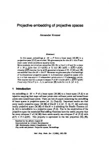
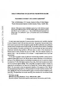
The following proposition is easy to verify explicitly: Proposition 2.0.5. An n-pointed rooted tree of d-dimensional projective spaces is stable if and only if it has no nontrivial automorphisms. As a simple example, consider a stable (n + 1)-pointed rational curve consisting of three components Zi ∼ = P1 such that Z2 and Z3 are attached to Z1 by identifying for each i ∈ {2, 3} a point hi ∈ Xi with ei ∈ X1 . Suppose there are s ≥ 2 points p1 ,. . . , ps ∈ X2 \ {h2 } and n − s ≥ 2 points ps+1 ,. . . pn ∈ X3 \ {h3 } and the (n + 1)-st point pn+1 is on Z3 \ {e2 , e3 }. The curve is a tree of projective lines and is illustrated below in figure 1. We call pn+1 ∈ X1 the root of the tree. More generally, let Z1 = Bl{q,q′ } Pd be the blow up of Pd at the points q and q ′ with exceptional divisors E2 and E3 , and let H1 = Pd−1 ֒→ Z1 \{q, q ′} be an embedded hyperplane. Let Z2 be isomorphic to Pd with fixed marked points p1 ,. . . , ps ∈ Z2 and a fixed embedded hyperplane H2 = Pd−1 ֒→ Z2 \ {p1 , . . . , ps }. Finally, let Z3 be isomorphic to Pd with marked points ps+1 ,. . .,pn ∈ Z3 and an embedded hyperplane H3 = Pd−1 ֒→ Z3 \ {ps+1 , . . . , pn }. Let H2 be identified pointwise with E2 and H3 with E3 . When the components are attached, they from a tree. We call the embedded hyperplane H1 = Pd−1 ⊂ X1 the root of the tree, shown below in figure 2 when d = 2. If s ≥ 2 and n − s ≥ 2, the tree is stable; it has no nontrivial automorphisms fixing the embedded hyperplanes pointwise which preserve the marked points. 6
1 0
00 11 00 11 11 00 00 11
X2
0 1 1 0
{q1,..,q t}
{p1,..,p s} 1 0 0 1
11 00
p
n+1 11 00
e2=h2
0 1 11 00
1 0
X3
1 0
1 0 0 1
E3 H2
H3
E2
00000000000 11111111111 X11111111111 00000000000 2 00000000000 11111111111
e3=h 3
11111111111 00000000000 00000000000 11111111111 00000000000 11111111111 00000000000 11111111111 00000000000 11111111111 00000000000 11111111111 00000000000 11111111111 00000000000 11111111111 1 00000000000 11111111111 00000000000 11111111111 00000000000 11111111111
H
X1
Figure 1. d = 1
1 0
{q 1,..,q t} 0 00 11 00 11 1
{p1 ,..,p s}
X3 X1
Figure 2. d = 2
3. Definition and Inductive Construction of Td,n In this section we define the variety Td,n as an abstract variety. This is done by using the construction of the Fulton-MacPherson configuration space as in [FM94]. 3.1. Inductive Construction of the Fulton-Macpherson Space. Let X be a smooth variety of dimension d, and let x ∈ X(k). As in [FM94], we let X[n] denote the Fulton-MacPherson configuration space of n points on X, whose construction we recall below (with some minor changes in notation). Set N = {1, . . . , n}. The space X[n] comes with a morphism X[n] → X n . For every subset S ⊂ N with |S| ≥ 2, Fulton and MacPherson define a codimension 1 smooth subvariety D(S) ⊂ X[n] which maps into the diagonal ∆S = {(xi ) ∈ X n |xi = xj for i, j ∈ S}. In particular, we have a morphism π : D(N) → X ∼ = ∆N ⊂ X n . X,x Definition 3.1.1. Td,n = π −1 (x).
We shall prove that this definition does not depend on the smooth variety X or on the point x ∈ X(k). Thus we simply write Td,n for X,x Td,n . To show this, we describe the functor which it represents later in this section and show that this functor is independent of our choices (see Definition 3.6.1). We also show that the points of Td,n correspond to the n-pointed stable d-RTPS’s from the previous section (Theorem 3.4.4). In order to set notation and motivate our work on the spaces Td,n , we now recall Fulton and MacPherson’s construction of X[n]. The construction of these spaces is given inductively. It will be notationally convenient to let N = {1, . . . , n}, and we may occasionally write X[N] to mean X[n]. For a subset S ⊂ N we let S + be the subset S ∪ {n + 1} ⊂ {1, . . . , n + 1}. In particular, N + = {1, . . . , n + 1}. At the n’th step in the process, we will have constructed: (1) a space X[n], 7
(2) a morphism πn : X[n] → X n (which we will write as π when n is understood), (3) for each subset S ⊂ N with |S| ≥ 2, a divisor D(S) ⊂ X[n]. We begin by giving the definition of the first two spaces directly. For n = 1, we set X[1] = X. For n = 2, we let X[2] = Bl∆ (X × X) be the blowup of X × X along the diagonal ∆. We define D({1, 2}) to be the exceptional divisor of this blowup, and let π : X[2] → X 2 be the blowup map. To go from X[n] to X[n + 1] requires a series of steps in itself. We’ll construct a sequence of smooth varieties: ρn
ρk+1
ρn−1
X[n, n] −→ X[n, n − 1] −→ · · · −→ X[n, k + 1] −→ X[n, k] −→ ρ1
· · · −→ X[n, 1] −→ X[n, 0], so that X[n, n] = X[n + 1]. We will define these varieties X[n, k] inductively with respect to k. At each step, we will construct for 0 ≤ k ≤ n: (1) a smooth variety X[n, k], (2) a morphism ρk : X[n, k] → X[n, k − 1] when k > 0, (3) smooth subvarieties X[n, k](S ′ ) for each subset S ′ ⊂ N + with at least two elements. In the case k = 0, we set X[n, 0] = X[n] × X. For S ′ ⊂ N ⊂ N + , we define X[n, 0](S ′) = D(S ′ ) × X. Let pi : X[n] → X n → X be the composition of πn with the i’th projection map. We define X[n, 0]({i}+ ) to be the graph of pi - in other words, it is the image of the morphism id × pi : X[n] → X[n] × X. Now suppose that S ⊂ N, |S| ≥ 2. It turns out that if i, j ∈ S, then if we let Γi = id × pi : D(S) −→ D(S) × X, the images Γi (D(S)) and Γj (D(S)) are isomorphic. We denote these common maps by ΓS and define X[n, 0](S + ) to be the image ΓS (D(S)). The variety X[n, 1] is defined to be the blowup of X[n, 0] along the subvariety X[n, 0](N + ). For S ′ 6= N + , the variety X[n, 1](S ′ ) is defined to be the proper transform of X[n, 0](S ′ ), and we define X[n, 1](N + ) to be the exceptional divisor. We have the following pullback diagram: X[n, 1](N + )
P (NN )
X[n, 1] /
ρ1
� � +
X[n, 0](N ) /
X[n, 0]
X[n] × X,
where NN = NX[n,0](N + ) X[n, 0] is the normal bundle of X[n, 0](N + ) in X[n, 0] and X[n, 1](N + ) = P (NN ) is the exceptional divisor of the 8
blowup. It will be useful to consider the first Chern class of this bundle, and so we will set lN = c1 (ONN (1)). Once X[n, k] has been constructed for k ≥ 1 along with its subschemes X[n, k](S ′ ), the variety X[n, k +1], together with its morphism ρk+1 : X[n, k + 1] → X[n, k], is defined to be the blowup along the disjoint union of the subvarieties X[n, k](U + ), where U ranges over all subsets of N of cardinality n − k. Fulton and MacPherson prove that these subvarieties are all disjoint ([FM94]). For S ′ = U + where U ⊂ N, |U| = n − k, we define X[n, k + 1](U + ) to be the exceptional divisor in X[n, k + 1] lying over X[n, k](U + ). For S ′ ∈ N + not of this form, we define X[n, k + 1](S ′ ) to be the proper transform of X[n, k](S ′ ). For each U ⊂ N of cardinality |U| = n − k we have the following pullback diagram: X[n, k + 1](U + )
P (NU ) /
X[n, k + 1]
�
X[n, k](U + )
� /
X[n, k],
where NU = NX[n,k](U + ) X[n, k] is the normal bundle of X[n, k](U + ) in X[n, k] and X[n, k + 1](U + ) = P (NU ) is the exceptional divisor of the blowup. We write lU = c1 (ONU (1)). To complete the construction of X[n + 1] = X[n, n], we define for ′ S ∈ N + , X[n + 1](S) = X[n, n](S ′ ) and π : X[n + 1] → X n to be the composition X[n + 1] = X[n, n]
ρ1 ◦···◦ρn
/
X[n, 0] = X[n] × X
πn ×idX
/
Xn
For convenience of notation, we define X[n, i](S1 , . . . , Sk ) = X[n, i](S1 )∩ · · · ∩ X[n, i](Sk ). Theorem 3.1.2. Let ∅ = 6 S ⊂ N 6= 2, |S| = i. Choose a ∈ N. Then: (1) The morphisms X[n, n−1]({a}+ ) → X[n] and X[n, n−s](S + ) → X[n, 0](S + ) ∼ = D(S) are isomorphisms for |S| ≥ 2. (2) The morphism X[n, 1](N + ) → X[n, 0](N + ) is a projective bundle morphism of relative dimension d. (3) The morphism X[n, i+1](N + ) → X[n, i](N + ) for 1 ≤ i ≤ n−1 is a blowup along the union of subvarieties X[n, i](N + , S + ) for S ⊂ N, |S| = n − i. (4) For S as above, the morphism X[n, i](N + , S + ) → X[n, 0](N + , S + ) is an isomorphism. 9
Proof. Parts 1, 2, and 3 follow from [FM94] proposition 3.5. For part 4, we have by part 1, X[n, i](S + ) → X[n, 0](S + ) is an isomorphism. Consequently, when we restrict to X[n, i](N + , S + ), we get an isomorphism � X[n, i](N + , S + ) ∼ = X[n, 0](N + , S + ). 3.2. Functors of points related to the Fulton-Macpherson space. It will be useful for us to have a description of the functors represented by the varieties X[n, i] and X[n, i](S1 , . . . , Sk ). Suppose H is a variety and h : H → X n+1 is a morphism. For a subset S ⊂ N, we use the notation hS to denote the composition of h with the projection + X N → X S , and we write ha for h{a} . Let ∆S ⊂ X S denote the (small) diagonal, and IS the ideal sheaf of ∆S in X S . Note that for S1 ⊂ S2 , the projection X S2 → X S1 induces a morphism h∗S1 IS1 → h∗S2 IS2 . Definition 3.2.1. Let H and h be as above. A screen for h and S ⊂ N + is an invertible quotient φS : h∗ IS → LS . A collection of screens φS1 , . . . , φSk is compatible if whenever Si ⊂ Sj , there is a unique morphism LSi → LSj which makes the following diagram commute: h∗Si ISi /
�
L Si �
h∗Sj ISj /
L Sj
Definition 3.2.2. A subset S ⊂ N + satisfies property Pi , (S ∈ Pi ) if either S ⊂ N, |S| ≥ 2 or S = T + , |T | > n − i. Definition 3.2.3. We define the functor X [n, i] from the category of schemes to the category of sets by setting X [n, i](H) to be the set of pairs � � + (h : H → X N ), {φT : h∗T IT → LT }T ∈Pi , such that the φT ’s form a compatible collection of screens. We define the subfunctor X [n, i](S1 , . . . , Sk ) by setting X [n, i](S1 , . . . Sk )(H) to be the subset of X [n, i] such that whenever T ∈ Pi with |T ∩ Sj | ≥ 2 and T 6⊂ Sj for some j, the compatibility morphism LT ∩Sj → LT is zero. The following theorem is useful not only for understanding the iterative construction of the space Td,n , but also for the applications to the Fulton-MacPherson configuration space in Section 4. Theorem 3.2.4 ([FM94]). The functors X [n, i] and X [n, i](S1 , . . . , Sk ) are represented by the varieties X[n, i] and X[n, i](S1 , . . . , Sk ) respectively. 10
3.3. Inductive construction of Td,n . We now present an inductive construction of Td,n as a sequence of blowups of a projective bundle over Td,n−1 . This allows us to give an explicit inductive presentation of its Chow groups, its Chow motive and in the next section, a description of its Poincar´e polynomial. i Theorem 3.3.1. There is a sequence of smooth varieties Fd,n , for 0 ≤ i + i ≤ n, with subvarieties Fd,n (T ) indexed by T ( N , |T | ≥ 2 and i+1 i morphisms bi : Fd,n → Fd,n such that: 0 n (1) Fd,n = Td,n and Fd,n = Td,n+1 , 1 0 (2) the morphism b0 : Fd,n → Fd,n = Td,n is a projective bundle morphism of relative dimension d, (3) the morphisms bi for 1 ≤ i ≤ n − 1 are blowups along the union i of the subvarieties Fd,n (S + ), |S| = n − i, i (4) Fd,n (S + ) ∼ = Td,s × Td,n−s+1 where s = |S| = n − i if i 6= n − 1, n−1 (5) Fd,n ({a}+ ) ∼ = Td,n .
This theorem closely parallels the above situation for the Fulton MacPherson configuration space X[n + 1] from X[n] × X, and in fact we derive it mainly as a consequence of a careful analysis of certain aspects of this construction. Although very similar in structure to the construction of Keel [Kee92] in the case d = 1, we note that our construction is different. For example, the analog of our (nontrivial) projective bundle b0 in Keel’s construction is always a trivial vector bundle. i The varieties Fd,n and Fd,n (S) are defined as follows: Definition 3.3.2. Let X be a smooth projective d-dimensional variety, and choose x ∈ X(k). We abuse notation slightly (by using the symbol π in two different ways) and let π : X[n, i](N + ) → X be the composition X[n, i](N + ) /
X[n, i]
ρ1 ···ρi
/
X[n] × X
π×idX
/
X n+1 /
where the final arrow is any of the projections (all give the same rei i sult). We define Fd,n to be π −1 (x) = X[n, i](N + ) ×X x and Fd,n (S) = + + 0 + 0 X[n, i](N , S )×X x. We also define Td,n (S) = Fd,n (S ) ⊂ Fd,n = Td,n . The proof of Theorem 3.3.1 follows from the following proposition combined with Theorem 3.1.2. Proposition 3.3.3. Suppose X is a smooth variety with trivial tangent bundle, and let S ⊂ N, |S| = s. Then if 0 ≤ i ≤ s, we have an i isomorphism X[n, n − s + i](S + ) = X[n − s + 1] × Fd,s commuting with the natural projections to X[n − s + 1]. 11
X
In particular, in proving this proposition, it immediately follows that Definitions 3.3.2 and 3.1.1 do not depend on the variety X or on the point x, since the tangent bundle is locally trivial. Note that it follows that for X with trivial tangent bundle, we have X[n, n−s+i](S + , T + ) ∼ = i X[n−s+1]×Fd,n (T + ) for T ( S by restricting the above isomorphism. Remark 3.3.4. We see by this reasoning that in definition 3.3.2, the maps π : X[n, i](N + ) → X and π|X[n,i](N + ,S + ) locally have a product structure as above, and so in particular, [Fd,n (S)] = ι!x [X[n, i](N + , S + )] in the Chow groups of X[n, i](N + ) and Fd,n respectively, where ιx is� � the inclusion of the point x into X. Since the class X[n, i](N + , S + )� � on X[n, i](N + ) can also be seen as the Gysin pullback j ! X[n, i](S + ) where j : X[n, i](N + ) �֒→ X[n, i] is � the natural embedding, we may + ! ! + write [Fd,n (S )] = ι j X[n, i](S ) , and it makes �sense therefore � to abuse notation and formally define [Fd,n (N + )] = ι! j ! X[n, i](N + ) . We 0 also set [Td,n (S)] = [Fd,n (S + )]. proof of proposition 3.3.3. By Theorem 3.2.4, we may translate a morphism to X[n, n − s + i](S + ) to a collection of screen data. Suppose f : H → X[n, n − s + i](S + ) corresponds to a collection of screens � � + (h : H → X N ), {φT : h∗T IT → LT }T ∈Pi .
Note that if T ⊂ S or T = S + , the function hT maps entirely into the diagonal ∆T ⊂ X T , and so by factoring hT through ∆T ∼ = X, we may ∗ identify hT IT� with the pullback of the conormal sheaf h{a} IT /IT2 = ∗ (T X)T /T X , where a ∈ T . Note that we have h{a} = h{b} for any b ∈ S + , and so it suffices to choose a ∈ S + . The screen for T therefore translates to specifying a 1-dimensional sub-vector bundle iT : LT ֒→ (T X)T /T X compatible with respect to the natural projec′ tions (T X)T /T X → (T X)T /T X for T ′ ⊂ T . Since V is trivial, we may write T X = VX where V is a vector space over k of dimension d. Let Fd,s (H) denote the set of collections of compatible line sub-vector bundles of the form {iT : LT ֒→ V T /V }T ⊂S or T =S + . It is not hard to check from this description that Fd,s in fact defines a functor which is represented by Fd,s . To complete the proof, we note that by the above, a morphism to i X[n, n − s + i](S + ) gives a morphism to Fd,s . We may also obtain a morphism to X[n − s + 1] by choosing a point a ∈ S + and keeping only the screens for subsets T ⊂ (N \ S) ∪ {a}. This gives a morphism X[n, n − s + i](S + ) → X[n − s + 1] × Fd,s . We may obtain an inverse morphism by describing how to take the screens for T ⊂ (N \ S) ∪ {a} together with the screens for T ⊂ S + and define screens for the 12
remaining T ∈ Pn−s+1 . This is done in a way similar to the proof of Theorem 3.1.2, part 1 and we leave the detailed proof to the reader. We mention as a guide that for T of the form T = U ∪R where U ⊂ S + and R ∩ S + = ∅, we set LT = LR∪{a} if R 6= ∅, and otherwise LT = L∗T if T ⊂ S + . � proof of Theorem 3.3.1. Note that we may obtain the product decomposition Td,n (S) ∼ = Td,s × Td,n−s+1 , where s = |S| by letting X be a variety with trivial tangent bundle and considering the commutative diagram where the upper square is a pullback: X[n, n − s + i](S + , N + ) i fibers ∼ = Fd,s
/
X[n, n − s + i](S + ) i fibers ∼ = Fd,s
�
� �+ � X[n − s + i, 0] (N \ S) ∪ {a}
� /
X[n − s + 1]
fibers ∼ = Td,n−s+1
�
�
X
X �
3.4. Basic properties of Td,n . We now give an example of these spaces for “minimal” values of n: Proposition 3.4.1. We have isomorphisms T1,3 ∼ = P1 and for d > 1, d−1 Td,2 ∼ = P . Under these identifications, [T1,3 ({1, 2, 3})] = OP1 (−1), and [Td,2 ({1, 2})] = OPd−1 (−1). Proof. First consider the case of Td,2 . We know that Ad [2] = Bl∆ (Ad × Ad ), and that D({1, 2}) is the exceptional divisor of the blowup [FM94]. Therefore D({1, 2}) = P (N∆ (Ad × Ad )) ∼ = Pd−1 × Ad . In particular, Td,2 ∼ = Pd−1 as claimed. For the case of T1,3 , we note that A1 [3] = Bl∆ (A1 )3 , where ∆ is the small diagonal with exceptional divisor D({1, 2, 3}). � Corollary 3.4.2. Td,n is a smooth projective rational variety of dimension dn − d − 1. Proof. This follows from induction on n, with base case proven in Proposition 3.4.1 and inductive step given by Theorem 3.3.1. � Proposition 3.4.3. T1,n ∼ = M 0,n+1 . 13
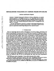
Proof. Since each n pointed stable 1-RTPS is exactly an (n+1)-pointed stable curve (where the root hyperplane is identified with the (n + 1)st + marking), the family Td,n → Td,n gives a morphism Td,n → M 0,n which is bijective on k points. To show this is an isomorphism, it suffices to construct an inverse morphism. To do this, consider the Fulton-MacPherson configuration space P1 [n], and the divisor D(N) on P1 [n]. By Definition 3.1.1, we may identify T1,n with a fiber of the natural morphism D(N) → P1 . By [MM] (pages 4,5), there is a natural isomorphism M 0,n (P1 , 1) ∼ = P1 [n]. Note that by [FP] (Theorem 2, part 3), M 0,n (P1 , 1) is actually a fine moduli space for stable maps of degree 1 to P1 . The isomorphism from [MM] identifies the divisor D(N) with the stable maps f : (C, p1, . . . , pn ) → P1 which take all the marked points to a given point x ∈ P1 . The natural morphism D(N) → P1 is simply the morphism taking this stable map to x. For such a stable map, the semistable curve C must have the form: D1 D2
D4
1 0 1 0 11 00
1 0 1 0
1 0 1 0
D3
11 00
1 0 0 1
C’
q
Since M 0,n (P1 , 1) is a fine moduli space, one may check that the fiber over a given point x ∈ P1 is also a fine moduli space for (n + 1)pointed stable curves. To see this, suppose we have a stable map f : (C, p1, . . . , pn ) → P1 in this fiber, where the semistable curve C has irreducible components C ′ , D1 , . . . , Dr , with f∗ ([C ′ ]) = 1, f∗ ([Di ]) = 0. Since none of the marked points pi may lie on C ′ , the curve remaining after forgetting C ′ , composed of the union of the Di , is a (n+1)-pointed stable rational curve where the (n + 1)st marking is obtained from the point where ∪Di intersects C ′ . This gives an isomorphism of the fiber over x with M 0,n+1 which is inverse to the morphism above. � Theorem 3.4.4. The points of Td,n are in one to one correspondence with isomorphism classes of n-pointed stable rooted trees of d-dimensional projective spaces. Proof. Let X[n]+ → X[n] be the “universal family” as described in [FM94]. By base change over Td,n → X[n] (included by choosing a + point x ∈ X), we obtain a flat family Td,n → Td,n . It follows from the description in [FM94] that the fibers are all n pointed stable d-RTPS’s, exactly one in each isomorphism class. � 14
3.5. Ample divisor classes on Td,n . Although by 3.4.2, we know abstractly that Td,n is a projective variety, it is often useful to have an explicit presentation of an ample divisor. We exhibit such a divisor below: Theorem 3.5.1. Let δS = [Td,n (S)] in the Chow group of Td,n as in remark 3.3.4. Then for S ⊂ N, |S| ≥ 2, the divisor classes X ηS = δT N ⊇T ⊇S
is nef and base point free. Furthermore, any expression of the form X A= cS ηS S⊂N,|S|≥2
is very ample provided cS > 0 for all S.
Proof. By [FM94], we have for any smooth d-dimensional variety X, an embedding Y i : X[n] ֒→ Bl∆S (X S ), S⊂N,|S|≥2
S
where ∆S ⊂ X is the (small) diagonal. Let iS be the morphism i composed with the projection map onto the factor Bl∆S (X S ). If AS is an very ample class on Bl∆S (X S ), then it follows immediately that i∗S (AS ) is nef and base free (since it is the pullback of a very ample P point divisor), and that cS i∗S (AS ) is very ample on X[n] if each cS > 0 (since it is the pullback of a very ample divisor via an embedding). Let BS′ be a very ample divisor class on X S , and let IS be the ideal sheaf of ∆S in OX S . Let fS : Bl∆S (X S ) → X S be the natural projection. Then fS−1 (IS ) is an invertible sheaf and the divisor class λfS∗ BS + c1 (f −1 (IS )) is very ample for some λ > 0 (see [Har77], Proposition 7.10(b) and the proof of 7.13(a)). Let BS = λBS′ . Then � �� αS = i∗S fS∗ BS + c1 f −1 (IS ) is nef and base point free. Fix for the remainder of the proof integers cS > 0. Then � X �� α= i∗S fS∗ BS + c1 f −1 (IS ) S⊂N,|S|≥2
is very ample on X[n].
j
Now consider the embedding Td,n ֒→ X[n], and let jS be the composition with the projection to Bl∆S (X S ). Let ηS = j ∗ αS , and A = j ∗ α. Since j is an embedding, ηS is nef and base point free and A is very 15
ample. We will be done once we show that the divisors ηS have the desired form. To begin, we may rewrite ηS in the following way: � ηS = j ∗ αS = fS∗ BS + c1 fS−1 (IS ) � = j ∗ i∗S fS∗ BS + j ∗ c1 i∗S fS−1 (IS ) � = (fS ◦ iS ◦ j)∗ BS − j ∗ c1 i∗S fS−1 (IS ) Examining the second term, we see by lemma 7.2.1, that i∗S fS−1 (IS ) = (fS ◦ iS )−1 (IS ), and by [FM94], page 203, if we let I(D(S)) be the Q −1 ideal sheaf of D(S) ⊂ X[n], we have (fS ◦ iS ) (IS ) = T ⊃S I(D(T )). Consequently, taking first Chern classes and applying j ∗ , we have: X X X � j ∗ c1 i∗S fS−1 (IS ) = j ∗ c1 (I(D(T ))) = j ∗ −[D(T )] = − δT . T ⊃S
T ⊃S
T ⊃S
On the other hand, looking at the first term, (fS ◦ iS ◦ j)∗ BS , we see that since the morphism (fS ◦ iS ◦ j) factors through a morphism to Spec(k), whose Picard group is the zero group, this pullback must in fact vanish. Therefore we have X ηS = δT , S⊂T ⊂N
as desired.
�
3.6. A relative version of Td,n . It will be useful in what follows to have a relative version of construction of Td,n . This follows without much technical difficulty and we leave some of the routine verifications to the reader. Definition 3.6.1. Let V be a rank d vector bundle over a scheme X. We define the functor TV,n from the category (Sch/X)op of X-schemes to the category of sets as follows. For h : H → X, we define TX,n (H) to be the set of collections {φT : h∗ V → LT }T ∈N,|T |≥2, such that the φT ’s form a compatible collection of screens (in the same sense as in 3.2.1). Note that there is a canonical morphism (natural transformation) from TV,n to X. By setting TV,1 = X, TV,2 = P rojX (Sym•V ), we may inductively dei fine varieties TV,n , FV,n , FV,n (S + ) such that the following theorem holds: i Theorem 3.6.2. There is a sequence of schemes FV,n , for 0 ≤ i ≤ n, i + with subschemes FV,n (T ) indexed by T ( N , |T | ≥ 2 and morphisms i+1 i bi : FV,n → FV,n such that:
16
0 n (1) FV,n = TV,n and FV,n = TV,n+1 , 1 0 (2) the morphism b0 : FV,n → FV,n = TV,n is a projective bundle morphism of relative dimension d, (3) the morphisms bi for 1 ≤ i ≤ n − 1 are blowups along the union i i of the subschemes FV,n (S + ), and FV,n (S + ) ∼ = TV,s ×X TV,n−s+1 n−1 + ∼ if i 6= n − 1 and FV,n ({a} ) = TV,n , (4) TV,n is represented by TV,n .
The proof of this theorem takes the following steps. First, we see that it holds in the case that V is a trivial bundle by noting that the inductive construction of the space Td,n+1 from Td,n by taking a projective bundle and blowing up may be fibered with a scheme X to give an inductive construction of Td,n+1 × X = TV,n+1 from Td,n × X = i TV,n . For a general bundle, we may define the functors FV,n (S + ) by + + emulating the definition of X [n, i](N , S ), and note that they are locally represented subschemes over subsets where V is trivial, and i that these subschemes glue to give a closed subscheme FV,n (S + ). We i+1 i define FV,n to be the blowup along the subschemes FV,n (S + ) where |S| = i. Since these have the correct functorial description locally, we i+1 i+1 may glue and conclude that FV,n represents the functor FV,n . We note the following lemmas which will be useful in Section 4: Lemma 3.6.3. Let V be a vector bundle on X, and let π : TV,n → X be the natural projection. Then TV,n ×X TV,m = Tπ∗ TV,n ,m . Lemma 3.6.4. Let X be any scheme, and let V be a trivial vector bundle of rank d on X. Then Td,n × X ∼ = TV,n . In particular, if X = Spec(k) then TV,n ∼ = Td,n . Lemma 3.6.5. Let X be a smooth variety and let D(S) ⊂ X[n] be the divisor on the Fulton-MacPherson configuration space described in the beginning of the section. If π : D(S) → X[n − |S| + 1] = X[(N \ S) ∪ {a}] is the natural morphism from projecting with respect to the subset (N \ S) ∪{a} where a ∈ S, and f : X[(N \ S) ∪{a}] → X the projection with respect to a, then there is a natural isomorphism D(S) = Tf ∗ ΩX ,s . The proofs of these are elementary and follow from an examination of the functorial descriptions of the spaces involved. Remark 3.6.6. The morphism Td,n+1 → Td,n obtained by composing the morphisms bi of theorem 3.6.2 is given functorially by dropping all screens for subsets S ⊂ N + which contain the (n + 1)st marking. In the future, we denote this morphism by πn+1 . We may similarly define morphism πi for any i ∈ N + by dropping the ith marking. 17
4. Inductive presentations of Chow groups and motives We consider the Chow group of a variety X as a graded abelian group A(X) = A∗ (X). We use the following general conventions. For a graded abelian group M = ⊕i∈Z Mi , we set M(n) to be the group with grading shifted so that (M(n))i = Mn−i . The grading on the tensor product M ⊗ N = M ⊗Z N is given by (M ⊗ N)n = ⊕i+j=n Mi ⊗ Nj . We write Z for the graded abelian group with the integers in degree 0 and zero in all other degrees. Remark 4.0.7. All the constructions used in this section are motivic: in other words, if the reader prefers, they may interpret A(X) as M(X), the Chow motive of X (as in [Man68]), M(i) to be M twisted i times with the Lefschetz motive, and Z to be the motive of Spec(k). In this notation we have the following well known facts: Lemma 4.0.8. For V a vector bundle of rank d on X, A(P (V )) =
d−1 M
A(X)(i) = A(X) ⊗ (
i=0
d−1 M
Z(i)) = A(X) ⊗ A(Pd−1 ).
i=0
Proof. [Ful98] for Chow groups, [Man68] for Chow motives.
�
Lemma 4.0.9. For Z ֒→ X a regularly embedded subvariety of codimension d, A(BlZ X) = A(X) ⊕
d−1 M i=1
� � A(Z)(i) = A(X) ⊕ A(Z) ⊗ A(Pd−2 (1)) .
Proof. [Man68]
�
One technical difficulty which makes the computation of Chow groups more difficult than the computation of cohomology is the fact that the Chow group of a product X × Y is not easily expressible in terms of the Chow groups of X and Y . Philosophically, we show in this section that products (and certain fiber bundles) with Td,n as one of the factors are not subject to this difficulty. 4.1. The Chow groups and motives of Td,n . 18
Theorem 4.1.1. Let V /X be a vector bundle of rank d. Then ! d M A(TV,n+1 ) = A(TV,n )(j) ⊕ d M
j=0
M
j=1 S(N,|S|≥2
A(TV,|S| × TV,n−|S|+1)(j) ⊕
d−1 M M
A(TV,n )(j)
j=1 a∈N
!
Proof. This is an immediate consequence of Theorem 3.6.2 together with Lemmas 4.0.8 and 4.0.9. � Using Lemma 3.6.4 to identify Td,n × B = TOBd ,n for a variety B, we obtain the following corollary: Corollary 4.1.2. Let V /X be a vector bundle of rank d. Then ! d M A(Td,n+1 × B) = A(Td,n × B)(j) ⊕ d M
j=0
M
j=1 S(N,|S|≥2
A(Td,|S| × Td,n−|S|+1 × B)(j)⊕
d−1 M M
A(Td,n × B)(j)
j=1 a∈N
In particular, setting B = Spec(k), we obtain a presentation for the Chow groups of Td,n+1 in terms of the Chow rings of varieties of the form Td,t × B for various values of t < n. These terms may be successively reduced using corollary 4.1.2, eventually using the fact that A(T1,3 ) = A(P1 ) = Z ⊕ Z(1) or the fact A(Td,2 ) ∼ = A(Pd−1 ) = ⊕d−1 i=0 Z(i) from Lemma 3.4.1. 4.2. The Chow groups and motives of the Fulton-MacPherson configuration space. Fulton and MacPherson have given a compactification X[n] of the moduli space of n distinct points on a smooth variety X as well as a presentation of the intersection ring of the space X[n]. They pose the following problem ([FM/Ann94], page 189): ”It would be interesting to find an explicit basis for the Chow groups of Pm [n], preferably simple with respect to the intersection pairings, as Keel has done in the case m = 1.” In this section, we present an inductive presentation of the Chow groups and motives of the spaces X[n] which parallels Keel’s presentation in [Kee92]. 19
!
Let us begin by making an elementary observation. The blowup construction of the Fulton-MacPherson space described in Section 3 gives X[n + 1] as a composition of blowups of X[n] × X. In the same way, we easily obtain X[n+1]×B as a composition of blowups of X[n]× X ×B for an arbitrary variety B. Together with the identifications from Theorem 3.1.2, part 1, this yields the following inductive presentation: Theorem 4.2.1. Let X be a smooth variety. Then A(X[n + 1] × B) = A(X[n] × X × B)⊕ ! d d−1 M M M M A(D(S) × B)(j) ⊕ A(X[n] × B)(j) j=1 S(N,|S|≥2
j=1 a∈N
As before, the symbol A can stand either for the Chow group or the Chow motive. In particular, setting B = Spec(k), we obtain a presentation for the Chow groups (or motives) of X[n + 1] in terms of the Chow groups (or motives) of the varieties D(S) and X[n] × X. From Lemma 3.6.5, we have an isomorphism D(S) = TV,s , for a vector bundle V of rank d on X[n − s + 1]. These terms may be successively reduced using theorems 4.1.1 and 4.2.1, eventually yielding an answer in terms only of the Chow groups of X T for T = 1, . . . , n. In general there is no known formula for the Chow groups of X T in terms of the Chow groups of X, however, if X has a cellular decomposition (see definition 7.3.2), then it is true that A(X T ) = ⊗a∈T A(X). 5. Betti numbers and Poincar´ e polynomials In this section, we analyze generating functions for the Betti numbers and Poincar´e polynomials of the varieties Td,n in the case when k = C. By Corollary 7.3.4, the Betti numbers coincide with the ranks of the Chow groups, and therefore, since the presentation of the Chow groups of Td,n is independent of the underlying field k, these determine the Chow groups in general. A recursive description of these polynomials was given in [FM94] for the spaces X[n]. In [Man95], Manin relates the Poincar´e polynomials of these spaces as well as the polynomials for M 0,n to solutions to certain differential and functional equations. We apply Manin’s ideas here to obtain similar results for Td,n , which specialize to Manin’s original result for M 0,n+1 in the case d = 1. Indeed, the defining equations for the generating functions of Td,n described here are identical to those discussed by Manin (Theorem 0.4.1) in his analysis of the Poincar´e polynomials of X[n]. In our case, we recover these equations from the explicit blowup construction of 20
Td,n , just as one can recover Theorem 0.3.1 of Manin from the blowup construction of M 0,n of Keel. For a smooth compact variety Z, denote its Poincar´e polynomial by P PZ (q) = j dim H j (Z)q j . In particular, put κm = PPm−1 (q) =
q 2m − 1 . q2 − 1
Fix d, and for n ≥ 2, denote by Pn (q) = PTd,n (q) the Poincar´e polynomial of Td,n . From corollary 7.3.4 and the inductive presentation of the Chow groups of Td,n in section 4.1, we have the following recursion for the Poincar´e polynomials Pn (q). X � n (1) Pn+1 (q) = (κd+1 + nq 2 κd−1 )Pn (q) + q 2 κd Pi (q)Pj (q) i i+j=n+1 2≤i≤n−1
Pn (q) , this is equivalent Defining P1 (q) = 1, and defining pn = pn (q) = n! to either of the recursions: X (n + 1)pn+1 = (κd+1 + nq 2 κd−1 )pn + q 2 κd jpi pj (n+1)pn+1 = (κd+1 +nq 2 κd−1 )pn +q 2 κd
X
i+j=n+1 2≤i≤n−1
jpi pj −q 2 κd npn −q 2 κd pn .
i+j=n+1 i≥1
The fact that κd+1 = 1 + q 2 κd , q 2 κd−1 = κd − 1, and that q 2 κd = q − 1 + κd shows that the recursion in (1) can be rewritten as: X (2) (n + 1)pn+1 (q) = (1 − nq 2d )pn (q) + q 2 κd jpi (q)pj (q). 2d
i+j=n+1 i≥1
Consider the following generating function, recalling that p1 (q) = 1: X X ψ(q, t) = t + pn (q)tn = pn (q)tn . n≥2
n≥1
Theorem 5.0.2. ψ(q, t) is the unique root in t + t2 Q[q][[t]] of the following functional equation in t with parameter q: (3)
κd (1 + ψ)q
2d
= q 2d+2 κd ψ − q 2d (q 2d − 1)t + κd
or the following differential equation in t with parameter q: (4)
(1 + q 2d t − q 2 κd ψ)ψt = 1 + ψ.
Proof. First, note that we get (4) from (3) by differentiating in t. Moreover, we can see that the equations are equivalent to the recursion (1) 21
P or (2). In particular, since ψt (q, t) = n≥1 npn (q)tn−1 , the tn term for n ≥ 1 of the left hand side of the differential equation is X (n + 1)pn+1 + q 2d npn − q 2 κd jpj pi i+j=n+1 i≥1,j≥1
which is equal to pn by (2), and for n = 0 is p1 = 1. This is exactly the statement of the theorem. � P Fix d ≥ 1 and define the generating function η(t) = t+ n≥2 χ(Td,n ). Corollary 5.0.3. η(t) is the unique root in t + t2 Q[q][[t]] of any of the following equations: d(1 + η) log(1 + η) = (d + 1)η − t (1 + t − dη)ηt = 1 + η. Proof. Differentiating the first equation gives the second. The result follows since the Euler characteristic of a smooth compact variety Z can be defined by χ(Z) = Pz (−1) so that η(t) = ψ(−1, t). � 6. Chow Ring of Td,n and pairing between divisors and curves In this section we examine the structure of the Chow ring of the space Td,n . Let k be an arbitrary field. We recall the definition of the divisors Td,n (S) described in Section 3. Fix d ≥ 1, n ≥ 2, and let δS = [Td,n (S)] be the corresponding cycle class in the Chow group A∗ (Td,n ). We obtain an explicit description of the Chow ring of Td,n by considering the Fulton-MacPherson configuration space Ad [n]. Let i : D(N) ֒→ Ad [n] be the inclusion of the divisor on Ad [N] where all the points coincide, and consider the morphism π : D(N) → Ad . By Definition 3.1.1, Td,n = π −1 (0). Recall that by Proposition 3.3.3, Td,n × Ad ∼ = D(N). This implies that we may regard D(N) as a (trivial) vector bundle over Td,n , and therefore we have a morphism π : D(N) → Td,n , and a flat pullback inducing an isomorphism (π ∗ )−1 : A∗ D(N) ∼ = A∗ Td,n . In particular, one may check from the definitions that if we let D(S) be the divisor defined in [FM94] which we used in Section 3 then for S 6= N, δS = (π ∗ )−1 i! [D(S)]. ! We may similarly define δN = (π ∗ )−1 iX [D(N)]. For any two distinct elements a and b ∈ N, define Σab := δ{ab}∪S . S⊂N \{ab}
22
Theorem 6.0.4. A∗ (Td,n ) ∼ = Z[{δS }S⊂N,2≤|S|≤n]/Id,n , where Id,n is the ideal generated by: (1) δS · δT = 0 for all S, T ⊂ N, such that 2 ≤ |S|, |T | and ∅ = 6 S ∩ T ( S, T ; (2) (Σij )d = 0, for all i,j ∈ N. Proof. This follows from immediately from [FM94], and the isomorphism A∗ (Td,n ) ∼ � = A∗ (D(N)) above. In the remainder of this section, we state and prove the following pairing between 1-cycles and the boundary divisors. Theorem 6.0.5. For T ( N, |T | ≥ 2, define 1-cycles CT ∈ A1 (Td,n ) by d(|T |−1)−1 d(n−|T |)−1 CT := δT · δN . If S ( N, |S| ≥ 2, then d(n−1) if S=T; (−1) n−2 δS · CT = (−1) if d = 1, |S| = 2, S ( T ; 0 otherwise.
Corollary 6.0.6. For d > 1, the 1-cycles CT , |T | ≥ 2 form a Z-basis for A1 (Td,n ). In the case d = 1, the 1-cycles CT , |T | ≥ 3 form a Z-basis for A1 (T1,n ) = A1 (M 0,n+1 ).
Proof. First note that the set {δT }T ⊂N,|T |≥3 forms a Z-basis for the codimension 1-cycles on T1,n , and that the set {δT }T ⊂N,|T |≥2 forms a Z-basis for the codimension 1-cycles on Td,n . Note that the ring described in the theorem does not depend on the choice of the base field. The statement which we have to prove is independent of the choice of k, and we may assume without loss of generality that k = C. By Appendix 7.3.4, the space Td,n is an HI space. Since it is a compact smooth manifold with torsion free cohomology groups, we obtain Poincar´e duality induced by the intersection pairing of divisors and curves. Therefore the CT ’s form a dual integer basis to the DT ’s, up to sign. � In order to prove Theorem 6.0.5, we first establish several identities. For convenience, we denote by δi the divisor class δ{1,2,...,i} . The following is an immediate consequence of Theorem 6.0.4. Lemma 6.0.7. For S, T ⊂ N, i ∈ S, T , and l ∈ T \ S, we have δT · δS = 0 unless S ⊂ T . In particular, if l ∈ T , then δT · δl−1 = 0 unless {1, . . . , l} ⊂ T . 23
d(n−|S|)
Lemma 6.0.8. For S ( N, |S| ≥ 2, δS · δN d(n−j)−1 S 6= N, |S| > j, then δS · δN = 0.
= 0. Consequently, if
Proof. We proceed by induction on n − |S|. The base case n − |S| = 0 holds trivially. Suppose that the result holds for n − |S| < k. Let S ⊂ N, |S| = n − k. Choose i ∈ S and j 6∈ S. By Theorem 6.0.4, if j ∈ T and i ∈ S ∩ T , then δT δS = 0 unless S ( T . Moreover, for such d(n−|S|−1) T 6= N, δT δN = 0 by the inductive hypothesis. Therefore d(n−|S|−1)
0 = (Σi,j∈T δT )d δS δN
d(n−|S|−1)
d = δN δS δN
d(n−|S|)
= δS δN
since (Σij )d = 0 by Theorem 6.0.4.
�
Lemma 6.0.9. Given 2 ≤ j ≤ n, if 1 ≤ k < i ≤ j, T ⊂ {1, . . . i}, |T | = i − k, then d(n−j)−1
d δT · δikd+1 · δi+1 · · · δjd · δN
= 0.
Proof. Renumbering the elements of T , it suffices to take δT = δi−k . We proceed by induction on k. For the base case k = 1, we proceed by induction on j − i with base case i = j. By Lemma 6.0.7, if 1, j ∈ T , then δT δj−1 = 0 unless {1, . . . , j} ⊂ T . Also note that by Lemma 6.0.8, d(n−j)−1 if T 6= N and |T | > j, then δT δN = 0. The relation (Σ1j )d = 0 of Theorem 6.0.4 gives d(n−j)−1
0 = (Σ1,j∈T δT )d · δj−1 · δj · δN
d(n−j)−1
= (δj + δN )d · δj−1 · δj · δN
.
The summands coming from the terms of the binomial expansion of (δj +δN )d with positive degree in δN vanish by Lemma 6.0.8 for δS = δj , giving the result. Now suppose that the result holds for integers less than j − i, If 1, i ∈ T , then δT δi−1 = 0 unless {1, . . . , i} ⊂ T by Lemma 6.0.7. Indeed, δT δi−1 δi · · · δj = 0 unless T = δi , . . . , δj or {1, . . . , j} ( T . The relation (Σ1i )d = 0 of Theorem 6.0.4 gives d(n−j)−1
d 0 = (Σ1,i∈T δT )d · δi−1 · δi · δi+1 · · · δjd · δN
We see that terms involving |T | > j vanish by Lemma 6.0.8. Since terms involving δT = δi+1 , . . . , δj vanish by the inductive hypothesis, we have established the base case k = 1. Suppose that the result holds for integers less than k, and consider the following identity: (k−1)d+1
0 = (Σ1,i−k+1∈T δT )d · δi−k · δi
d(n−j)−1
d · · · δjd · δN · δi+1
By Lemma 6.0.7, δT δi . . . δj = 0 unless {1, . . . , i − k + 1} ⊂ T ⊂ {1, . . . , i}, {1, . . . , j} ⊂ T , or δT = δi , . . . , δj . Terms involving δT , 24
of the first type vanish by the inductive hypothesis, and terms involving |T | > j are zero by Lemma 6.0.8. Therefore, nonzero terms can involve only δT = δi , . . . , δj . Finally, the terms with contributions from δi+1 , . . . , δj vanish by the base case k = 1. Hence we are left with (k−1)d+1
0 = δid δi−k · δi
d(n−j)−1
d · δi+1 · · · δjd · δN
,
proving the proposition.
� d(n−j)−1
Lemma 6.0.10. For j ≥ 1, δ2d · · · δjd · δN
d(n−1)−1
= (−1)j−1 δN
.
Proof. We prove the result by induction on j. The result holds trivially for j = 1. For the base case j = 2, it follows from Lemma 6.0.8 that d(n−2)−1
0 = (Σ1,2∈T δT )d · δN
d(n−2)−1
= δ2d · δN
d(n−2)−1
d + δN δN
.
Suppose that the result holds for integers less than j, and consider d(n−j)−1
d 0 = (Σ1,j∈T δT )d · δ2d · · · δj−1 · δN
.
If 1, j ∈ T , then δT δj−1 = 0 unless {1, . . . , j} ⊂ T by Lemma 6.0.7. Nonzero terms in the expansion can only involve δT = δj , δN by Lemma 6.0.8; moreover, terms involving both δj and δN vanish. Therefore d(n−j)−1
δ2d · · · δjd · δN
d(n−(j−1))−1
d = −δ2d · · · δj−1 · δN
n−2 = −(−1)j−2 δN
as needed, where the final equality holds by the inductive hypothesis. � Proposition 6.0.11. For 1 ≤ j ≤ n, if 1 ≤ i ≤ j and 1 ≤ k ≤ j − i, then d(n−j)−1
dk d δ2d · · · δid · δi+k · δi+k+1 · · · δjd · δN
d(n−1)−1
= (−1)j−k δN
.
Proof. We prove the result by induction on j−i. The base case j−i = 1 so that k = 1 is Lemma 6.0.10. Suppose that the statement holds for integers less than j − i. Consider the identity: d(k−1)
0 = (Σ1,i+1∈T δT )d · δi · δi+k
d(n−j)−1
d · δi+k+1 · · · δjd · δN
Lemma 6.0.7 implies that nonzero contributions involve only δT with {1, . . . , i + 1} ⊂ T . Terms involving δT with |T | > j vanish by Lemma 6.0.8, those involving δT with i + 1 < T | < i + k vanish by Lemma 6.0.9, as do those involving δi+k+1 , . . . , δj . Terms involving both δi+1 and δi+k vanish by Lemma 6.0.9. Hence d(k−1)
d(n−j)−1
d d · · · δj ·δ(i+1)+(k−1) ·δi+k+1 0 = δi ·δi+1
25
d(k)
d(n−j)−1
d +δi ·δi+k ·δi+k+1 · · · δjd δN
.
d Multiplying by δ2d · · · δi−1 δid−1 and applying the inductive hypothesis gives the result: d(k)
d(n−j)−1
d δ2d · · · δid · δi+k · δi+k+1 · · · δjd · δN d(k−1)
d(n−j)−1
d d = −δ2d · · · δi+1 ·δ(i+1)+(k−1) ·δi+k+1 · · · δjd ·δN
d(n−1)−1
= −(−1)j−(k−1) δN
� Proposition 6.0.12.
d(n−1)−1 δN
d(n−1)−1
= (−1)
.
Before proving this proposition, we give a proof of Theorem 6.0.5. Proof of Theorem 6.0.5. Let T ( N with |T | ≥ 2. Without loss of generality, say T = {1, . . . , j}. Then δT · CT is equal to d(j−1)
δj
d(n−j)−1
· δN
d(n−1)−1
= −δN
= (−1)d(n−1)
by Proposition 6.0.11 for i = 1, k = j − 1 and Proposition 6.0.12. Let S ( N. If ∅ = 6 S ∩ T ( S, T , then δS · CT = 0 by Theorem 6.0.4. If S ∩ T = ∅, s ∈ S, then d(n−j−1)−1
0 = (Σ1,s∈T ′ δT ′ )d · δS · δj · δN
d(n−j)−1
= δS · δj · δN
since nonzero summands only involve δT ′ with T ∪ {s} ⊂ T ′ by Lemma 6.0.7, and all these contribute zero unless T ′ = N by Lemma 6.0.8. Therefore δS · CT = 0. If T ( S, then δS · CT = 0 by Lemma 6.0.8. Suppose S ( T . We may assume that S = {1, . . . , j − k} with k ≥ 1. Then d(j−1)−1 d(n−j)−1 δS · CT = δj−k · δj · δN . It follows from Lemma 6.0.9 that this is zero when d(j −1)−1 ≥ dk +1, or equivalently when d(j − k − 1) ≥ 2. We conclude that δS · CT = 0 if d = 1 and |S| ≥ 3, or if d ≥ 2. If d = 1 and |S| = 2, then (n−j)−1
δS · CT = δ2 δjj−2 δN
n−2 = δN = (−1)n−2 .
by Proposition 6.0.11 for i = 2, k = j − 2 and Proposition 6.0.12.
�
It remains to prove Proposition 6.0.12. Since the proof involves spaces Td,n for varying n, for the remainder of this section, we use the more precise notation δS,n = [Td,n (S)]. In this language, we need to show Z d(n−1)−1 δN,n = (−1)d(n−1)−1 . Td,n
We first establish the following lemmas. Lemma 6.0.13. Z Z [T1,3 ({1, 2, 3})] = −1 and T1,3
26
[Td,2 ({1, 2})]d−1 = (−1)d−1 . Td,2
.
Proof. From Lemma 3.4.1, we know that Td,2 ∼ = Pd−1 . As discussed in the beginning of the section, [Td,2 ({1, 2})] corresponds to i∗ [D({1, 2})], where i is the inclusion D({1, 2}) ֒→ Ad [2]. By [Ful98], we have i∗ [D({1, 2})] = c1 (ND({1,2}) Ad [2]) = OD({1,2}) (−1). Hence [Td,2 ({1, 2})] = c1 (OPd−1 (−1)), and the result follows. Write T1,3 ∼ = P1 . As above, for i the inclusion D({1, 2, 3}) ֒→ A1 [3], i∗ [D({1, 2, 3})] corresponds to OP1 (−1) on T1,3 , which gives the result. � Let πn+1 : Td,n+1 → Td,n be the map which drops the (n + 1)st marking as described in Section 3. ∗ Lemma 6.0.14. πn+1 (δN,n ) = δN,n+1 + δN + ,n+1.
Proof. As in the beginning of the section, let i : DAd [n] (N) ֒→ Ad [n] be the inclusion, and p : DAd [n] (N) → Td,n the vector bundle morphism. Let π = πn+1 and consider the commutative diagram given by dropping the n + 1’st point: p+ Td,n+1 �
DAd [n+1] (N + )
π
i+
-
X[n + 1] π ′′
π′
?
Td,n �
?
p
DAd [n] (N)
i
-
?
X[n],
where we have used the subscripts to distinguish which space the divisor sits on. By [FM94], Proposition 3.4, (π ′′ )∗ [DAd [n] (N)] = [DAd [n+1] (N + )]+ [DAd [n+1] (N)]. Therefore, by commutativity of the diagram, we have : π ∗ (δN,n ) = π ∗ (p∗ )−1 i! [DAd [n] (N)] = (p+ ∗ )−1 i+ ∗ (π ′′ )∗ [DAd [n] (N)] � = (p+ ∗ )−1 i+ ∗ [DAd [n+1] (N + )] + [DAd [n+1] (N)] = δN,n+1 + δN + ,n+1.
�
Lemma 6.0.15. Let π = πn+1 : Td,n+1 → Td,n be the map which drops the (n + 1)st marking as described in Section 3. Then Z Z � � d(n−1)−1 dn−1 d d δN + ,n+1 = (−1) π∗ δN,n+1 · δN,n . Td,n+1
Td,n
Proof. We first note that, solving for δN + ,n+1 in Lemma 6.0.14 gives d ∗ d π∗ (δN + ,n+1 ) = (π δN,n − δN,n+1 )
=
d X � d i
i d−i d (−1)i π∗ (δN,n ) · δN,n+1 = (−1)d π∗ (δN,n+1 ),
i=0
27
i since dim Td,n = d(n − 1), so that π∗ (δN,n+1 ) = 0 for i < d. Again solving for δN + ,n+1 in Lemma 6.0.14, we have � �d(n−1)−1 dn−1 d δN π ∗ δN,n − δN,n+1 . + ,n+1 = δN + ,n+1 ·
d Since δN + ,n+1 · δN,n+1 = 0 by Lemma 6.0.8, the summands from the binomial expansion vanish for any positive power of δN,n+1 . Hence d(n−1)−1
dn−1 d ∗ d(n−1)−1 d ∗ δN = δN + ,n+1 · π (δN,n + ,n+1 = δN + ,n+1 · (π δN,n )
).
The projection formula and the fact above gives the result.
�
For the next two lemmas, we follow the notation of Section 3. 1 Lemma 6.0.16. Writing Fd,n = PTd,n (LN ⊕ VTd,n ), we may identify 1 1 Fd,n (N) ⊂ Fd,n with the subbundle PTd,n (VTd,n ). 1 Proof. We recall that the functor defining Fd,n takes a variety H to the collection of compatible screens (iS : LS → (VH )S /VH ) where either S ⊂ N or S = N + . Equivalently, examining the proof of Theorem 3.1.2, the data of iN + amounts to choosing a vector bundle inclusion j : LN + → LN ⊕VH . The morphism iN + is then obtained by using iN to + map LN into (VH )N /V and identifying (VH )N /VH ∼ = (VH )N /VH ⊕ VH . 1 The subfunctor represented by Fd,n (N) is defined by requiring that all the compatibility morphisms LN + → LS are zero for S ⊂ N. By compatibility, it suffices to know that LN + → LN is zero, or that the morphism j maps LN + entirely inside of VH ⊂ LN + ⊕ VH . But this just 1 says that Fd,n (N) = PTd,n (VTd,n ) ⊂ PTd,n (LN ⊕ VTd,n ), as desired. � 1 Lemma 6.0.17. Let ρ : Td,n+1 → Fd,n be the natural projection. Then ∗ 1 ρ ([Fd,n (N)]) = [Td,n+1 (N)]. 1 Proof. We first note that scheme-theoretically ρ−1 (Fd,n (N)) = Td,n+1 (N). 1 To see this, we note that a morphism from a scheme H to ρ−1 (Fd,n (N)) is given by specifying a collection of compatible screens (LS → (VH )S /VH ) for S ⊂ N + such that the compatibility morphism LN + → LN is zero. But it is easy to check that this is precisely equivalent to the morphism being in Td,n+1 (N). 1 Now the pullback ρ∗ ([Fd,n (N)]) is represented by a class on the scheme theoretic inverse image. Since ρ is of relative dimension zero, the pullback is represented by a multiple of the fundamental class of the inverse image [Td,n+1 (N)]. But since ρ∗ ρ∗ = id, this multiple must be 1. �
28
Lemma 6.0.18. With the notation of Lemma 6.0.15, � � d π∗ δN,n+1 = [Td,n ].
Proof of Lemma 6.0.18. Consider the commutative diagram of natural morphisms Td,n+1 Q π Q QQ s ? ρ 1 - F0 F β
d,n
d,n
= Td,n .
1 By Lemma 6.0.17, [Td,n+1 (N)] = β ∗ [Fd,n (N)], and so 1 1 d π∗ ([Td,n+1 (N)]d ) = π∗ β ∗ ([Fd,n (N)]d ) = ρ∗ β∗ β ∗ ([Fd,n ] ) 1 1 = ρ∗ β∗ β ∗ ([Fd,n (N)]d ) = ρ∗ ([Fd,n (N)]d ) 1 By Lemmas 6.0.16 and 7.1.1, we have ρ∗ ([Fd,n (N)]d ) = [Td,n ], completing the proof. �
We now use these lemmas to prove the main result of this section, Proposition 6.0.12. Proof of Proposition 6.0.12. We proceed by induction on n. The base cases d = 1, n = 3, and d > 1, n = 2 are proved in Lemma 6.0.13. Then Z Z d(n−1)−1 dn−1 d δN + ,n+1 = (−1) δN,n = (−1)d (−1)dn−1 = (−1)d(n+1)−1 , Td,n+1
Td,n
as needed, where the first equality follows from Lemma 6.0.15 and Lemma 6.0.18, and the second equality follows from the inductive hypothesis. �
6.1. Conjectural Pairing of cycles. Let S be a collection of nonoverlapping subsets of N. For subsets S, T ∈ S, we use the notation S ≺ T to mean that S ⊂ T and for every U ∈ S such that U ⊂ T , we have U ⊂ S. Previously we have been calling this relation “S is a child of T .” Definition 6.1.1. We define the following symbols: (1) For S ∈ S, ch(S) = {T |TP ≺ S}. (2) For S ∈ S, χ(S) = |S| − T ∈ch(S) |T | + |ch(S)| − 1. The conjectural formula is as follows: ! Y dχ(S) dχ(N )−1 dn−d−1 δS δN = ±δN . N 6=S∈S
29
This gives the following conjectural pairing: For the cycle where each ni > 0, we conjecture that Y
δSnS
S∈S
In other words,
!
Q
Y
dχ(S)−nS
δS
N 6=S∈S
S∈S
!
dχ(N )−nN −1
δN
Q
S∈S
δSnS ,
dn−d−1 = ±δN .
δSnS is “dual” to the cycle ! Y dχ(S)−n dχ(N )−nN −1 S δS δN .
N 6=S∈S
Example 6.1.2. For S = {S}, the codimension 1-cycle δS is dual to d(|S|−0+0−1) d(n−s+1−1)−1 δS δN . Example 6.1.3. For S = {S, T } with S ( T , the codimension 2-cycle d(|S|−0+0−1) d(|T |−|S|+1−1) d(|N |−|T |+1−1)−1 δS δT is dual to δS δT δN . Example 6.1.4. For S = {S, T } with S ∩ T = ∅, δS δT is dual to d(|S|−0+0−1) d(|T |−0+0−1) d(|N |−|S|−|T |+2−1)−1 δS δT δN . 7. Appendix 7.1. An intersection-theoretic Lemma. Lemma 7.1.1. Let X be a variety, and suppose π : E → X is a vector bundle of rank d + 1 and V ⊂ E is a rank d subvector bundle. Consider the inclusion i : P (V ) ֒→ P (E). Then π∗ ((i∗ [P (V )])d ) = [X] in the Chow group of X. In the proof of this fact we omit the i∗ for notational convenience. Proof. Let us first consider the case where E = L ⊕ V for some trivial line bundle L. By [Ful98], Lemma 3.3, c1 (OE (1)) ∩ [P (E)] = [P (V )]. Using [Ful98], Proposition 3.1, we have [X] = s0 (E) ∩ [X]. But by the definition of the Segre class, we have: [X] = s0 (E) ∩ [X] = π∗ (c1 (OE (1))d ∩ [P (E)]) = π∗ ([P (V )]d ∩ [P (E)]) = π∗ ([P (V )]d ) Now let us consider the general case. By counting dimensions, we know that π∗ ([P (V )]d ) ∈ Adim(X) (X) = Z[X], and so π∗ ([P (V )]d ) = a[X] for some a ∈ Z. We show that a = 1. Choose an open subvariety j : U ֒→ X such that E|U = L|U ⊕ V |U for some trivial line bundle L. 30
We have a commutative diagram: P (V |U ) jV
iU
-
jE
?
P (V )
P (E|U )
i
πU
U j
?
P (E)
-
π
-
?
X
Now we observe that j ∗ π∗ ([P (V )]d ) = j ∗ (a[X]) = a[U]. But by [Ful98] Propositions 1.7 and 2.3(d), this gives: a[U] = j ∗ π∗ ([P (V )]d ) = (πU )∗ jE∗ ([P (V )]d )
� = (πU )∗ (jE∗ [P (V )])d = (πU )∗ ([P (V |U )]d )
But by the first case, we have (πU )∗ ([P (V |U )]d ) = [U], which implies that a = 1. � 7.2. Inverse image of a height 1 prime ideal sheaf. Lemma 7.2.1. Suppose f : X → Y is a dominant morphism of varieties and I ⊂ OY is the ideal sheaf of a codimension 1 subvariety Z ⊂ Y . If Y is locally factorial then the canonical map of coherent sheaves f ∗ (I) → f −1 (I) is an isomorphism. Proof. The result is local, and so we may assume that X = Spec(S), Y = Spec(R), and I = Ie for an ideal I ⊂ R. By the hypotheses we may also assume that R and S are domains, φ is injective, and that R is factorial, and therefore by [Eis95], Corollary 10.6, I = aR for some a ∈ R. Let φ : R → S be the map induced by f . Then we need to show that I ⊗R S ∼ = φ(I)S, where the isomorphism is induced by the multiplication map. Since I = aR, this amounts to showing that the morphism S → S induced by multiplication by φ(a) is injective. But this is true since φ is injective and S is a domain. � 7.3. HI Spaces. In this section we show that if the ground field is the complex numbers, then the Chow groups of Td,n are isomorphic to the homology (and cohomology) groups. Definition 7.3.1. A complex algebraic variety X is an HI space if the canonical map clX : Ai (X) → H2i (X) is an isomorphism. Definition 7.3.2. A variety X is cellular if it is has a filtration X0 ( X1 ( · · · ( Xn = X, such that Xi \ Xi−1 is a disjoint union of affine spaces Ai . 31
If X has a cellular decomposition then it is an HI space. This fact can be found in [Ful98], example 19.1.11(b). Also, if Y ⊂ X is a closed subscheme, U = X \ Y the open complement, and clY , and clU are both isomorphisms, then so is clX . That is, Y, U both HI implies X HI. This is in [Ful98], example 19.1.11(a). It is also easy to check that if X is a projective bundle over Y , and Y is an HI space, then so is X. We recall the following fact: Theorem 7.3.3 ([Kee92]). Suppose Y is a closed subvariety of X, and X and Y are both HI. Then The blowup of X along Y is also HI. From this, our description of the space Td,n as a blowup of a projective bundle shows that: Corollary 7.3.4. Td,n is an HI space. We similarly have: Corollary 7.3.5. Suppose that if X is an HI space. Then so is the Fulton-MacPherson configuration space X[n]. References [Eis95] [FM94] [FP] [Ful98]
[GKM02] [Har77] [HKT] [Kap93a]
[Kap93b] [Kee92] [KT] [Man68]
David Eisenbud. Commutative algebra, volume 150 of Graduate Texts in Mathematics. Springer-Verlag, New York, 1995. William Fulton and Robert MacPherson. A compactification of configuration spaces. Ann. of Math. (2), 139(1):183–225, 1994. W. Fulton and R. Pandharipande. Notes on stable maps and quantum cohomology. William Fulton. Intersection theory, volume 2 of Ergebnisse der Mathematik und ihrer Grenzgebiete. 3. Folge. A Series of Modern Surveys in Mathematics [Results in Mathematics and Related Areas. 3rd Series. A Series of Modern Surveys in Mathematics]. Springer-Verlag, Berlin, 1998. Angela Gibney, Sean Keel, and Ian Morrison. Towards the ample cone of M g,n . J. Amer. Math. Soc., 15(2):273–294 (electronic), 2002. Robin Hartshorne. Algebraic geometry. Springer-Verlag, New York, 1977. Graduate Texts in Mathematics, No. 52. Paul Hacking, Sean Keel, , and Jenia Tevelev. Compactification of the moduli space of hyperplane arrangements. M. M. Kapranov. Chow quotients of Grassmannians. I. In I. M. Gel′ fand Seminar, volume 16 of Adv. Soviet Math., pages 29–110. Amer. Math. Soc., Providence, RI, 1993. M. M. Kapranov. Veronese curves and Grothendieck-Knudsen moduli space M 0,n . J. Algebraic Geom., 2(2):239–262, 1993. Sean Keel. Intersection theory of moduli space of stable n-pointed curves of genus zero. Trans. Amer. Math. Soc., 330(2):545–574, 1992. Sean Keel and Jenia Tevelev. Chow Quotients of Grassmannians II. Ju. I. Manin. Correspondences, motifs and monoidal transformations. Mat. Sb. (N.S.), 77 (119):475–507, 1968. 32
[Man95] Yu. I. Manin. Generating functions in algebraic geometry and sums over trees. In The moduli space of curves (Texel Island, 1994), volume 129 of Progr. Math., pages 401–417. Birkh¨auser Boston, Boston, MA, 1995. [MM] Andrei Mustata and Magdalena Anca Mustata. Intermediate Moduli Spaces of Stable Maps. [Opr04a] Dragos Oprea. Divisors on the moduli spaces of stable maps to flag varieties and reconstruction, 2004. [Opr04b] Dragos Oprea. Tautological classes on the moduli spaces of stable maps to projective spaces, 2004. [Opr04c] Dragos Oprea. The tautological rings of the moduli spaces of stable maps, 2004. [Pan99] Rahul Pandharipande. Intersections of Q-divisors on Kontsevich’s moduli space M 0,n (Pr , d) and enumerative geometry. Trans. Amer. Math. Soc., 351(4):1481–1505, 1999.
33