Cognitive Complexity in Matrix Reasoning Tasks

In: Kokinov, B., Karmiloff-Smith, A., Nersessian, N. J. (eds.) European Perspectives on Cognitive Science. © New Bulgarian University Press, 2011 ISBN 978-954-535-660-5

Cognitive Complexity in Matrix Reasoning Tasks Marco Ragni ([email protected]) Department of Cognitive Science, University of Freiburg, Germany

Philip Stahl ([email protected]) Department of Computer Science University of Freiburg, Germany

Thomas Fangmeier ([email protected]) Department of Cognitive Science University of Freiburg, Germany Abstract Reasoning difficulty for items in IQ-tests is generally determined empirically: The item difficulty is measured by the number of reasoners who are able to solve the problem. Although this method has proven successful, (nearly all IQ-Tests are designed this way) – it is desirable to have an inherent formal measure reflecting the reasoning complexity involved. In this article, we analyze and classify geometrical analogy reasoning problems. Based on the types of functions necessary to solve these problems, a complexity measure is introduced, which reliably captures human reasoning difficulty. Finally, our complexity measure is compared to the empirical difficulty ranking as determined by Cattells Culture Fair Test and Evans Analogy problems. Keywords: Cognitive Complexity; Analogical Reasoning; Geometric Analogies

a formal characterization may elucidate future test development and can then form a formal foundation of reasoning complexity. An analysis of the IQ-Test problems of Raven has been conducted by Carpenter, Just, and Shell (1990). Figure 1 is an example, variations of which can be found in popular literature (e.g., Eysenck, 1962; Russell & Carter, 1994).

Introduction For the past hundred year human intelligence has mostly been tested by use of IQ-tests (Binet & Simon, 1905). Geometrical analogy problems (cf. Fig. 1) are part of a number of IQ-tests, for example the Hamburg-Wechsler-IntelligenceTest (Wechsler, Hardesty, Lauber, & Bondy, 1961). A significant number of IQ-tests even consist exclusively of such geometrical reasoning problems, e.g., Cattell’s Culture Fair Test (K. Cattell & Cattell, 1959) or Ravens’ Standard Progressive Matrices (Raven, Raven, & Court, 2000) and Advanced Progressive Matrices (Raven, 1962). Such problems are sometimes classified as culture fair (R. Cattell, 1968) as they require less declarative knowledge than for instance word analogy problems. While the success in solving word analogy problems can depend on additional knowledge, geometrical reasoning problems can be modeled using mathematical functions exclusively. For this reason these problems are more accessible in formal terms than other analogy problems. An individuals intelligence is always measured by determining the deviation of his or her performance on a given set of reasoning problems, from a particular group (specific age and educational status, etc.). Problems in turn are classified empirically as simple or challenging, based on whether a given population is able to solve most or only a limited number of similar problems. While it is possible to empirically capture the human reasoning difficulty – it seems more desirable to identify the characteristics of such problems formally. Such

?

Figure 1: An example of a geometric reasoning problem. The task is to fill in one of the four answers below. The correct solution is the third one. All figures and problems in the following were designed by the authors to protect the security of IQ-tests. A side-effect of such a formal classification is that mental operations or functions must be classified as easier or more difficult for the human reasoner to apply. Another aspect is the creation of new, different reasoning problems with the same reasoning difficulty. A formal classification in turn requires a computational model. This approach, cognition as computation, was coined and introduced by Newell and Simon (1972). Once problems are formally represented and functionally classified, the computational requirements necessary to solve them can be calculated. In this article we put

this idea to the test for one of the best analyzed sample sets, namely for Cattells Culture Fair Test (CFT). This test, along with the aforementioned Ravens SPM and APM, is given an empirical difficulty rating in the manual, i.e. the percentage of persons who have correctly solved each problem. Our formal complexity measure is evaluated against these empirical difficulty measures. Another empirical investigation, which was recently performed for Evans Analogy problems (Evans, 1964; Lovett, Tomai, Forbus, & Usher, 2009), serves as an additional benchmark. This article is structured as follows: In the next section, we briefly review the literature on cognitive complexity, especially regarding explanations of human reasoning difficulty. In Section 3, we analyze typical reasoning problems and develop a classification. Thereafter, we introduce a functional complexity measure and compare it, in Section 5, to empirical findings.

State-of-the-Art Solving matrix problems requires the recognition and computation of similarities between the presented matrix objects and their attributes. According to Representational Distortion (RD) theory, object representation similarity is defined by the number of basic transformations necessary to transform one representation into another (Chater & Hahn, 1997). Hahn and colleagues defined the complexity of the similarity computation as a special case of Kolmogorov complexity, (e.g. Chater, 2000; Li & Vitanyi, 1997). Instead of defining the length of the shortest program as a complexity measure, they used the transformational similarity, i.e., the length of the sequence of basic transformations (Hahn, Chater, & Richardson, 2003). The problem of such a formal measure is the tractability constraint (van Rooij, 2008). A transformation between two object representations can be represented as a binary string. The similarity can then be computed by a Boolean circuit, but the outcome of this is super-polynomial complexity (Müller, van Rooij, & Wareham, 2009). Consequently, it would be intractable and RD models would be psychologically implausible. This motivated them to argue for an analysis of restricted problem parameters to avoid problems with intractability in classical RD models. Studied since the 1960s, the question of determining factors of the subjective difficulty of concepts, (Feldman, 2000) has not found a sufficient answer. Feldman undertook a series of experiments to test a wide range of Boolean functions with respect to the question: ”Why are some concepts psychologically simple and easy to learn, while others seem difficult, complex or incoherent?” (Feldman, 2000). The data revealed a surprisingly simple empirical law: The subjective difficulty of a concept is directly proportional to its Boolean complexity. The influence of Boolean Complexity has, however, recently been questioned by Vigo (2006). Evans (1964) wrote a program called ANALOGY to solve geometric analogy problems frequently encountered in intelligence tests. The program can solve problems that can be

described like: Figure A is to Figure B as Figure C is to which of the given (answer) figures? The program uses an algorithm which first decomposes each problem figure into objects. Then, it calculates a set of properties for these objects and the relationships between them. Next, properties and relationships between A and B are compared with properties and relations between C and the various answer figures. Finally, the answer figure which leads to the most similar set is chosen as the answer (Evans, 1964).

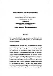
Classification of Problems We will now characterize the problems by various properties. The first and most simple distinction is made according to the characteristic changes of functions. It is possible to extract functions for object changes by a horizontal and vertical analysis of this sort of problem. Fig. 2 depicts an example of a horizontal rotation transformation function of a rectangle. Objects can be decomposed to simple squares, triangles, dots or lines. As shown in Fig. 2, all objects consist of triangles, rectangles or hexagons. The second category, topological characteristic changes, specifies the relationships between certain shapes or objects. Topological characteristics are mathematically classified as determining if two object are: (i) distinct, (ii) overlapping, or (iii) contained within one another. Category three specifies the changes of pattern. It is determined if there are any transformation changes concerning the shapes of objects; that is, if an object (e.g. circle) is transformed into another object e.g., in Fig. 6 the square in the left cell above can be associated with the triangle in the left cell below. The fourth distinction concerns the alteration of the number of elements in a problem. Take, for example, Fig. 3, there the number of objects increases. In other words, if there is an implicit sequence of numbers it must be determined whether the number of objects increases or decreases from cell to cell and whether this change happens horizontally, vertically, or in both directions. A further distinction concerns the characteristics of different shapes. To be analyzed is whether lines, dots, dashes, or other characteristics act in compliance with Boolean functions such as, AND, OR, and XOR. Category number 6 – number of parts – characterizes how many parts the objects are composed of. The following categories horizontal function, vertical function and horizontal-vertical function classify the problems according to the objects of the horizontal/vertical succession of changes. This refers to whether the objects in the cells are dependant upon addition and/or subtraction or only succession. One aspect is rotation, indicating if at least one of the objects is rotated during the changes of the cells. Another aspect takes moving objects into account, this is true if at least one object is moving (e.g., clockwise or counter-clockwise, up, down, or left or right movements of an object). Then, the overall dimension characterizes whether the underlying

Figure 2: An example for a problem in which the functions of change can be extracted horizontally. problem can be solved horizontally or vertically alone (onedimensionally) or requires both (two-dimensionally).

General Categories The classification items for matrix reasoning problems, as discussed above, can be grouped into three main types, which we denote as (i) geometric operation problems, (ii) Boolean operation problems, and (iii) grouping problems.

Figure 3: An example for a problem in which objects are added vertically and horizontally.

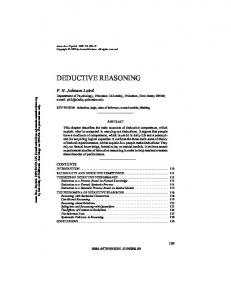
Type 1: Geometric Operation Problems. Problems of this type can be solved by the application of geometric functions which have to be applied on each successive cell (horizontally, vertically or in both directions). Examples for such functions are: • Continuous changes by affine transformations. An example are rotations (e.g., the rectangle is rotated in Fig. 2) or changes in size (scaling). • Addition or removal of objects. An example is the star in the leftmost column in Fig. 3. In each successive cell an additional star is inserted (linear). • Movement of objects (e.g., the triangle and the hexagon in Fig. 2) Type 2: Boolean Operation Problems. To solve problems of this type it is necessary to consider information from at least two cells in relation to a resulting cell. An example for such an underlying functions is the Boolean function XOR (see Fig. 1 and Fig. 7). Type 3: Grouping Problems. This type of problems requires the identification of groups of objects. The pattern changes cannot be solely identified through a determination in the horizontal, the vertical or in both directions. One must consider all cells in order to group features and figure out what is absent or does not occur as frequently as others objects. An example for such a kind of problem is Fig. 4. There are three groups of objects consisting of L, N and X with differences in color, size, shape. The reasoner has to identify the missing object and its characteristic property.

Mathematical Foundation In theoretical computer science the difficulty of a problem is determined with respect to the resources necessary to solve

Figure 4: An example for a grouping problem. The reasoners’ task is to identify three groups of objects. it. A central aspect is the use of computational models (e.g. the Turing machine) to determine the amount of resources necessary to solve the problem. Central to matrix problems are functions mapping one cell to another cell. For this reason, we introduce a complexity measure based on functions, which we can correlate, in the next section, to empirical findings.

Mappings between matrices Most common geometric transformations are linear, including rotations, scaling, shearing, and reflection. In two dimensions, linear transformations can be represented using a 2 × 2 transformation matrix. These transformations (rotation, scaling, i.e. enlarging or shrinking, etc.), can, along with other basic mappings, be defined as basic transformations pi . The cost for a single problem is computed by summing up all transformations which must be applied and the associations which must be built between the stimuli. The complexity of a single association depends on the number of stimuli in each field and the number of transformations between the associated stimuli. See Fig. 2 for an example of computing the costs for rotating the rectangle.

The costs of a basic transformation can be weighted according to the different types of transformation. For example: A translation of a stimuli might be easier to transform as a rotation. So the translated transformation gets a basic cost of 1 unit and the rotation a cost of 2. For the problems listed in Table 1 nine basic transformations were used: identity function (with a cost of 0), translation (1), scaling (1), change in fill-in/background of a stimulus (1), addition and removal of a stimulus (1 each), rotation (2), rotation of the fill-in/background of a stimulus (3) and a change of the type of a stimulus (for example: transforming a triangle into a square, 4). Without weights, all transformations receive a basic cost of 1. Figure 6: An example of a more complex transformation problem. The reasoner has to keep track of changes both horizontally and vertically.

Figure 5: A simple transformation problem as it requires only the horizontal identification of each association between the objects. To solve problem 5 three horizontal associations are required. The different types of the stimuli (line, rectangle, triangle) make it easy to identify the associations. The building of associations follows a hierarchy based on the attributes of a stimulus. In this problem the preferred direction of movement is horizontal, by association of the rectangle in field one with the rectangle rotated 45 degrees in the field to the right, and not vertical where the rectangle could be associated with the triangle below, which has the same degree of rotation and differs only in type. The costs of the three associations are computed by summing up the costs of the different transformations between the members of each association (cell 1 compared with cell 2, cell 2 compared with cell 3 and finally cell 1 compared with cell 3). In this case each association gets a cost of 2 (1 without weights) for applying one rotation. To determine the stimulus in the answer box one additional 45-degree-rotation must be applied to the lower, central triangle. The total costs for this problem are six (costs for all associations) plus two (costs for applied rotation) making eight. Problem 6 shows the difficulty of correct association building. Due to the fact that each field contains two stimuli, they have to be compared to each other to identify the associations. For example taking the white square in the first field and go-

ing the horizontal way, we have to decide weather we associate it with the black square or the shaded rectangle. Therefor the attributes of both stimuli have to be compared with the ones of the white square. Again, the hierarchy of attributes plays an important role, because these stimuli are associated with each other. It depends on which share the highest ranked attribute and not the most attributes. The number of comparisons which have to be performed to identify an association are added to the transformation costs of an association. Once the stimuli are associated to each other, the transformation between them have to be applied on the unassociated stimuli (In this case the white triangle and the shaded rectangle) to determine the stimuli in the answer field. There it is necessary to find the right pairs of stimuli, so that the white triangle changes its color to black and not the shaded circle. Overall it becomes obvious that the difficulty in this problem is raised by the complex relations between the stimuli and this relations can be described as transformations and comparisons on the attributes of the stimuli.

Complexity Measure (Type 1 Problems) We now introduce a more formal notation of this complexity measure. Here pi represents the basic transformation mapping of object on (i) in cell i to on ( j) in cell j. Then the unweighted difference between cell i and cell j is the sum of all basic transformations. The weighted difference formula is derived by adding each weight ai of each basic function pi (mathematically this is expressed by forming the sum of all weights of all basic functions pi ):

∑ ai

(1)

pi

Complexity Measure (Type 2 Problems) Is it possible to apply the same cognitive complexity functions used for Type 1 to problems describing Boolean functions? A Boolean function like the exclusive or (short: XOR)

Table 1: Evaluation of our cognitive complexity measure for a sample of CFT3-problems. Index P denotes the empirical measure from the manual (Weiss, 1971) and give the mean correctness in percent. Cw are the cognitive complexity costs with weights and C0 are the costs without weights. Problem CFT3-A-1-3-1 CFT3-A-1-3-6 CFT3-A-1-3-7 CFT3-A-2-1-1 CFT3-A-2-1-3 CFT3-A-2-1-4 CFT3-A-2-3-2 CFT3-A-2-3-3 CFT3-A-2-3-5 CFT3-A-2-3-6

?

Index P 76 93 78 96 95 90 94 90 47 85

Cw 8 13 18 5 6 4 10 4 26 21

C0 7 10 10 3 3 4 6 4 18 17

Figure 7: An example for a simple XOR problem. can be represented by truth tables: P 0 0 1 1

Q 0 1 0 1

P XOR Q 0 1 1 0

The solution for the problem in Fig. 7 requires the identification of a Boolean XOR function. If the middle cell in the leftmost column (identified by the matrix coordinates (1, 2)) is compared with the middle cell of the same row (2, 2) and both are compared with the middle cell in the rightmost column (3, 2) once can deduce that if the same object (triangle) can be found in the left and middle cell it is not found in the rightmost cell (so it will be deleted). And, whenever there is an object only in the leftmost or middle column (e.g., the star in the same row) it is found in the rightmost cell. These kinds of functions are certainly not as easily recognizable as rotations or scaling and must be defined as such. Feldman (2000) argues that the number of combinations of Boolean functions determines the reasoning difficulty. A position which has recently been questioned (Vigo, 2006; Goodwin, 2006).

Evaluating the Complexity Measure We compare the performance of our complexity measure to some experimental findings with human subjects. First, the complexity measure is able to explain the reasoning difficulty of Type 1 problems. Especially rotating, scaling, movement, position changing, and linear transformations of objects can be well described with our complexity measure. The empirical classification of CFT (Weiss, 1971) problems can be seen in Table 1. The correlation for this complexity function with the empirical data is significant for both: with weight r = −.74, p < .01 and without weight r = −.72, p < .05.

Table 2: Evaluation of our cognitive complexity measure for problems from Lovett et al. (2009). Nr. = problem number, Correct = correctness in percent, Time = mean solving time in seconds, C0 = complexity measure (cf. sum in Equation 1). Nr. 1 2 3 4 5 6 7 8 9 10

Correct 100 100 100 76 100 97 100 100 100 82

Time 10.8 7.3 6.7 8.7 13.4 8.5 6.1 6.1 6.0 23.6

C0 2 1 1 1 1 1 1 1 1 2

Nr. 11 12 13 14 15 16 17 18 19 20

Correct 100 97 91 94 97 100 56 91 82 97

Time 5.8 4.5 5.7 12.3 6.4 5.4 26.7 10.5 6.1 10.8

C0 1 1 2 1 1 1 3 1 1 2

A complexity measure with problems from Evans (1964) was reviewed by Lovett and colleagues (2009). The comparison between our measurement is depicted in Table 2. The correlation between the number of correctly answered problems with our complexity measure is r = −.62, p < .01. The reason for the negative correlation is due to the point that the smaller our complexity measure is, the easier the problem is. Correlation with the solution time between both is r = .67, p < .001.

General Discussion The presented cognitive complexity measure for matrix problems allows the classification of problems with respect to the number of basic functions needed to solve them. This measure is based on abstract ”units” and might have a cognitive counterpart: Nevertheless, it can predict problem difficulty for Type 1 problems and pose a general enough framework for Type 2 and Type 3 problems. What are the differences to existing measures? Our approach is a combination of the-

oretical computer science techniques with ideas going back to the Evans Analogy program (Evans, 1964). It integrates ideas from Kolmogorov complexity (Chater, 2000; Li & Vitanyi, 1997), as it determines complexity based on the minimum number of functions necessary to describe the reasoning difference. Feature extraction and object recognition are basic operations that are required for solving matrix problems. Humans are amazingly accurate and fast at this. However, it is still unknown how humans decide to decompose images of matrix sequences into smaller compounds or treat these images as single objects. Representational Distortion theory can help answer this question by providing a measure for total dissimilarity. Humans might compute these decompositions only for objects that are at least somewhat similar (Müller et al., 2009). The task of feature extraction is difficult because the exact number and set of features that are necessary to extract is not known in advance. Furthermore, the salient features important for the transformation vary heavily from problem to problem. The object transformation results in feature differences that can be classified in two categories. First, objects can change their visibility during the sequence, i.e. they exist in a matrix cell or not. Second, geometric transformations result in changes of position, rotation and scale. Objects for which no transformation can be computed must be treated as separate objects. Nevertheless, humans do not simply check the cells line by line or cell by cell, they can easily shift their reference frame from global to local features and back. One can assume that for an overall first impression the whole problem will be inspected globally, which triggers the next step. The first phase (inspection phase) gives a hint as to how to proceed with the problem and which functions should be chosen in order to successfully solve it. A simply local feature extraction cell by cell can, in many cases, lead to the solution, especially for Type 1 problems (see, Fig. 3). However, this strategy fails if one has to solve Type 3 problems. For this type it is more efficient to examine the problem more globally to discover the required features (see Fig. 4). While Feldmans (2000) approach focuses on which (Boolean) functions to use, we concentrate on the number of function applications. Both approaches together may form a more complete notion of cognitive complexity.

Acknowledgement This research was partially supported by the DFG (German National Research Foundation) in the Transregional Collaborative Research Center SFB/TR 8 within project R8[CSPACE] and by a Steinbuch-Stipend to the second author.

References Binet, A., & Simon, T. (1905). The development of intelligence in children. L’ Annee psychologique, 12, 191–244. Carpenter, P. A., Just, M. A., & Shell, P. (1990). What one intelligence test measures: A theoretical account of the processing in the raven progressive matrices test. Psychological Review, 97(3), 404–431.

Cattell, K., & Cattell, A. (1959). Culture fair intelligence test. Institute for Personality and Ability Testing. Cattell, R. (1968). Are IQ tests intelligent? Psychology today, 1(10), 56–62. Chater, N. (2000). The logic of human learning. Nature, 407, 572-573. Chater, N., & Hahn, U. (1997). Representational distortion, similarity and the universal law of generalization. In Proceedings of the similarity and categorization workshop 97 (pp. 31–36). University of Edinburgh. Evans, T. G. (1964). A heuristic program to solve geometricanalogy problems. Air Force Cambridge Research, Laboratories (OAR) Bedford, Massachusetts. Eysenck, H. J. (1962). Know your own I.Q. Penguin, Harmondsworth, Middlesex. Feldman, J. (2000). Minimization of boolean complexity in human concept learning. Nature, 407, 630–633. Goodwin, G. P. (2006). How individuals learn simple boolean systems and diagnose their faults. Princeton University. Hahn, U., Chater, N., & Richardson, L. B. (2003). Similarity as transformation. Cognition, 87(1), 1–32. Li, M., & Vitanyi, P. (1997). An introduction to Kolmogorov Complexity and its Applications. Springer. Lovett, A., Tomai, E., Forbus, K., & Usher, J. (2009). Solving geometric analogy problems through two-stage analogical mapping. Cognitive Science, 33 (7), 1192–1231. Müller, M., van Rooij, I., & Wareham, T. (2009). Similarity as tractable transformation. In N. Taatgen & H. van Rijn (Eds.), Proceedings of the 31st Annual Meeting of the Cognitive Science Society (pp. 49–55). Newell, A., & Simon, H. A. (1972). Human problem solving. Englewood Cliffs, NJ: Prentice-Hall. Raven, J. C. (1962). Advanced Progressive Matrices, Set II. London: H. K. Lewis, (Distributed in the United States by The Psychological Corporation, San Antonio, TX). Raven, J. C., Raven, J. C., & Court, J. H. (2000). Manual for Ravens Progressive Matrices and Vocabulary Scales. Oxford: Oxford Psychologists Press. Russell, K., & Carter, P. J. (1994). IQ Firepower. Robinson Publishing, London. van Rooij, I. (2008). The tractable cognition thesis. Cognitive Science, 32, 939-984. Vigo, R. (2006). A note on the complexity of boolean concepts. Journal of Mathematical Psychology, 50(5), 501– 510. Wechsler, D., Hardesty, A., Lauber, H., & Bondy, C. (1961). Die Messung der Intelligenz Erwachsener: Textband zum Hamburg-Wechsler-Intelligenztest für Erwachsene (Hawie). H. Huber. Weiss, R. H. (1971). Grundintelligenztest Skala 3 - CFT 3. Stuttgart.