estimating complexity of classification tasks using ... - CogniMem

Ivan Budnyk, Abdennasser Chebira, Kurosh Madani / Computing, 2009, Vol. 8, Issue 1, 43-52

[email protected] www.computingonline.net

ISSN 1727-6209 International Scientific Journal of Computing

ESTIMATING COMPLEXITY OF CLASSIFICATION TASKS USING NEUROCOMPUTERS TECHNOLOGY Ivan Budnyk, Abdennasser Chebira, Kurosh Madani Images, Signals and Intelligent Systems Laboratory (LISSI / EA 3956) PARIS 12 – Val de Marne University, Senart-Fontainebleau Institute of Technology, Bat. A, Av. Pierre Point, F-77127 Lieusaint, France, {ivan.budnyk, chebira, madani}@univ-paris12.fr, http://lissi.univ-paris12.fr Abstract: This paper presents an alternative approach for estimating task complexity. Construction of a self-organizing neural tree structure, following the paradigm “divide and rule”, requires knowledge about task complexity. Our aim is to determine complexity indicator function and to hallmark its’ main properties. A new approach uses IBM © Zero Instruction Set Computer (ZISC-036 ®) and applies for a range of the different classification tasks. Keywords: IBM © Zero Instruction Set Computer (ZISC-036 ®) Neurocomputer, Neural tree modular architecture, TDTS, DNA (Deoxyribonucleic acid), RNA (Ribonucleic acid), exon, intron, Splice junctions problem, Tic-tac-toe endgame problem.

1. INTRODUCTION In this paper we present an alternative complexity estimating approach for a modular neural tree structure. This structure uses key module of the complexity estimation for solving classification problem following the paradigm “divide and rule”. This general modular tree structure [1 ] is Tree Divide To Simplify (T-DTS) Fig. 1. Complexity reduction is the key point on which the modular approach acts. Complexity reduction performs not only at the problem’s solution level but also at the processing procedure’s level. The main idea is to reduce the complexity by splitting a complex problem into a set of simpler sub-problems: this leads to “multi-modeling” where a set of simple models is used to sculpt a complex behavior. Thus, one of the foremost functions to be performed is the complexity estimation. We introduce in this paper the complexity which is based on ZISC-036 ® neurocomputer [2]. Before describing the proposed approach, we present in the second section T-DTS paradigm and the hardware tool used for complexity estimation, IBM © Zero Instruction Set Computer (ZISC-036 ®). Third section properly contains the description of a new approach. A validation and a definition of the classification complexity contain section four. Obtained results and their overview are presented in the sections five. Final section presents conclusion

and further perspectives of the work.

2. THE NEURAL STRUCTURE AND NEUROCOMPUTER In a very large number of cases dealing with real world dilemmas and applications (system identification, industrial processes, manufacturing regulation, optimization, decision, pattern recognition systems, plants safety, etc), information is available as data stored in databases [3]. An efficient data processing becomes a chief condition to solve problems related to above-mentioned areas. The use of machine learning approaches for such problems can be justified in the following way [4]: • machine learning approaches produce predictable models with comparable and often superior quality than models based on the statistical analysis. • they are more easy to understand, intelligible to human beings. • instead of trying to fit the data to the model, most of machine learning approaches build models by including a knowledge that will accommodate all cases in the sample population. Real life models can be sometimes approximated with mathematical models (liner or non-linear), but sometimes that is not possible. • machine learning approaches offer better solution when the knowledge describing the real life

43


world is incomplete, inexact, and imprecise. An issue of using machine learning approaches is a capability to model complexity reduction by splitting a complex problem into a set of simpler sub-problems: multi-modeling, where a set of simple models, is used to sculpt a complex behavior [5] [6]. For such purpose, a tree-like splitting process, based on complexity estimation, divides the problem’s representative database on a set of sub-databases, constructing a specific model (dedicated processing module) for each sub-database. That leads to a modular tree-like processing architecture including several models. In order to deal with real word problem, we propose, a modular approach based on divide and conquer paradigm [1] [3]. In this approach, Tree Divide To Simplify or T-DTS, we divide a problem into sub-problems recursively and generate a neural tree computing structure. Data (D), Targets (T)

Preprocessing (Normalizing, Removing Outliers, Principal Component Analysis) (PD) - Preprocessed Data Targets (T) Complexity Estimation Module Learning Phase Feature Space Splitting NN based Models Generation

Structure Construction

P – Prototypes NNTP - NN Trained Parameters Operation Phase

Processing Results

Fig. 1 - General bloc diagram of T-DTS.

T-DTS and associated algorithm(s) construct(s) a tree-like evolutionary neural architecture automatically where nodes, call “Splitting Units”, are decision units and leafs, call “Neural Network based Models”, correspond to neural based processing units [6] [7] [8]. T-DTS includes two main operation modes. The first is the learning phase, when T-DTS system decomposes the input database and provides processing sub-structures, and tools for decomposed sets of data. The second phase is the operation phase. Fig. 1, gives the general bloc diagram of TDTS operational steps. Fig. 1 shows that T-DTS could be characterized by four main blocks: “data pre-processing”, “learning process”, “generalization process”, “complexity estimation module”. The tree structure construction is based mainly on the complexity estimation module. This module introduces a feedback in the learning process and control the tree

44

building process. The reliability of tree model to sculpt the problem behavior is associated mainly to the complexity estimation module. This work focuses on the aspect of complexity estimation and proposes a new approach based on neurocomputer hardware ZISC-036 ®: IBM © ZISC-036 ® neuron-computer is a fully integrated circuit based on neural network designed for recognition and classification [2] [6] [9]. It is a parallel neural processor based on the Reduced Coulomb Energy (RCE) [10] and K-Nearest Neighbor (KNN) [11] algorithms. Each chip is the implementation of the RBF-like model [12]. RBF approach could be seen as mapping an Ndimensional space by prototypes. Each prototype is associated with a category and an influence field. ZISC-036 ® system implements two kinds of distance metrics that we have used L1 and LSUP respectively. The first one, L1 corresponds to a polyhedral volume influence field and the second LSUP - to a hyper-cubical one. During estimation complexity the RCE is used. This hardware implemented method on ZISC-036 ® is effective in separating patterns classes by nonlinear boundaries. However, the RCE network depends on the user-specified parameters which are computationally expensive to optimize [10]. Each ZISC-036 ® neuron of the network is an element, which is able to: memorize a prototype composed of 64 components, the associated category, an influence field and a context, compute the distance and compare basing on the selected norm L1/LSUP between its memorized prototype and the input vector, interact with other neurons adjusting their influence fields during learning phase in order to find the minimal distance, category, etc. The next section presents a complexity estimation approach that is based on such neurocomputer’s capabilities.

3. COMPLEXITY ESTIMATION APPROACH It is clear that the efficiency of neural network models is the basic precondition of their practical applicability in the artificial intelligence. With respect to the fact that neural networks models were inspired by living organisms which perform the relevant function efficiently, this approach leads to the complexity-theoretic definition of intelligence: the way of efficient knowledge representation. We can understand the efficiency in three senses: an efficient creation and adaptation of this representation (learning complexity), its memory demands (descriptive complexity) and efficient


knowledge retrieval (computational power). [13] The complexity estimating in T-DTS is used to understand the behavior of classifiers. A chief aim of the complexity estimating is to check, to measure the difficulty of a classification task before proper processing and to construct an optimized modular tree-like system. The definition of the classification complexity as a complexity in general term relates the difficulty in formalization of the whole compared to that of its fundamental parts (from the point of view of the language). It is only applicable in cases where there is at least a possibility of gaining almost complete information about the components, thus clearly separating ignorance from complexity. We have different concepts of complexity depending on the base language chosen, the type of difficulty focused on and the type of formulation desired within that language [14]. In our work we determine a complexity as the amount of computational resource that it takes to solve a classification problem. Thus, a complexity here is the related to the amount of the resource supplied. Thus way of defining complexity as a computing complexity of classification is adopted for our approach, because of hardware limitation of the classification tools [15]. Supposing a classification problem has a collection of m objects of database associated to labels/categories. We classify and estimate the classification complexity using the neurocomputer without regard to a classifier. Firstly, we learn the ZISC-036 ® neurocomputer to classify objects using the associated database. Then estimate the task computational complexity, analyzing the generated ZISC-036 ® neural network structure that has been created by this neurocomputer. In general, we expect that a method which satisfying demands of the classification method will involve a more complex structure for a more complex problem, or being more precisely, the neural network structure will be an archetypal platform for extracting underlying properties/parameters of the classification complexity [16]. The simplest neural network structure feature is the number n of neurons created during the learning phase. The following indicator is defined (1), where parameter n is a value that reflects complexity and m – database size that have been used to train neural network structure: Q=

n , m ≥ 1, n ≥ 0 m

(1)

We suppose that there exists some function of complexity n=g(.) ,where the arguments of it may be the signal-to-noise ratio, the dimension of the

representation space, boundary non-linearity and/or database size. In a first approach, we consider only g(.) function’s variations according to m axis: g(m). We suppose that our database (e.g. the used database) is free of any incorrect or missing information. On the basis on gp(m), where p is vector of parameters, a complexity indicator Qp defines: Q p ( m) =

g p ( m) m

, m ≥ 1, g p ( m ) ≥ 0

(2)

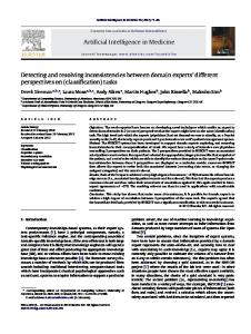
We expect that for the same problem, as we enhance m, the problem seem to be less complex: more information reduces problem ambiguity. On the other hand, for problems of different and increasing complexity, an evolution of Qp indicator should have a relevant trend. Also we can interpret obtained structure of neurons as the result of computational process [17]. The process consists of a program plus data. This idea underlies efforts to define both classical algorithmic complexity (eg. Chaitin, Kolmogorov [13]) and information entropy (eg. Papentin, Brooks). Most definitions of this kind (eg. Gramma, Bennett’s and Logren’s complexity [14]) hinge on the notion of the shortest program. This idea is unworkable in practice because in general we cannot prove that a particular program is the shortest. An alternative point of our approach is a computing of the complexity in the context [17]. Of course, this is another definition of computational complexity [18]. However, the strong feature of this definition is a strong orientation on the limitation of computational capabilities. In order to check the behavior of the indicatorfunction (2), we have defined a specific bench-mark and applied extracted approach to DNA, Tic-tac-toe classification problems present in the following sections. Specific benchmarking database. Basically, we construct 5 databases representing a mapping of a restricted 2D space to 2 categories, Fig. 2. Each pattern is divided into two and more equal striped sub-zones, each of them belonging to the categories 1 or 2 alternatively. In learning phase we create samples using randomly generated plots (objects) with coordinates (x,y). The number of samples m, in our case of uniform random distribution, naturally has an influence on the quality of the striped zones (categories) demarcation. According to the value of the first coordinate x, and according to the amount of the striped sub-zones, the appropriate category c is assigned to the sample, and such structure (xj ,yj, cj) sends to neurocomputer on the learning.

45


Fig. 2 – Test patterns.

The second phase is classification or in the other words real testing of the generalizing ZISC-036 ® neurocomputer abilities. We again, randomly and uniformly, generate m samples and their associated category. Gaining classification statistics, we compute the indicator-function Qp. DNA patterns classification problem. Deoxyribonucleic acid (DNA) is a nucleic acid that contains the genetic instructions for the development and function of living organisms. This is two long strands entwine like vines, in the shape of a double helix.

Fig. 3 – Genes DNA (black) transcription into RNA in the nucleus of the cell.

The major function of DNA is to encode the sequence of amino acid residues in proteins, using the genetic code. To read the genetic code, cells make a copy of a stretch of DNA in Ribonucleic acid (RNA) [19]. These RNA copies can then be used to direct protein synthesis [20] [21]. During the protein creation in higher organisms take a place a process of elimination of the superfluous DNA sequence. Points on a DNA sequence at which redundant DNA is removed calls splice junctions. The problem posed in this dataset is to recognize,

46

given a sequence of DNA, the boundaries between exons (the parts of the DNA sequence retained after splicing) and introns (the parts of the DNA sequence that are spliced out). This problem consists of two subtasks: recognizing exon/intron boundaries (referred to as EI sites), and recognizing intron/exon boundaries (IE sites). (In the biological community, IE borders are referred to an “acceptors” while EI borders are referred to as “donors”.) For our complexity estimation purpose we use molecular biology database titled as “Primate splice-junction gene sequences (DNA) with associated imperfect domain theory” donated by G. Towell, M. Noordewier, and J. Shavlik that is available in Machine Learning Repository of Bren School of Information and Computer Science University of California, Irvine (ftp site: ics.uci.edu) This benchmark data has the following main features: All examples taken from Genbank 64.1 (ftp site: genbank.bio.net) Number of Instances: 3190 Number of Attributes: 62 Missing Attribute Values: none Class Distribution: EI: 767 (25%) IE: 768 (25%) Neither: 1655 (50%) We create on the learning phase file(s) that consist of the samples randomly chosen from database. The number of samples m, in this case is the amount of instances. Each instance has a category c and 60 sequential DNA nucleotide positions aj (0 < j < 61) and in this case the structure (aij , ci) where i is the sample number which is sent to neurocomputer on the learning. The second classification phase is identical to bench-mark testing. We generate m samples (instances) and their associated category, than compute the indicator-function Qi. Difference between those two bench-mark examples is that the probabilities of coincidence are different, because of different database size and classes’ distributions. Moreover, the sequence of DNA encoded in aj reflects a part of 3D (not 2D) space of a DNA double helix.

Tic-tac-toe endgame classification problem The tic-tac-toe endgame dataset encodes the complete set of possible board configurations at the end of tic-tac-toe games, where “x” is assumed to have played first. The target concept is “win for x” (i.e., true when “x” has one of 8 possible ways to create a “three-in-a-row”). The dataset contains 958 instances without missing values, each with 9 attributes, corresponding to tic-tac-toe squares and taking on 1 of 3 possible values: “x”, “o”, and “empty”.


From the view of data structure the tic-tac-toe endgame problem is similar to DNA patterns recognition, that’s why technically we easy apply identical approach for learning and classification. Moreover, tic-tac-toe problem “seems to be” simpler from the data size view. There are only 2 classes. Each array of attributes is shorter at least in 6 times. Every attribute has twice less variants of the value, plus it is 2D space. In next sections, especially section 6, we show delusiveness of such assumption.

behavior of a complexity of learning [22] as m becomes large. Since the curve can be used to determine how large m must be before the other parameters of classification such the rate of success reach a desire value.

4. APPROACH VALIDATION To validate proposed approach we have conducted the experimentations with the following settings: two IBM © ZISC-036 ® modes: LSUP/L1; five different databases with increasing complexity; eight variants of m value: 50, 100, 250, 500, 1000, 2500, 5000, 10000. For each set of parameters, tests are repeated 10 times in order to get statistical average and to check the deviations of the tests Totally, 800 tests have been performed. Fig. 4, Fig. 5, shows the charts of Qi where i is the database index or pattern index. We expect that Q5 for 10 sub-zones reaches a higher value than Q1. Intuitively the problem corresponding to classification of 10 stripped sub-zones (Q5) is more complex than for 2 (Q1).

Fig. 5 – Coefficients of complexity Qi(m) - L1 ZISC036 ® mode.

The chart analysis suggests that exist(s) a point(s) mj such as: ∂2 Qi (m j ) = 0 ∂ ( m)

(3)

At such point mj we have the following properties: ∀m ≥ 1, ∃ε j > 0 : ∀m ∈ (m j − ε j ; m j ) ⇒

∂2 ∂2 Qi (m j ) < 0, ∀m > m j ⇒ Qi ( m j ) > 0 ∂ ( m) ∂ ( m)

(4.1)

or

∀m ≥ 1, ∃ε j > 0 : ∀m ∈ (m j − ε j ; m j ) ⇒ ∂2 ∂2 Qi ( m j ) > 0, ∀m > m j ⇒ Qi ( m j ) < 0 ∂ ( m) ∂ ( m)

(4.2)

It means that there exists one or more point(s) mj where the second derivative of Qi changes its sign. Then we are interesting in m0 defined by: m 0 = max( m 1 ,.., m j ,... m k ) m 1 < .. < m

Fig. 4 – Coefficients of complexity Qi(m) - LSUP ZISC-036 ® mode.

Consider a simple concept of view on the complexity of the learning process, in which a neurocomputer attempts to build complex neural structure in order to infer an unknown classifying concept, so regarding this process, Qi(m) is a complexity learning curve. The values of Qi(m) are clearly closely related to each other. In either measuring we are interesting in the asymptotic

j

< ... < m k , m 0 = m k

(5)

Where k is the number of points mj. Main characteristic of the point m0 is: ∀m > m 0 : m → +∞ ⇒ Qi ( m ) → const (6) In general case const ≥ 0. The feature of the second derivative sign changes presents on the chart of the rates of the success classification, Fig. 6. That supports the idea of the strong influence second derivate has on the complexity estimation task. That fact turns a look on the problems not from the quantity side of complexity, but from the quality one. It is clearly seen that in our specific bench-mark examples, the complexity of the classifying is lying

47


in the range from Example 1 (2 zones, the easiest case) to Example 5 (10 zones, the complex one).

been generated from the given database in order to test, get good average parameters and to check the deviations. Approximately, up to 8400 tests have been performed. After cubical polynomial approximation for 3 different initial modes we compute the coefficients of complexity Qi(m0) Fig. 7.

Fig. 6 – Rates of success of classification. Examples 1 – 5. LSUP ZISC-036 ® mode.

Analysis of the plots m0,Q1 (Example 1) till m0,Q5 (Example 5) for related classification tasks implies the following property: m0,Q < m0,Q < m0,Q < m0,Q < m0,Q (7) In our particular tests we have (8), mentioning that in general (5), (7) and (8) are not obvious. 1

2

3

4

5

Q1 ( m 0 ) < Q 2 ( m 0 ) < Q 3 ( m 0 ) < < Q 4 (m 0 ) < Q5 (m 0 )

(8)

On the other hand, we consider a particular value of m (an interesting value is m0 for which the second derivative of Qi (m) changes the sign) stating Qi(m0) acting as a “complexity coefficient”. In our case, Qi(m0) acts as a critical checkpoint of classification process. The increase of m0 stands for the classification task’s complexity increasing. Actually, many researchers try to identify general feature(s) of self organizing processes, so there is no revolutionary new in our approach. In particular [23], we point out that in many emergent and self-organizing processes, phase changes (from local to global behavior) occur at a well-defined critical value of some order parameter. For example, water freezes at a fixed temperature, nuclear chain reactions require a critical mass of fuel. So in next section we search the critical point(s) which in our approach represents its’ complexity.

5. RESULTS For DNA patterns recognition, we generate the 100 (amounts of the test) pairs (for learning and classification phases) of the files. For each set of the global parameter such as m, ZISC-036 ® mode, etc. appropriate pairs of the data files randomly have

48

Fig. 7 – Evaluation of Qp(m) for DNA sequences recognition for different initializing parameter p, maximal influence field (MIF) of ZISC-036 ® : Q55(m), Q56(m), Q4096(m) modes.

The Table 1 represents the summary of the obtained chart results. Global optimizing parameter MIF is a maximum influence field used to initialize the RCE algorithm. Table 1. Coefficient of complexity for DNA sequences recognition Initial mode MIF 55 MIF 56 MIF 4096

m0 730 775 700

Qi(m0) 0.618 0.561 0.104

Fig. 8, Fig. 9, Fig. 10 supports the idea of the strong influence of the second derivate feature on the complexity estimation on the quality level of the recognitions. For example on the Fig. 9, for calculated m0,Q56 = 775 we can generally observe for m > m0,Q56 the rates of success classification has a strong tendency to increase and the rates of failure – decrease. For m greater than critical m0,Q55 the rate of uncertainty (the rate of the patterns, which cannot be classify by hardware tool, put to the special category) strongly concentrate around 14% The mentioned supports that Qp(m0) is the coefficient of the task complexity. Constructing cubical approximation for Qp(m) and calculating this coefficient for the best satisfying the initial ZISC-036 ® parameter is MIF = 56. The obtained rate of the success classification is 53.5%. The rate of failure – 15.6% are satisfied knowing


[21] that even using improved RBF methodology we cannot reach more than 66.3% of successful DNA pattern classifying [24]. That is why computed coefficient of complexity Q56 = 0.561, where m0,Q56 = 775 Fig. 7, is acceptable and expected. Problem of DNA pattern classifying seems to be a priori complex.

Fig. 10 – Rates of success, failure and uncertainty of classification for Q4096 (m).

The tic-tac-toe classification problem from the point of view of the covering type of algorithms is difficult [26] Fig. 11, as well as it is difficult for the methods based on the approach divide and conquer [27]. Fig. 8 – Rates of success, failure and uncertainty of classification for Q55(m).

Fig. 11 – A covering family of algorithms applied for the tic-tac-toe classification problem.

Fig. 9 – Rates of success, failure and uncertainty of classification for Q56(m).

The same experimental protocol as for DNA benchmark is used for tic-tac-toe endgame problem. The datasets from the UCI machine learning repository is taken [25]. The database is randomly divided as in the reference sources into learning (90% of data) and recognition (remaining 10% of data) sets and to be comparable to the previous range of tests we also divide database on 50% of data for learning and 50% - for classification. The tests are applied to the training sets and this process is repeated 32 times for each data set (a pair of data files). We change during a testing a tuning initializing parameter MIF, so totally we performed around 1728 tests.

Another group of methods, which use the idea of finding minimal description function and its’ approximation for the class of the examples, are proven [28] to be NP-complete. Generally, the class of problems such as DNA patterns and tic-tac-toe endgame recognition are time and resource consuming and in some cases even impossible to examine all possible examples. Table 2 contains the summary of the obtained chart results. Relatively optimal tuning factor of classification is MIF = 3. Even for this optimal initial parameter the rate of the successful classification reaches by default level 65% [26]. Table 2. Coefficient of complexity for tic-tac-toe endgame problem Initial mode MIF 3 MIF 56

m0 545 522

Qi(m0) 0.6384 0.0839

Coefficient of complexity Q3(m0) = 0.6384 In fact, tic-tac-toe problem for the proposed method of the classification is the most complex. We can state so, because the other parameters as sample distribution (the main of them) are equal for DNA pattern classification and tic-tac-toe endgame

49


problems.

are shown on Fig. 13 and Fig. 14.

6. CONCLUSION

Fig. 12 – Evaluation of Qp(m) for tic-tac-toe endgame problem for different initializing parameter p, maximal influence field (MIF) of ZISC-036 ® : Q3(m), Q56(m), modes.



The rates of the classification process for not optimal parameter MIF = 56, and optimal MIF = 3

50

In this paper we describe a new method for complexity estimation based on an indicatorfunction related to neurocomputing technology. The complexity indicator is extracted from some pertinent neural network structure parameter - the number of neurons in the structure. The presented approach uses the following hypothesis: more complex classification problem involves more complex neural network structures for its processing relating to the initial condition where the other basic parameters are equal. The presented concept has been implemented on IBM © ZISC-036 ® massively parallel neurocomputer and takes additional advantage of standard digital technology robustness and the high processing speed of this neuroprocessor. It has been validated using a two-classes benchmark set of classification paradigms with increasing complexity. The proposed concept has been applied and verified using a three-class set of DNA patterns and two-class tic-tac-toe endgame classification problem. Future research in this field will embed this approach in T-DTS in order to improve performance. A parallel stream of the development of this approach will be formalization a complexity indicator and specification of the other pertinent parameters to study their properties and their influence on the integrated complexity coefficient.

7. REFERENCES [1] E. Bouyoucef. A. Chebira. M. Rybnik. K. Madani. Multiple Neural Network Model Generator with Complexity Estimation and self-Organization Abilities, International Scientific Journal of Computing (2005) Vol. 4. Issue 3, pp. 20–29. [2] Laboratory IBM France. ZISC® 036 Neurons User’s Manual. Version 1.2. Component Development (1998). [3] K. Madani. M. Rybnik. A. Chebira. Data Driven Multiple Neural Network Models Generator Based on a Tree-like Scheduler. Lecture Notes in Computer Science. Edited J. Mira. A. Prieto. Springer Verlag (2003). ISBN 3-540-40210-1, pp. 382-389. [4] M.A. DE Almeida. H. Lounis. W.L. Melo. An Investigation on the Use of Machine Learned Models for Estimating Software Correctability. International Journal of Software Engineering and Knowledge Engineer (JSEE). Volume 9. Issue 5. (October 1999), pp. 565-593.


[5] M. I. Jordan. L. Xu. Convergence Results for the EM Approach to Mixture of Experts Architectures Neural Networks. Pergamon. Elsevier (1995). Volume 8, N 9, pp. 14091431. [6] K. Madani. A. Chebira. Data Analysis Approach Based on a Neural Networks Data Sets Decomposition and it’s Hardware Implementation. PKDD 2000. Lyon, France 2000. [7] G. DE Tremiolles. Contribution to the Theoretical Study of Neuro-Mimetic Models and to their Experimental Validation: a Panel of Industrial Applications. Ph.D. Report. University of Paris XII (1998). [8] G. DE Tremiolles. P. Tannhof. B. Plougonven. C. Demarigny. K. Madani. Visual Probe Mark Inspection using Hardware Implementation of Artificial Neural Networks in VLSI Production. Lecture Notes in Computer Science, Biological and Artificial Computation: From Neuroscience to Technology. Edited by J. Mira. R. Diaz. M. J. Cabestany. Springer Verlag, Berlin. Heidelberg (1997) 1374-1383. [9] Laboratory IBM France. ISC/ISA Accelerator Card for PC. User Manual. IBM France (1995). [10] J. Wang. P. Neskovic. L. N. Cooper. Learning class regions by sphere covering. IBNS Technical Report 2006-02. March 2006. Department of Physics and Institute for Brain and Neural Systems Brown University. Providence. RI 02912. [11] B. V. Dasarathy, editor (1991) Nearest Neighbor (NN) Norms: NN Pattern Classification Techniques. ISBN 0-8186-89307. [12] J. Park. J. W. Sandberg. Universal Approximation Using Radial Basis Functions Network, Neural Computation (1991) Volume 3, pp. 246-257. [13] J. Sima. R. Neruda. Teoretické Otázky Neuronovỷch Sítí. MATFYZPRESS, Prague(1996), 390 pages. [14] B. Edmonds. What is Complexity? - The philosophy of complexity per se with application to some examples in evolution. F. Heylighen & D. Aerts (Eds.) 1999. The Evolution of Complexity. [15] A. Kohn. L. G. Nakano. V. Mani. A Class Discriminability Measure Based on Feature Space Partitioning. Pattern Recognition (1996) 29(5), pp. 873-887. [16] S. F. Bush. On The Effectiveness of Kolmogorov Complexity Estimation to Discriminate Semantic Types, Senior member of IEEE, Todd Hughes, Ph.D.

[17] D. G. Green. D. Newth. Towards a Theory of Everything? – Grand Challenge in Complexity and Informatics. Complexity international (2000). Volume 8. ISSN 1320-0682. [18] C. Lucas. Quantifying Complexity Theory. (2004). [19] J. Watson. F. Crick. Molecular Structure of Nucleic Acids, a Structure for Deoxyribose Nucleic Acid, Nature (1953) 171 (4356), 737-8. [20] J. M. Butler. Forensic DNA Typing, Elsevier (2001), pp. 14-15. [21] A. Bruce. A. Johnson. J. Lewis. M. Raff, K. Roberts. P. Walters. Molecular Biology of the Cell; Fourth Edition. New York and London. Garland Science (2000). [22] D. Haussler. M. Kearns. R. Schapire. Bounds on the Sample Complexity of Bayesian Learning Using Information Theory and the VC Dimension. Proceeding of the 4th annual workshop on Computional Learning Theory. Santa Cruz. Califonia. U.S. 1991, pp. 61-74. ISBN: 1-55860-213-5. [23] H. Haken. Synergetics. Springer-Verlag, Berlin (1978). [24] E. Bouyoucef, Comparaison des Performances de la T-DTS avec 34 Algorithmes de Classification en Exploitant 16 Bases de Données de l’UCI (Machine Learning Repository). Ph.D. Report. University of Paris XII (2007). [25] D. W. Aha. Incremental Constructive Induction: An Instance-Based Approach. In Proceedings of the Eight International Workshop on Machine Learning. Morgan Kaufmann (1991), pp. 117-121. [26] F. Torre. Contributions à l’apprentissage disjonctif. Intégration des bias de langage à l’algorithme générer-et-tester. Équipe Infèrence et Apprentisage Laboratoire de Recherche en Informatique Université ParisSud. Rapport (28.02.2000), pp. 16-19. [27] H. Bostrom. Covering vs. divide-and-conquer for top-down induction of logic programs. Proceedings of the 14th International Joint Conference on Artificial Intelligence (1995), pp. 1194-1200. [28] L. Dakovski. Z. Shevked. An Alternative Approach for Learning from Examples, International Conference on Computer Systems and Technologies – CompSysTech’ 2005, pp. IIIB.5-1 – IIIB.5-6.

51


Ivan Budnyk received his Specialist of Computer Science degree from the National University of “Kyiv-Mohyla Academy”, in 2004. Since November 2006 he works as Ph.D. student in Images, Signals and Intelligent Systems Laboratory (LISSI / EA 3956) of PARIS XII – Val de Marne University. His research works deals with data processing, artificial learning, complexity estimation methods, classification techniques and parallel programming. Dr. Abdennasser Chebira Received his Ph.D. degree in Electrical Engineering and Computer Sciences from PARIS XI University, Orsay, France, in 1994. Since September 1994 he works as Professor Assistant at Sénart Institute of Technology of PARIS XII – Val de Marne University. He is a staff researcher at Images, Signal and Intelligent Systems Laboratory (LISSI / EA 3956) of this University. His current research works concern selforganizing neural network based multi-modeling, hybrid neural based information processing systems; Neural based data fusion and complexity estimation. Prof. Kurosh Madani received his Ph.D. degree in Electrical Engineering and Computer Sciences from University PARIS XI (PARIS-SUD), Orsay, France, in 1990. From 1989 to 1990, he worked as assistant professor at Institute of Fundamental Electronics of PARIS XI University. In 1990, he joined Creteil-Sénart Institute of Technology of University PARIS XII – Val de Marne, Lieusaint, France, where he worked from 1990 to 1998 as assistant professor. In 1995, he received the DHDR Doctor Habilitate degree (senior research Dr. Hab. degree) from University PARIS XII – Val de Marne. Since 1998 he works as Chair Professor in Electrical Engineering of Sénart Institute of Technology of University PARIS XII – Val de Marne. From 1992 to 2004 he has been head of Intelligence in Instrumentation and Systems Laboratory of PARIS XII – Val de Marne University located at Sénart Institute of Technology. Since 2005, he is head of one of the three research teams of Image, Signal and Intelligent Systems Laboratory (LISSI / EA 3956) of PARIS XII University. He has worked on both digital and analog implementation of processors arrays for image processing by stochastic relaxation, electro-optical random number generation, and both analog and digital Artificial Neural Networks (ANN) implementation. His current research interests include large ANN structures

52

behavior modeling and implementation, hybrid neural based information processing systems and their software and hardware implementations, design and implementation of real-time neurocontrol and neural based fault detection and diagnosis systems. Since 1996 he is a permanent member (elected Academician) of International Informatization Academy. In 1997, he was also elected as Academician of International Academy of Technological Cybernetics.