Email: {oliver.thiergart,emanuel.habets}@audiolabs-erlangen.de. AbstractâThe .... For purely directional sound, using (4) and (9) the PSD. Φdir lm,l'm' is ...
2012 IEEE 27-th Convention of Electrical and Electronics Engineers in Israel
Coherence-Based Diffuseness Estimation in the Spherical Harmonic Domain Daniel P. Jarrett∗† , Oliver Thiergart† , Emanu¨el A. P. Habets† and Patrick A. Naylor∗ ∗ Dept.
of Electrical & Electronic Engineering, Imperial College London, UK Email: {daniel.jarrett05,p.naylor}@imperial.ac.uk † International Audio Laboratories Erlangen, Germany Email: {oliver.thiergart,emanuel.habets}@audiolabs-erlangen.de
Abstract—The diffuseness of sound fields has previously been estimated in the spatial domain using the spatial coherence between a pair of microphones (omnidirectional or first-order). In this paper, we propose a diffuseness estimator for spherical microphone arrays based on the coherence between eigenbeams, which result from a spherical harmonic decomposition of the sound field. The weighted averaging of the diffuseness estimates over all eigenbeam pairs is shown to significantly reduce the variance of the estimates, particularly in fields with low diffuseness.
I. INTRODUCTION The estimation of the diffuseness of a sound field is useful for a number of acoustic signal processing applications. For example, this information can be used in dereverberation algorithms to suppress diffuse reverberant energy while retaining the direct sound [1]. It can also be used to improve the accuracy of source localization algorithms, by eliminating inaccurate direction of arrival (DOA) estimates obtained under highly diffuse conditions. Moreover, the diffuseness represents an important parameter in the description of spatial sound, e.g., in Directional Audio Coding (DirAC) [2]. Diffuseness estimation has previously been accomplished by considering the spatial coherence between a pair of omnidirectional microphones [3] and an arbitrary pair of firstorder microphones [4]. Spherical microphone arrays, typically incorporating a few dozen microphones, enable the analysis of sound fields in three dimensions [5], [6], and have recently been used for speech enhancement applications such as noise reduction [7] and dereverberation [8]. In this paper, we take advantage of the availability of these additional microphone signals, and propose a diffuseness estimation algorithm for spherical microphone arrays based on the coherence between eigenbeams. The eigenbeams result from a spherical harmonic decomposition of the sound field. In the spatial domain, the omnidirectional microphone signals are correlated at low frequencies even when the sound field is purely diffuse, which makes robust diffuseness estimation difficult. An advantage of the spherical harmonic domain (SHD) is that in a purely diffuse sound field, the coherence between the eigenbeams is zero, while in a purely directional sound field (i.e., due to a single plane wave) the coherence is one. We also take advantage of the availability of many eigenbeam pairs to reduce the variance of our estimates.
II. PROBLEM FORMULATION In the following, we work in the short-time Fourier transform (STFT) domain, where k denotes the discrete frequency index and t denotes the time frame index. A. Spatial and Spherical Harmonic Domain Signal Models In the spatial domain, the signal X(k, r, t) received at a microphone position r = (r, Ω) = (r, θ, φ) (in spherical coordinates) is modeled as the sum of a directional signal Xdir , a diffuse signal Xdiff and a sensor noise signal V , i.e., X(k, r, t) = Xdir (k, r, t, Ωdir ) + Xdiff (k, r, t) + V (k, r, t). (1) The directional signal Xdir corresponds to a plane wave incident from a DOA Ωdir . The diffuse signal Xdiff is composed of an infinite number of independent plane waves with equal amplitude, random phase and uniformly distributed DOA [9]. The powers of the directional and diffuse signals received at a (virtual) omnidirectional reference microphone Mref placed at the center of the array are denoted as Pdir (k, t) and Pdiff (k, t), respectively. When dealing with spherical microphone arrays, it is convenient to work in the SHD, particularly for rigid arrays whose scattering behaviour can be described analytically in the SHD. The spherical Fourier transform of a spatial domain signal X(k, r, t) is given by [10, p. 192] Z ∗ Xlm (k, t) = X(k, r, t)Ylm (Ω)dΩ, (2) Ω∈S 2
where the order degree m are the transform parameters, R R 2πl Rand π sin θ dθ dφ, the basis functions Ylm are dΩ , 0 Ω∈S 2 0 ∗ the spherical harmonics [10, p. 190], and (·) denotes the complex conjugate. The spherical Fourier transform coefficient Xlm is often called the eigenbeam of order l and degree m, due to the fact that the spherical harmonics are the eigensolutions of the acoustic wave equation in spherical coordinates. The spherical Fourier transform in (2) requires the sound pressure X to be known on the entire sphere. In practice, however, the sound field is sampled by a number of microphones positioned at discrete points on the sphere, i.e., the integral in (2) is approximated by a sum over Q positions. All spatial sampling schemes require at least Q = (L + 1)2 microphones to sample a sound field up to order l = L. In the
following, we assume perfect spatial sampling; the effects of spatial aliasing [11] are therefore neglected. Using the spherical Fourier transform in (2), the spatial domain signal model (1) can now be expressed in the SHD: dir diff Xlm (k, t) = Xlm (k, t, Ωdir ) + Xlm (k, t) + Vlm (k, t)
(3)
dir diff where Xlm , Xlm , Xlm and Vlm are respectively the spherical Fourier transforms of X, Xdir , Xdiff and V . dir The directional signal Xlm (k, t) can be expressed in the SHD as [12] p ∗ dir (Ωdir ), (4) Xlm (k, t, Ωdir ) = Pdir (k, t)ϕdir (k, t)4πbl (k)Ylm
where ϕdir (k, t) is the wave phase (with |ϕdir (k, t)| = 1 ∀k, t). The mode strength bl (k) [12], [13] is a function of the array properties (configuration, microphone type, radius); mode strength expressions for various configurations (open, rigid, dual-sphere, etc.) can be found in [13]1 . diff The diffuse signal Xlm (k, t) is expressed in the SHD as r Z Pdiff (k, t) ∗ diff ϕdiff (k, t, Ω)4πbl (k)Ylm (Ω)dΩ, Xlm (k, t) = 4π Ω∈S 2 (5) where ϕdiff (k, t, Ω) is the phase of the wave with DOA Ω (with |ϕdiff (k, t, Ω)| = 1 ∀k, t, Ω). As the plane waves are independent, the wave phases satisfy the property E [ϕdiff (k, t, Ω)ϕ∗diff (k, t, Ω0 )] = δΩ−Ω0 , where δ is the Kronecker delta and E[·] denotes mathematical expectation. The signal received microphone Mref is �√ at the reference � given by X00 (k, t)/ 4πb0 (k) [14]. Using this relationship and the fact that |Y00 (·)|2 = (4π)−1 , it can be verified that the powers of the directional and diffuse signals received at Mref are given by Pdir and Pdiff , respectively. B. Signal to Diffuse Ratio and Diffuseness The signal to diffuse ratio (SDR) Γ at Mref is given by Γ(k, t) =
dir |X00 (k, t, Ω )|2 P (k, t) � diff dir � = dir . Pdiff (k, t) E |X00 (k, t)|2
(6)
The diffuseness Ψ of the sound field can be defined as [15] −1
Ψ(k, t) = [1 + Γ(k, t)]
.
(7)
We have Ψ(k, t) ∈ [0, 1], where a diffuseness of 0 is obtained for Γ(k, t) → ∞ (purely directional field), 1 for Γ(k, t) = 0 (purely diffuse field), and 0.5 for Γ(k, t) = 1 (equal energy directional and diffuse fields). In the following, we aim to estimate the diffuseness in (7) from the sound field observed using a spherical array. III. SDR ESTIMATION USING SPATIAL COHERENCE In this section, we propose a method to estimate the SDR using the spatial coherence between the SHD signals (i.e., the eigenbeams). The estimated SDRs are then mapped to obtain the estimated diffuseness values using (7). 1 It
should be noted that in (4) and the expressions that follow, we have extracted the 4π scaling factor from the mode strength given in [13].
A. Spatial Coherence The complex spatial coherence between the eigenbeams Xlm (k, t) and Xl0 m0 (k, t) is defined for (l, m) 6= (l0 , m0 ) as γlm,l0 m0 (k, t) = p
Φlm,l0 m0 (k, t) p , Φlm,lm (k, t) Φl0 m0 ,l0 m0 (k, t)
(8)
where the power spectral densities (PSDs) Φ are given by Φlm,l0 m0 (k, t) = E [Xlm (k, t)Xl∗0 m0 (k, t)] .
(9)
We now determine expressions for the spatial coherence in purely directional and purely diffuse fields, in order to express the coherence in a mixed field as a function of the SDR Γ. For purely directional sound, using (4) and (9) the PSD Φdir lm,l0 m0 is expressed as 2 ∗ ∗ Φdir lm,l0 m0 (k, t) = Pdir (k, t)(4π) bl (k)bl0 (k)Ylm (Ωdir )Yl0 m0 (Ωdir ) (10) dir and the directional field coherence γlm,l 0 m0 is given by dir γlm,l 0 m0 (k, t) =
∗ (Ωdir )Yl0 m0 (Ωdir ) bl (k)b∗l0 (k)Ylm . ∗ ∗ |bl (k)bl0 (k)Ylm (Ωdir )Yl0 m0 (Ωdir )|
(11)
dir For purely directional sound, the coherence γlm,l 0 m0 therefore has unit magnitude. For purely diffuse sound, using (5), (9) and the orthonormality of the spherical harmonics [10], the PSD Φdiff lm,l0 m0 is expressed as
Φdiff (12a) lm,l0 m0 (k, t) = Pdiff (k, t)4π Z ∗ × bl (k)b∗l0 (k)Ylm (Ω)Yl0 m0 (Ω)dΩ Ω∈S 2
= Pdiff (k, t)4πbl (k)b∗l0 (k)δl−l0 δm−m0 . (12b) diff The diffuse field coherence γlm,l 0 m0 is then given by diff γlm,l 0 m0 (k, t) =
bl (k)b∗l0 (k) δl−l0 δm−m0 = 0 |bl (k)||bl0 (k)|
(13)
providing (l, m) 6= (l0 , m0 ). The sensor noise V is assumed to be spatially incoherent noise of equal power P N at each of the Q equidistant microphones. The SHD noise Vlm is therefore also incoherent across l and m and the PSD ΦN lm,l0 m0 of the noise can be expressed as [10, eqn 7.31] ∗ ΦN (14a) lm,l0 m0 (k, t) = E [Vlm (k, t)Vl0 m0 (k, t)] 4π = P N δl−l0 δm−m0 . (14b) Q The power of the noise at the�reference microphone Mref is � then given by P N / Q |b0 (k)|2 , i.e., it has been reduced by a factor Q |b0 (k)|2 . In a mixed sound field, both the directional and diffuse sound fields Xdir and Xdiff are present, in addition to incoherent noise V . We assume they are mutually uncorrelated, such that the PSD Φlm,l0 m0 is equal to the sum of the individual PSDs, i.e., diff N Φlm,l0 m0 (k, t) = Φdir lm,l0 m0 (k, t)+Φlm,l0 m0 (k, t)+Φlm,l0 m0 (k, t). (15)
We define the noiseless coherence as Φ0lm,l0 m0 (k, t) 0 q γlm,l 0 m0 (k, t) = q Φ0lm,lm (k, t) Φ0l0 m0 ,l0 m0 (k, t)
(16)
where the noiseless PSD Φ0lm,l0 m0 (k, t) is defined as diff Φ0lm,l0 m0 (k, t) = Φdir lm,l0 m0 (k, t) + Φlm,l0 m0 (k, t). Using (10) and (12), the noiseless PSD can be expressed as
tion. The� reduced set thereby �obtained is denoted as L¯ and contains (L + 1)4 − (L + 1)2 /2 elements. ˆ by taking a We then form an estimate of the SDR Γ ˆ lm,l0 m0 , i.e., weighted average of the SDR estimates Γ X ˆ t) = ˆ lm,l0 m0 (k, t), αlm,l0 m0 (k)Γ Γ(k, (21) ¯ (l,m,l0 ,m0 )∈L
where αlm,l0 m0 is a normalized weighting function. Ideally, opt the optimal weights αlm,l 0 m0 depend on the variances of the ∗ × [4πPdir (k, t)Ylm (Ωdir )Yl0 m0 (Ωdir ) + Pdiff (k, t)δl−l0 δm−m0 ] SDR estimates. Since the variances are usually unknown, we (17) propose to compute the weights as the geometric mean of the involved, i.e., By substituting (17) in (16), and using (6), it can straightfor- SNRs of the eigenbeams p wardly be shown that SNRlm (k)SNRl0 m0 (k) p , αlm,l0 m0 (k) = P dir 0 0 Γ(k, t)γ (k, t)c c SNRlm (k)SNRl0 m0 (k) lm l m ¯ lm,l0 m0 (l,m,l0 ,m0 )∈L 0 γlm,l0 m0 (k, t) = p (22) Γ2 (k, t)c2lm c2l0 m0 + Γ(k, t)(c2lm + c2l0 m0 ) + 1 where SNR denotes the SNR at order l and degree m and lm (18) is defined as √ dir where we have defined clm = 4π|Ylm (Ωdir )|. X (k, t, Ωdir ) 2 lm The noiseless PSDs in (16) cannot be directly observed, i (23a) SNRlm (k) = h 2 E |Vlm (k, t)| however as the noise Vlm is incoherent across l and m, with �−1 sufficient time averaging the noise cross PSD ΦN lm,l0 m0 will ∗ = PN 4πQPdir (k, t)|bl (k)Ylm (Ωdir )|2 . (23b) average to zero in Φlm,l0 m0 . The noiseless auto PSD can be estimated providing an estimate of the noise power P N The weighting function can then be simplified to ∗ is available. For simplicity, in this work we will assume a |bl (k)bl0 (k)Ylm (Ωdir )Yl∗0 m0 (Ωdir )| . sufficiently high signal to noise ratio (SNR) and estimate the αlm,l0 m0 (k) = P ∗ ∗ ¯ |bl (k)bl0 (k)Ylm (Ωdir )Yl0 m0 (Ωdir )| (l,m,l0 ,m0 )∈L noiseless coherence directly from the noisy signals, i.e., we (24) will not compensate for the noise. The effect of sensor noise Due to the chosen SNR definition, (24) depends only on the on the estimation will be discussed in Sec. V. DOA and not on the wave or noise powers. The weighted averaging of the SDR estimates, which is not B. SDR Estimation performed in spatial domain coherence-based approaches with The SDR is determined by first computing the coherence two microphones, aims to reduce the estimate variance, at the between pairs of eigenbeams Xlm (k, t) and Xl0 m0 (k, t). The expense of increased computational complexity. SDR for each specific eigenbeam pair is then found by solving IV. DIFFUSENESS ESTIMATION USING THE for Γ(k, t) in (18)2 , as in [4]: s PSEUDOINTENSITY VECTOR � � −2 0 2 G + G + 4 γlm,l0 m0 − 1 We compare the proposed (coherence based) method with the previously proposed coefficient of variation (CV) method ˆ � , � Γlm,l0 m0 = (19) −2 0 [17]. The CV method exploits the temporal variation of the 2clm cl0 m0 γlm,l0 m0 − 1 intensity vector I, and estimates the diffuseness as s where we have defined ||E [I(k, t)] || clm cl0 m0 ΨCV (k, t) = 1 − (25) G= + . (20) E [||I(k, t)||] cl0 m0 clm In order to compute clm , the DOA Ωdir must be estimated; where || · || denotes the `-2 norm. As previously shown in [16], the intensity vector can be a robust DOA estimation method for spherical arrays is estimated using a linear combination of first-order eigenbeams presented in [16]. obtained with a spherical microphone array. The resulting The possible combinations of the pair (l, m) form a set A 2 vector, which is proportional to the intensity vector, is called a with (L + 1) elements, where L is the array order. The SDR pseudointensity vector. The reader is referred to [16] for details can be estimated using (19) for all possible combinations of 0 0 2 of the computation of the pseudointensity vector from X00 , (l, m) and (l , m ) (i.e., the set A ) excluding identical pairs 0 0 X , X and X . We hereafter refer to the estimation of for which (l, m) = (l , m ); however we also exclude duplicate 10 11 1(−1) 0 0 the diffuseness using the CV method based on pseudointensity pairs ((l , m ), (l, m)) that provide the same information as 0 0 vectors as the modified CV method. ((l, m), (l , m )) due to the symmetry of the coherence funcIt should be noted that while the modified CV method only 2 The dependencies on k and t have been omitted for brevity. makes use of first-order eigenbeams, all Q microphone signals Φ0lm,l0 m0 (k, t) = 4πbl (k)b∗l0 (k)
Frequency: 200 Hz − Time averaging: 88 ms − Array order: L = 3 −15
Ideal Proposed method (SNR = 35 dB) Modified CV method (SNR = 35 dB) Proposed method (SNR = 25 dB) Modified CV method (SNR = 25 dB)
Standard deviation (dB)
Diffuseness Ψ [0−1]
Frequency: 200 Hz − Time averaging: 88 ms − Array order: L = 3 1 0.9 0.8 0.7 0.6 0.5 0.4 0.3 0.2 0.1 0
−20 −25 −30 Proposed method (SNR = 35 dB) Modified CV method (SNR = 35 dB) Proposed method (SNR = 25 dB) Modified CV method (SNR = 25 dB)
−35 −40 −45
−30
−20
−10
0 10 Signal to diffuse ratio Γ (dB)
20
−30
30
−10
0 10 Signal to diffuse ratio Γ (dB)
20
30
−10
1 0.9 0.8 0.7 0.6 0.5 0.4 0.3 0.2 0.1 0
Ideal Proposed method (SNR = 35 dB) Modified CV method (SNR = 35 dB) Proposed method (SNR = 25 dB) Modified CV method (SNR = 25 dB)
Standard deviation (dB)
Diffuseness Ψ [0−1]
−20
Frequency: 3000 Hz − Time averaging: 88 ms − Array order: L = 3
Frequency: 3000 Hz − Time averaging: 88 ms − Array order: L = 3
−20 −30 −40 Proposed method (SNR = 35 dB) Modified CV method (SNR = 35 dB) Proposed method (SNR = 25 dB) Modified CV method (SNR = 25 dB)
−50 −60 −70
−30
−20
−10
0 10 Signal to diffuse ratio Γ (dB)
20
30
Fig. 1. Mean diffuseness Ψ estimated using the proposed (coherence-based) method and the modified CV method, as a function of signal to diffuse ratio Γ, at two frequencies (200 Hz and 3 kHz) and two SNRs (25 dB and 35 dB).
are used to compute the pseudointensity vector, unlike in previous approaches where the intensity vector was estimated using either an acoustic vector sensor or four pressure microphones. V. PERFORMANCE EVALUATION In this section, we evaluate the performance of the proposed SHD coherence-based method, and compare it to the performance of the modified CV method. A. Experimental Setup We simulated the SHD signals received by a rigid spherical array of radius 4.2 cm up to an order L (either L = 1 or L = 3). The directional source signal consisted of complex white Gaussian noise, with a DOA of (0◦ , 0◦ ) (elevation, azimuth). This DOA was assumed to be known for the estimation of the SDR in (19) and the weights in (24). The diffuse signal was generated by summing 200 plane waves with random phase and uniformly distributed DOAs; the diffuse signal power was set according to the desired SDR. The noise signal consisted of additive complex white Gaussian noise; the noise power was set such that the desired SNR was obtained at the reference microphone Mref , i.e., � dir � E |X00 (k, t, Ωdir )|2 . (26) SNR = E [|V00 (k, t)|2 ] The noise power was therefore fixed for all values of SDR. We chose to compute the SNR at Mref because the directional signal power is different at each sensor, particularly for a rigid array. As noted in Sec. III-A, the noise power at Mref is reduced by a factor of Q |b0 (k)|2 with respect to the sensors; the noise power at Mref is therefore lowest at low frequencies, where b0 (k) is highest. With Q = 32 microphones, at low frequencies an SNR of 25 dB at Mref corresponds to an SNR of around 10 dB based on the noise power at the sensors.
−30
−20
−10
0 10 Signal to diffuse ratio Γ (dB)
20
30
Fig. 2. Standard deviation of the diffuseness estimates obtained using the proposed (coherence-based) method and the modified CV method, as a function of signal to diffuse ratio Γ, at two frequencies (200 Hz and 3 kHz) and two SNRs (25 dB and 35 dB).
Processing was performed in the STFT domain with a sampling frequency of 8 kHz, a window length of 16 ms and 50% overlap between consecutive frames, giving a hop length of τhop = 8 ms. The expectations in (8) and (25) were estimated using moving averages over a given number of time frames Nframes , which is related to the time averaging length τavg via the expression τavg = (Nframes + 1) τhop . The performance results shown were averaged over 15 s of data. B. Results In Fig. 1 we plot the mean diffuseness estimated by the proposed and modified CV methods as a function of SDR, as well as the ideal diffuseness as given by (7). In this experiment, the time averaging length was 88 ms, and the proposed method exploited eigenbeams up to order L = 3. We find that for high SDRs, the proposed method estimates the diffuseness more accurately, particularly at low frequencies. For low SDRs, the proposed method has a slightly higher bias than the modified CV method, due to the limited time averaging, as in [4]. In addition, as the SNR decreases from 35 dB to 25 dB, for both methods the bias at low frequencies and high SDRs increases, however for the proposed method this bias is in part due to the lack of compensation for the noise power, as in [4]. We also plot the standard deviation of the diffuseness estimates as a function of the SDR in Fig. 2. It can be seen that at high SDRs, the estimates obtained using the proposed method have significantly lower variance than those obtained using the modified CV method, due to the averaging of the coherence estimates over all eigenbeam pairs. The proposed method’s estimates also have lower variance at high frequencies and low SDRs.
Frequency: 3000 Hz − Array order: L = 3 − SNR: 35 dB
Frequency: 200 Hz − Time averaging: 88 ms − SNR = 35 dB
1
−15
Diffuseness Ψ [0−1]
0.8 0.7 0.6
Standard deviation (dB)
Ideal Proposed method (88 ms) Modified CV method (88 ms) Proposed method (328 ms) Modified CV (328 ms)
0.9
0.5 0.4 0.3 0.2
−20 −25 −30 −35 Modified CV method Proposed method (Array order: L = 1) Proposed method (Array order: L = 3)
−40 −45
0.1 0
−30
−20
−10
0 10 Signal to diffuse ratio Γ (dB)
20
−20
−10
30
Fig. 3. Mean diffuseness Ψ estimated using the proposed (coherence-based) method and the modified CV method, as a function of signal to diffuse ratio Γ, for two time averaging lengths (88 ms and 328 ms).
In order to illustrate the effect of increasing the time averaging, in Fig. 3 we plot the mean diffuseness estimated by the two methods for two different averaging lengths (88 ms and 328 ms). As expected we see that the increase in time averaging significantly reduces the bias for the proposed method. With increased time averaging, the bias for the two methods is essentially the same at low SDRs, and is lower for the proposed method at high SDRs. Finally in Fig. 4 we plot the standard deviation of the estimates obtained for array orders of L = 1 and L = 3. We find that by averaging over a larger number of SDR estimates, the variance of the final estimate is greatly reduced at low SDRs (except at low frequencies). We also note that even for L = 1, the variance of the proposed method’s estimates is lower than those obtained using the modified CV method, which also uses only zero and first-order eigenbeams. VI. CONCLUSIONS In this contribution, we proposed a diffuseness estimator based on the coherence between eigenbeams. We showed that at high SDRs, the proposed method has a lower bias than a previously proposed spatial domain method (the modified CV method), and that the underestimation of the diffuseness at low SDRs can be reduced by increased time averaging. Finally we found that increasing the array order significantly reduces the variance of the diffuseness estimates, and that even using a first-order array yields estimates with lower variance than those obtained with the modified CV method. REFERENCES [1] E. A. P. Habets, S. Gannot, and I. Cohen, “Dual-microphone speech dereverberation in a noisy environment,” in Proc. IEEE Intl. Symposium on Signal Processing and Information Technology (ISSPIT), Vancouver, Canada, Aug. 2006, pp. 651–655. [2] V. Pulkki, “Spatial sound reproduction with directional audio coding,” Journal Audio Eng. Soc., vol. 55, no. 6, pp. 503–516, Jun. 2007. [3] O. Thiergart, G. Del Galdo, and E. A. P. Habets, “Signal-to-reverberant ratio estimation based on the complex spatial coherence between omnidirectional microphones,” in Proc. IEEE Intl. Conf. on Acoustics, Speech and Signal Processing (ICASSP), Mar. 2012, pp. 309–312. [4] ——, “On the spatial coherence in mixed sound fields and its application to signal-to-diffuse ratio estimation,” J. Acoust. Soc. Am., 2012, to appear.
0 10 Signal to diffuse ratio Γ (dB)
20
30
20
30
Frequency: 3000 Hz − Time averaging: 88 ms − SNR = 35 dB −10 Standard deviation (dB)
−30
−20 −30 −40 −50 Modified CV method Proposed method (Array order: L = 1) Proposed method (Array order: L = 3)
−60 −70 −30
−20
−10
0 10 Signal to diffuse ratio Γ (dB)
Fig. 4. Standard deviation of the diffuseness estimates obtained using the proposed (coherence-based) method and the modified CV method, as a function of signal to diffuse ratio Γ, for two array orders (L = 1 and L = 3) at two frequencies (200 Hz and 3 kHz).
[5] J. Meyer and G. Elko, “A highly scalable spherical microphone array based on an orthonormal decomposition of the soundfield,” in Proc. IEEE Intl. Conf. on Acoustics, Speech and Signal Processing (ICASSP), vol. 2, May 2002, pp. 1781–1784. [6] T. D. Abhayapala and D. B. Ward, “Theory and design of high order sound field microphones using spherical microphone array,” in Proc. IEEE Intl. Conf. on Acoustics, Speech and Signal Processing (ICASSP), vol. 2, 2002, pp. 1949–1952. [7] D. P. Jarrett, E. A. P. Habets, J. Benesty, and P. A. Naylor, “A tradeoff beamformer for noise reduction in the spherical harmonic domain,” in Proc. Intl. Workshop Acoust. Signal Enhancement (IWAENC), Sep. 2012. [8] D. P. Jarrett, E. A. P. Habets, M. R. P. Thomas, N. D. Gaubitch, and P. A. Naylor, “Dereverberation performance of rigid and open spherical microphone arrays: Theory & simulation,” in Proc. Joint Workshop on Hands-Free Speech Communication and Microphone Arrays (HSCMA), Edinburgh, UK, Jun. 2011, pp. 145–150. [9] H. Kuttruff, Room Acoustics, 4th ed. London: Taylor & Francis, 2000. [10] E. G. Williams, Fourier Acoustics: Sound Radiation and Nearfield Acoustical Holography, 1st ed. London: Academic Press, 1999. [11] B. Rafaely, B. Weiss, and E. Bachmat, “Spatial aliasing in spherical microphone arrays,” IEEE Trans. Signal Process., vol. 55, no. 3, pp. 1003–1010, Mar. 2007. [12] B. Rafaely, “Analysis and design of spherical microphone arrays,” IEEE Trans. Speech Audio Process., vol. 13, no. 1, pp. 135–143, Jan. 2005. [13] ——, “Spatial sampling and beamforming for spherical microphone arrays,” in Proc. Hands-Free Speech Communication and Microphone Arrays (HSCMA), May 2008, pp. 5–8. [14] D. P. Jarrett and E. A. P. Habets, “On the noise reduction performance of a spherical harmonic domain tradeoff beamformer,” IEEE Signal Process. Lett., 2012, to appear. [15] G. Del Galdo, M. Taseska, O. Thiergart, J. Ahonen, and V. Pulkki, “The diffuse sound field in energetic analysis,” J. Acoust. Soc. Am., vol. 131, no. 3, pp. 2141–2151, Mar. 2012. [16] D. P. Jarrett, E. A. P. Habets, and P. A. Naylor, “3D source localization in the spherical harmonic domain using a pseudointensity vector,” in Proc. European Signal Processing Conf. (EUSIPCO), Aalborg, Denmark, Aug. 2010, pp. 442–446. [17] J. Ahonen and V. Pulkki, “Diffuseness estimation using temporal variation of intensity vectors,” in Proc. IEEE Workshop on Applications of Signal Processing to Audio and Acoustics, 2009, pp. 285–288.