with a logic called CI-LTL [12] which is an extension of the classical linear temporal logic .... 5 988 032. 44 702 380. 55 774. 161 166. 107 : 1. TSC 2. 1 356 277.
CoInDiVinE: Parallel Distributed Model Checker for Component-Based Systems Nikola Beneˇs∗
ˇ a† Ivana Cern´
Milan Kˇriv´anek‡
Faculty of Informatics Masaryk University Brno, Czech Republic
CoInDiVinE is a tool for parallel distributed model checking of interactions among components in hierarchical component-based systems. The tool extends the DiVinE framework with a new input language (component-interaction automata) and a property specification logic (CI-LTL). As the language differs from the input language of DiVinE, our tool employs a new state space generation algorithm that also supports partial order reduction. Experiments indicate that the tool has good scaling properties when run in parallel setting.
1
Introduction
Component-based systems engineering is nowadays an established software development technique. This practice aims at building complex software systems using autonomous prefabricated components and assembling them in a possibly hierarchical manner. This approach allows for component reuse and may bring benefits in reduction of development cost. However, as with any other software system, correctness is often a critical issue. Moreover, in component-based systems the correctness has two aspects: the correct behaviour of the components themselves and the correct interaction among them. To model and reason about component interactions, an automata-based formalism called componentinteraction automata (CI automata in the following) has been contrived in [8]. The formalism is very general and allows to model various types of component systems. The main advantage of the formalism is its generalized notion of composition which may be used to model various kinds of component linking, allowing even for hierarchical description of the component architecture. The formalism is equipped with a logic called CI-LTL [12] which is an extension of the classical linear temporal logic that allows to specify properties of component interaction. As the formalism is automata-based and the logic is based on LTL, this makes them naturally well suited for the automata-based model checking approach. The tool we are presenting, CoInDiVinE, verifies systems described as hierarchical compositions of CI automata against CI-LTL properties. The tool extends the DiVinE tool [2, 5] with new input languages, specifying the CI automata formalism and the CI-LTL logic. As the modelling formalism has a hierarchical structure, the tool is equipped with a tailored mechanism for state space generation. The model checking task suffers from the state-space explosion problem even more in the field of component-based systems. The systems are assembled from a large number of autonomous components, resulting in a high degree of concurrency and interleaving. It is thus expected that the state space may be exponential in the number of components. Our tool employs common methods (parallelism, distributed computing, state space reduction) to fight the state-space explosion. There are different kinds of state ∗ The
author has been supported by Czech Grant Agency, grant no. GD102/09/H042 author has been supported by Czech Grant Agency, grant no. GA201/09/1389 ‡ The author has been supported by Czech Grant Agency, grant no. GAP202/11/0312 † The
Jiri Barnat and Keijo Heljanko (Eds.) 10th International Workshop on Parallel and Distributed Methods in verifiCation (PDMC 2011) EPTCS 72, 2011, pp. 63–67, doi:10.4204/EPTCS.72.7
ˇ a & M. Kˇriv´anek c N. Beneˇs, I. Cern´
This work is licensed under the Creative Commons Attribution License.
CoInDiVinE
64
space reduction, such as bisimulation minimization [10] or partial order reduction [6]. Our tool provides the latter. In our previous work [7] we report on a case study where a realistic component system has been modelled and verified with the help of CI automata and CI-LTL logic. These experiments were performed on a then current extension of the DiVinE tool (0.7) which did not support partial order reduction and used a slow state space generating algorithm (see the next section for a discussion of the state space generating algorithms for CI automata). The current tool exhibits a substantial extension of the original implementation by a new, faster and better scaling state space generation algorithm and support for partial order reduction.
2
Modelling Formalism and State Space Generation
The modelling formalism of component-interaction automata was first described in [8]. The formalism is a generalization of previous automata-based formalisms [3, 11]. A CI automaton is a finite transition system whose transitions are labelled with triples (m, a, n). Each label represents a component interaction with a being the name of the action, m the identification of the sending component and n the identification of the receiving component. At most one of m, n can be the special symbol − with the meaning that the interaction is open, i.e. an input action (−, a, n) or an output action (m, a, −). The remaining labels represent internal communication. A set of CI automata may be composed. All the transitions of the original CI automata may be inherited by the composite automaton and new transitions may be created by synchronization, combining open labels (m, a, −) and (−, a, n) into (m, a, n). Which of these labels are present in the composite automaton is governed by a composition parameter. The set of labels allowed by the composition parameter is called a set of feasible labels for the composition. A model of a component-based system is described as a hierarchy tree. The leaves of the tree are primitive CI automata, whose transitions are given explicitly. The internal nodes represent the compositions (with the composition parameter). The state space generation proceeds on-the-fly, by repeatedly using an algorithm for computing successor states for a given state. A state of the whole system is represented as a tuple of states of all primitive CI automata. We present the ideas of two algorithms, the (naive) recursive algorithm and a better algorithm based on precomputation. Full description of the algorithms can be found in [9]. The idea behind the recursive algorithm is straightforward. To compute the transitions of a composite automaton we first obtain the transitions of its children in the hierarchy tree. We then combine them according to the composition parameter. The children may be either primitive automata (leaves) or composite automata (internal nodes). For primitive automata, the transition relation is given explicitly and obtaining outgoing transitions of a given state is thus simple. For composite automata, we recursively proceed with the same algorithm. The alternative algorithm is based on the notion of the lowest common ancestor. The lowest common ancestor of two leaves A, B in the hierarchy tree is an internal node C such that the subtree rooted at C contains both A and B and there is no smaller subtree with this property. The algorithm (LCA in the following) is based on the following idea: given a system of CI automata, we need to decide whether a transition is enabled in the current configuration or not. In the case of input, output or internal transition inherited from a primitive automaton we just follow the path between the primitive automaton and the root in the hierarchy tree and check if the label is allowed in all the composite automata on the path. The situation is a little more complicated when two automata synchronize. Synchronization transitions only originate from composite automata where two of their elementary components synchronize on complementary external actions. Let the labels of these external transitions be (s, a, −) and (−, a, r).
ˇ a & M. Kˇriv´anek N. Beneˇs, I. Cern´
65
λ (Si , S j )
Si
Sj
Figure 1: System of CI automata First of all, we find the lowest common ancestor λ of the two primitive automata Si and S j in the system tree. Next, we have to check if the label (s, a, −) from the automaton Si (w.l.o.g.) is included in all the sets of feasible labels along the path from Si to λ . Similarly, the label (−, a, r) from the automaton S j must be included in every set of feasible labels along the path from S j to λ , so that the two automata can synchronize in λ . This is sufficient for a new synchronization transition labelled (s, a, r) to be formed in λ . However, this does not guarantee that it is enabled in the resulting composition as the transition can be removed from the transition space by subsequent compositions. Therefore we also have to check if the new label is included in all the sets of feasible labels from λ to the root of the tree. The situation is illustrated in Figure 1. The state generation now has an initialization phase, which is run once at the beginning. In the initialization phase we first compute the lowest common ancestors for every pair of primitive automata. We then compute the intersection of all sets of feasible labels along each path in the hierarchy tree. Further inquiries about the membership in the sets of feasible labels are then resolved within these precomputed sets.
3
The Tool and Experiments
The new CoIn input language has a similar syntax to the standard DVE input language of DiVinE, with the following differences. A primitive automaton (similar to DVE process) consists of states and transitions and a designed initial state. The transitions are labelled with triples. automaton A (1) { state q0, q1, init q0; trans q0 -> q1 -> q2 -> }
q2;
q1 (1, a, -), q2 (1, b, 1), q0 (-, c, 1);
automaton B (2) { state p0; init p0; trans p0 -> p0 (-, a, 2), p0 -> p0 (2, c, -); }
A composite automaton consists of a set of automata and a description of the set of feasible labels. The description can be of two kinds – restrictL denotes labels that are disallowed (all other labels are implicitly allowed), onlyL denotes labels that are allowed (all other labels are implicitly disallowed). The system automaton (the root of the hierarchy) is then denoted using the system declaration.
CoInDiVinE
66
Table 1: State space generation on 1, 2, 4, 8, 16, 32 cores time (s) Model SCM 2 SCM 5 SCR 2 SCR 5 TSC 2 TSC 5
1 2016 4193 276 591 125 264
2 1071 2290 144 308 65 140
recursive 4 8 555 284 1152 601 73 38 159 81 33 17 72 37
16 192 346 23 49 11 22
32 134 284 18 42 9 18
1 1055 2294 144 315 62 140
2 583 1156 79 178 35 80
LCA 4 8 314 162 675 358 42 21 97 50 18 9 42 22
2 4.92 11.03 0.66 1.51 0.29 0.51
LCA 4 8 3.80 3.93 7.53 7.72 0.60 0.68 1.11 1.21 0.33 0.42 0.57 0.65
16 87 192 11 26 5 12
32 48 106 6 15 3 7
total memory (GB) Model SCM 2 SCM 5 SCR 2 SCR 5 TSC 2 TSC 5
1 3.68 7.32 0.51 0.99 0.26 0.47
2 4.91 11.07 0.63 1.50 0.27 0.50
recursive 4 8 3.75 3.83 7.46 7.61 0.57 0.65 1.07 1.16 0.31 0.37 0.54 0.62
16 5.24 9.26 0.90 1.58 0.53 0.79
32 7.00 13.93 1.43 2.55 0.83 1.16
1 3.69 7.33 0.52 1.00 0.27 0.48
16 4.35 8.65 0.91 1.47 0.61 0.86
32 4.98 9.61 1.38 2.00 0.97 1.27
composite C { A, B; restrictL (1, a, -), (-, c, 1); } system C;
Augmenting the model with the never claim automaton corresponding to a given CI-LTL formula is done using an external tool coin-prop, available at [1]. The resulting file then may be verified with CoInDiVinE. The CoInDiVinE extension is a part of the official DiVinE distribution since version 2.5. The CoIn input language supports all standard algorithms of DiVinE. It supports parallel and distributed computation as well as the partial order reduction technique. To perform the partial order reduction, we combine the topological sort proviso implemented in DiVinE [4] with our own heuristics for conditions C0–C2 tailored specifically for the CI automata setting. To evaluate the CoInDiVinE tool, we performed some experiments. The model we used was the case study of [12], complemented with various usage scenarios, modelled as a component automaton describing the user. More details about the models used can be found in [9]. The experiments were done on a 8 × 8-core Intel Xeon CPU X7560, 2.27GHz machine. The results concerning time (in seconds) and maximum memory usage (in GB) are presented in Table 1. The experiments show two points. First, the LCA algorithm is significantly faster than the recursive algorithm. Second, both algorithms have good scaling properties. This is mainly due to the fact that the successor generating function is complex and takes most of the time. Interestingly, the LCA algorithm scales better. This is possibly due to the fact that the recursive algorithm allocates memory in each of its recursive invocations. Moreover, the memory overhead needed to store the precomputed information
ˇ a & M. Kˇriv´anek N. Beneˇs, I. Cern´
67
Table 2: Full state space versus reduced state space using partial order reduction Model SCM 2 SCM 5 SCR 2 SCR 5 TSC 2 TSC 5
Full states 22 745 391 45 490 782 2 994 016 5 988 032 1 356 277 2 712 553
transitions 116 949 899 275 652 425 17 015 460 44 702 380 8 222 091 21 746 895
With p.o.r. states transitions 1 808 873 3 334 872 3 685 976 8 930 215 27 437 58 959 55 774 161 166 5 495 8 402 11 253 23 866
reduction ratio 13 : 1 12 : 1 109 : 1 107 : 1 247 : 1 241 : 1
is negligible. In cases with more threads and larger models, the maximum memory needed for the LCA algorithm is even smaller as the precomputed information is only stored in shared memory once. As our tool supports partial order reduction, we also present experimental evaluation of the efficiency of this method in Table 2. The experiments confirm our intuition that this technique is very efficient in the context of hierarchical component-based systems due to the high degree of interleaving of the components. The reduction ratio is exactly the same when using the LCA or the recursive algorithm and is also independent on the number of threads.
References [1] CoIn Homepage. Available at http://paradise.fi.muni.cz/coin/. [2] DiVinE Homepage. Available at http://divine.fi.muni.cz/. [3] L. de Alfaro & T. A. Henzinger (2001): Interface Automata. In: Proceedings of FSE’01, ACM Press, pp. 109–120, doi:10.1145/503209.503226. [4] J. Barnat, L. Brim & P. Roˇckai (2010): Parallel Partial Order Reduction with Topological Sort Proviso. In: Software Engineering and Formal Methods (SEFM 2010), IEEE Computer Society Press, pp. 222–231, doi:10.1109/SEFM.2010.35. ˇ ska & P. Roˇckai (2010): DiVinE: Parallel Distributed Model Checker (Tool paper). [5] J. Barnat, L. Brim, M. Ceˇ In: HiBi/PDMC 2010, IEEE, pp. 4–7. ˇ a, J. Sochor, P. Vaˇrekov´a & B. Zimmerova (2009): Partial Order Reduction for [6] N. Beneˇs, L. Brim, I. Cern´ State/Event LTL. In: IFM’09, LNCS 5423, Springer, pp. 307–321, doi:10.1007/978-3-642-00255-7_21. ˇ a, J. Sochor, P. Vaˇrekov´a & B. Zimmerova (2008): A Case Study in Parallel Verification of [7] N. Beneˇs, I. Cern´ Component-Based Systems. ENTCS 220(2), doi:10.1016/j.entcs.2008.11.014. ˇ a, P. Vaˇrekov´a & B. Zimmerova (2006): Component-Interaction Automata as a Verification[8] L. Brim, I. Cern´ Oriented Component-Based System Specification. ACM SIGSOFT Software Engineering Notes 31(2), doi:10.1145/1108768.1123063. [9] M. Kˇriv´anek (2011): Verification Tool for Component Systems. Master’s thesis, Faculty of Informatics, Masaryk University, Brno. Available at http://is.muni.cz/th/172831/fi_m/thesis-oneside.pdf. [10] M. Lumpe, L. Grunske & J. Schneider (2008): State Space Reduction Techniques for Component Interfaces. In: CBSE 2008, LNCS 5282, Springer, pp. 130–145, doi:10.1007/978-3-540-87891-9_9. [11] N. A. Lynch & M. R. Tuttle (1989): An introduction to input/output automata. CWI Quarterly 2. ˇ a, L. Brim & J. Sochor (2008): Component-Interaction Au[12] B. Zimmerova, P. Vaˇrekov´a, N. Beneˇs, I. Cern´ tomata Approach (CoIn). In: The Common Component Modeling Example, LNCS 5153, Springer, pp. 146–176, doi:10.1007/978-3-540-85289-6_7.