PK IND: A parallel k-induction based model checker∗ Temesghen Kahsai
Cesare Tinelli
The University of Iowa
The University of Iowa
[email protected]
[email protected]
PK IND is a novel parallel k-induction-based model checker of invariant properties for finite- or infinite-state Lustre programs. Its architecture, which is strictly message-based, is designed to minimize synchronization delays and easily accommodate the incorporation of incremental invariant generators to enhance basic k-induction. We describe PK IND’s functionality and main features, and present experimental evidence that PK IND significantly speeds up the verification of safety properties and, due to incremental invariant generation, also considerably increases the number of provable ones.
1
Introduction
PK IND is a parallel model checker based on the k-induction principle, used to verify invariant properties of programs written in the specification/programming language Lustre [8]. Lustre is a synchronous dataflow language that operates on infinite streams of values of three basic types: bool, int (finite precision integers), and real (floating point numbers). PK IND assumes an idealized version of Lustre, which treats int as the type of mathematical integers, and real as the type of rational numbers. Its reasoning about Lustre programs is done in the context of a first-order quantifier-free logic that includes uninterpreted functions and mixed real-integer linear arithmetic. Idealized Lustre programs can be faithfully and readily encoded as transition systems in this logic (see [7] for more details). PK IND relies on the SMT solvers CVC3 [3] and Yices [5], in alternative, as satisfiability solvers for this logic. PK IND’s architecture is strictly message-based and designed to minimize synchronization delays and easily accommodate the concurrent automatic generation of invariants to bolster basic k-induction. A first level of parallelism is introduced in the k-induction procedure itself by executing the base and the inductive steps concurrently. A second level allows the addition of one or more independent processes that incrementally generate auxiliary invariants for the system being verified. These invariants are fed to the k-induction loop as soon as they are produced and used to strengthen the induction hypothesis. To the best of our knowledge, this sort of parallel architecture has not been presented in previous work on parallel model checking. Our approach is orthogonal to those in previous work [2] that focus on other sources of parallelism, including parallelization across the processes of an asynchronous transition system. Most closely related to ours is the work by E´en et al. [6] who describe a sequential implementation of SAT-based k-induction in which a Bounded Model Checking loop is interleaved with one performing just the inductive step of k-induction. Our approach goes beyond that work, not only in using a genuinely parallel architecture, but also by incorporating concurrent invariant generation processes. Another line of related work is exemplified by [1, 13, 4], which discuss a different type of parallelism in the BMC algorithm. There, satisfiability checks are done concurrently within the SAT solver. This too is orthogonal to our approach, as the parallelism we exploit is not at the level of the underlying solver, but at the level of the k-induction procedure. ∗ Work
partially supported by AFOSR grant #FA9550-09-1-0517 and NSF grant #1049674.
Jiri Barnat and Keijo Heljanko (Eds.) 10th International Workshop on Parallel and Distributed Methods in verifiCation (PDMC 2011) EPTCS 72, 2011, pp. 55–62, doi:10.4204/EPTCS.72.6
c T. Kahsai & C. Tinelli
This work is licensed under the Creative Commons Attribution License.
56
PKind
In the current version of PK IND, invariant generation is achieved using a novel incremental version of an offline invariant discovery scheme we developed in previous work [9]. This general scheme consists in sifting through a large set of formulas generated automatically from a transition system’s description, looking for possible invariants. The formulas in the set, the candidate invariants, are all instances of a template encoding a decidable relation over the system’s data types. In [9], a single invariant is generated at the end of the process as a conjunction of template instances, each of which is k-inductive for some k. In contrast, in the version developed for PK IND, instances that are k-inductive for the same k are discovered and returned before instances that are k0 -inductive for some k0 > k. Before describing PK IND’s architecture, we briefly recall the definition of k-induction [12]. Assume a logic L and a transition system S specified in the logic by an initial state condition I(x) and a two-state transition relation T (x, x0 ) where x, x0 are vectors of state variables. A state property P(x) is invariant for S, i.e., satisfied by every reachable state of S, if the following entailments hold in L for some k ≥ 0: I(x0 ) ∧ T (x0 , x1 ) ∧ · · · ∧ T (xk−1 , xk ) |= P(x0 ) ∧ · · · ∧ P(xk )
(1)
T (x0 , x1 ) ∧ · · · ∧ T (xk , xk+1 ) ∧ P(x0 ) ∧ · · · ∧ P(xk ) |= P(xk+1 )
(2)
A counterexample trace for the base case entailment (1) indicates that the property P is falsified in a reachable state of S, and so is not invariant. A counterexample trace for the induction step entailment (2) does not provide the same information because it may start from an unreachable state. The normal way to try to rule out such spurious counterexamples is to increase the depth k of the induction. This is, however, not guaranteed to succeed because some invariant properties are not k-inductive for any k. An additional, and orthogonal, way of enhancing k-induction is to strengthen the induction hypothesis P(x0 ) ∧ · · · ∧ P(xk ) with the assertion of previously proven invariants for S.1
2
PKind’s architecture
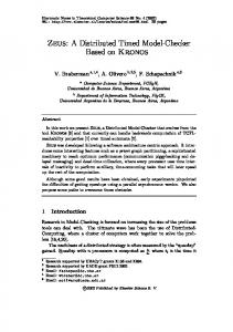
PK IND is implemented in OCaml and is built with components from (the sequential) K IND model checker [7] and the K IND-I NV invariant generator [9] we developed in previous work. Its concurrent components are implemented as operating system processes since OCaml’s concurrency model does not take advantage of multi-processor hardware to parallelize thread-level computation. We used the M PI (Message Passing Interface) API [11] to implement communication among the different processes. Figure 1 illustrates the general architecture of PK IND. For simplicity, we consider only the case of one invariant generation process. The extension to an arbitrary number of invariant generators (of the same type) is straightforward. Each process uses its own copy of the SMT-solver; and each of them receives as input the formulas encoding the Lustre program to be checked. The three processes, described below, cooperate as in the Actor model, exchanging messages asynchronously by means of non-blocking send and receive operations on message queues. Base process: Starting from k = 0, the base process checks the entailment of case (1) in the k-induction definition, for increasing values of k. If the entailment fails, it produces a counterexample and sends a termination signal M2 to the inductive step process. Otherwise, it keeps increasing k and checking the entailment until it receives a message M1 from the inductive step process stating that the process has proven the inductive step (2) for a certain value n of k. At that point, the base case process checks that the base case holds for that value of k, succeeding if it does and returning a counterexample otherwise. 1 Further improvements involve the addition of path compression constraints and checks [12, 10], which not only speed up computation but also guarantee completeness in certain cases—including all finite state systems.
T. Kahsai & C. Tinelli
57
Figure 1: PK IND general architecture. Inductive step process: This process checks the inductive step entailment for increasing values of k until one of the following occurs, in this order: (i) the entailment succeeds, (ii) it receives a termination signal from the base case process, or (iii) it receives an invariant from the invariant generation process. In the latter case, the inductive step process asserts the discovered invariant for all the states involved so far (from 0 to k + 1) before repeating the process with the same value of k. The inductive step process has an auxiliary role in this architecture—it is the base case process that determines whether the property is k-inductive or not. Invariant generation process: This process is composed of three modules. The Candidate generator, synthesizes a set of candidate invariant from predefined templates. The Int and Bool Invariants modules generate integer and Boolean type invariants respectively. Invariants are sent to the inductive step process, in messages M3 , as soon as they are discovered. The process keeps sending newly discovered invariants until it processes all candidates or it receives a termination signal M4 from the base process. This process produces k-inductive invariants for a given transition system S from a template R[ , ], a formula of L representing a decidable binary relation over one of system’s data types. The invariants are conjunctions of instances R[s,t] of the template produced with terms s,t from a set U of terms over the state variables of S . The set U can be determined heuristically from S (and possibly also from the property P to be proven) in any number of ways.2
2.1
Invariant Generation
The general invariant generation scheme introduced in [9] is illustrated in Figure 2, Version A. The twophase procedure, also based on k-induction, starts with a conjunction C of candidate invariants and first eliminates from C as many conjuncts as possible that have an actual counterexample. Then it attempts to prove the resulting C k-inductive, pruning any unprovable conjunct until it succeeds—possibly with an empty C in the worst case. All conjuncts of C that remain at the end are invariant and can be returned. Note that in Phase 1 the search for counterexamples stops when, for some k, C is falsified by no kreachable states. This is just a heuristic termination condition which does not preclude the possibility that some conjuncts of C may be falsified by longer counterexamples. As a consequence, every conjunct of C that does not pass the test in Phase 2 are conservatively assumed not to be invariant (even if it may be k0 -inductive for some k0 > k) and removed. 2 In our experiments, we constructed U with terms occurring in the L -encoding of S plus a few distinguished constants from the domain of S ’s variables.
58
PKind
proc invariant generator ≡ V C = s,t∈U R[s,t] k = −1 resetbase ; resetind // Phase 1 repeat k = k+1 assertbase (Tk ) changed = false while ¬ entailedbase (Ck ) do cex = project(cexbase ,Ck ) C = filter(C, cex) changed = true until ¬ changed // Phase 2 assertind (T1 ∧C0 ∧ · · · ∧ Tk+1 ∧Ck ) while ¬ entailedind (Ck+1 ) do cex = project(cexind ,Ck+1 ) C = filter(C, cex) send(D, ind proc) Version A (non-incremental)
generator ≡ proc invariant V C = s,t∈U R[s,t] k = −1 resetbase repeat k = k+1 assertbase (Tk ) while ¬ entailedbase (Ck ) do cex = project(cexbase ,Ck ) C = filter(C, cex) D=C resetind assertind (T1 ∧ D0 ∧ · · · ∧ Tk+1 ∧ Dk ) changed = false while ¬ entailedind (Dk+1 ) do cex = project(cexind , Dk+1 ) D = filter(D, cex) changed := true send(D, ind proc) until ¬ changed Version B (incremental)
Figure 2: General scheme for invariant generation. The procedures reset and assert and the functions entailed and cex, are all indexed by the copy of the L -solver used by the process. reset empties the solver’s set of asserted formulas; assert(F) adds the formula F to that set; entailed(F) returns true iff the currently asserted formulas L -entail F. When invoked after a call to entailed that returned false, cex returns a counterexample for that failed entailment. The function project takes an assignment α for state variables and a formula F, and returns the restriction of α to the variables of F. The function filter takes a conjunctive property P and an assignment α for P’s variables, and returns the property obtained from P by removing all conjuncts falsified by α. In Version B, D is meant to be a copy of C, not a renaming. The call send(D, ind proc) sends D to the inductive step process. The general invariant discovery scheme above produces a single conjunctive invariant at the very end. In a concurrent setting, however, it is better for runtime performance to have an incremental invariant generation process, which identifies and returns invariants as it goes. Concretely, it is better for the invariant generation process of PK IND first to identify, and immediately send to the inductive step process, conjuncts of C that are 0-inductive, then identify and send those that are 1-inductive, and so on. Pseudo-code for the incremental procedure is provided in Figure 2, Version B. The procedure starts V again with the conjecture C = s,t∈U R[s,t]. However, it does the following for every k ≥ 0. First, it eliminates from C all conjuncts falsified by a k-reachable state. Then it makes a copy D of C and tries to prove it k-inductive by checking the k-induction step on D. Counterexamples in that step are used to weaken D further, eliminating more and more conjuncts from it until no counterexamples exists. The final formula D is k-inductive and can be already sent to the inductive step process. If D did not need to be weakened at all, it means that all the conjuncts left in C after the base case check were k-inductive. Hence, the whole process terminates. If D was weakened, the eliminated conjuncts are either falsified by a longer counterexample or possibly k-inductive for a larger k. Those conjuncts are still in C, so in that case the procedure increases k by 1 and repeats with the larger k.
T. Kahsai & C. Tinelli
59
We point out that the conjuncts left in D (and sent out because k-inductive) are not removed from C before repeating. This is for simplicity but also for convenience because on the new iteration they will end up be in D again, strengthening the induction hypothesis for the inductive step check. That means, however, that the set of conjuncts sent out at iteration k + 1 is a (strict) superset of the one sent out at iteration k. This can be remedied by keeping the previous D and sending out only the difference between the new D and the old.3
2.2
Additional Features
PK IND takes full advantage of all the sophisticated features of its two embedded SMT solvers, such as their being on-line, incremental, backtrackable, and able to compute and return satisfying assignements or unsatisfiable cores of input formulas. It provides three different running modes: in k induct mode, PK IND functions as a basic parallel k-induction model checker, scheduling only the processes for the base and the inductive step; in no inc invariant mode, it creates also the invariant generation process. The invariant generation implemented here is Version A of Figure 2; in inc invariant mode, the invariant generation is done in an incremental fashion, as in Version B of Figure 2. PK IND includes a number of optional enhancements on top of this basic procedure, inherited from the K IND checker. The main ones are: path compression, termination checking and abstraction. Path compression strengthens the induction hypothesis with a formula that, in essence, removes from consideration program executions with repeated states or more than one initial state. Termination checking allows it to prove a non-k-inductive property in some cases by realizing that the reachable state space has been completely explored. Abstraction generates a structural abstraction of the idealized Lustre program and performs something similar to a CEGAR loop in both the base case and the induction step, with the goal of improving the tool’s scalability. See [7] for more information on these and other minor enhancements.
3
Experimental evaluation
We have evaluated PK IND and its different working modes experimentally against K IND and K IND-I NV using the same benchmark set as in [9].4 That set collects a variety of benchmarks from several sources, with each benchmark consisting of a Lustre program and a property to be checked for invariance. Let us call a benchmark valid if its property holds in every reachable state of the associated program, and invalid otherwise. K IND is able to show 438 of the 941 benchmarks in our set invalid by returning a (separately verified) counter-example trace for the program. K IND reports 309 of the remaining benchmarks as valid and diverges on the remaining 194 benchmarks, even with very large timeout values. For the experiments described here the benchmark set is divided in two groups: the 503 valid or unsolved benchmarks, and the 438 invalid ones. Our tests compare PK IND vs. K IND along two dimensions: precision, measured as the percentage of solved benchmarks, and runtime. For the latter, we were interested specifically in evaluating how the parallel architecture speeds up k-induction in the case of invalid benchmarks, and how incremental invariant generation contributes in decreasing solving times for valid benchmarks. The experiments were run on a 6-core 2.67 GHz Intel Xeon machine, with 6 GB of physical memory, under RedHat Enterprise Linux 4.0. Version 1.0.9 of the Yices solver was used both for PK IND and K IND. 3
In our experimental evaluation, however, this enhancement did not seem necessary because in most cases the first few sets of invariants were enough for the process ind proc to prove the input property. 4 Tools and experimental data can be found at http://clc.cs.uiowa.edu/Kind.
60
PKind
Figure 3: A comparison of generating counter-examples between PK IND -k induct and K IND on invalid benchmarks. On the left-hand side we compare PK IND -k induct and K IND in BMC mode. On the right-hand side we compare PK IND -k induct and K IND in inductive mode.
3.1
Precision results
As in [9], we used K IND-I NV to generate invariants offline. We first ran K IND-I NV on the benchmark set for 200 seconds. For each of the benchmarks where K IND-I NV did not time out, we obtained a set of invariants, and added them to the program as a single conjunctive assertion. The asserted formula was the constant true when K IND-I NV timed out or ended up discarding all conjectures from the initial set. Then, we ran K IND in inductive mode with a 100s timeout on each invariant-enhanced benchmark. K IND’s precision over the 503 valid or unsolved benchmarks grows from 61%, without invariants, to 85%, with the added invariants. For each additional benchmark proved valid, the property goes from (most likely) not k-inductive for any k to k-inductive for k ≤ 16. Using the same time out value, in k induct mode PK IND proves valid the same benchmarks proven by K IND with no invariants. In either no inc invariant and inc invariant mode, PK IND proves the same benchmarks proven by K IND with invariants, despite the fact that it generates invariants on the fly, whereas K IND gets them as input.5 Precision is also unchanged when comparing PK IND with K IND run (in a much faster) BMC mode on the set of 438 invalid benchmarks. Furthermore, in all these cases, solving times are shortened considerably with PK IND, as discussed below.
3.2
Runtime results
The two scatter plots in Figure 3 compare the runtimes of PK IND -k induct with those of K IND respectively in BMC mode (left-hand side plot), which performs just bounded model checking, and inductive mode (right-hand side plot), which performs full k-induction. The timeout for both tools was 200s. As the first plot clearly shows, the runtimes of the two tools are pretty much the same in the first case. Due to some overhead of the M PI implementation in PK IND, for some benchmarks K IND is slight faster. The average solving time for PK IND -k induct is 2.34s, while for K IND in BMC mode it is 2.29s. The superiority of PK IND is clearly illustrated with the second plot. For a more quantitative comparison, both tools are able to produce a counterexample in less than 1s per benchmark for 90% of all invalid benchmarks. However, PK IND -k induct takes less than 82s to solve any of the invalid benchmarks, whereas K IND in inductive mode times out on half of them. It is worth stressing that PK IND -k induct is also superior from a usability perspective because it combines the speed of K IND’s BMC mode over invalid inputs with the generality and precision of K IND’s inductive mode, without requiring the user to chose between these two modes. 5 As a precaution against implementation errors, each invariant produced by K IND -I NV or by PK IND was independently and successfully verified by giving it to K IND separately as a property to prove for the program from which it was generated.
T. Kahsai & C. Tinelli
61
Figure 4: A comparison of solving the benchmarks between PK IND -no inc invariant and PK IND inc invariant on valid benchmarks. On the left-hand side we compare the two modes on benchmarks which are valid without the addition of invariants. On the right-hand side we compare the two tools on the benchmarks previously unsolved. Both plots use a log-log scale over seconds. Moving to PK IND’s invariant generating modes, since invariants for K IND are generated offline, it is not possible to do direct runtime comparisons between the two systems over the valid or unsolved benchmarks. A more interesting comparison is between the two invariant generating modes themselves. In a nutshell, our results show that the addition of incrementally produced invariants, makes those benchmarks considerably faster to solve. In more detail, we first compared PK IND -no inc invariant and PK IND -inc invariant on all previously valid benchmarks, those that can be shown valid without the addition of invariants. On those benchmarks, the conjunctive invariant produced by the non-incremental version has no effect on the k-induction loop, because the property is invariably proven before the invariant is generated. In contrast, when invariants are generated incrementally, they are in many cases sent to the inductive step process early enough to play a role in reducing the overall solving time. The left-hand side of Figure 4 provides a comparison between the two invariant generation modes. The plot demonstrates how incremental invariant generation speeds up runtimes. Specifically, the incremental version is able to solve 76% of all the valid benchmarks in less than 0.02 seconds, while the non-incremental version can do that for only 17% of those benchmarks. Looking at the previously unsolved benchmarks, with a timeout of 100s, both invariant generation modes solve 66% of them. Again, however, the incremental version is faster than the non-incremental one although the speed up is less pronounced, as can be seen in the right-hand side plot of Figure 4. In more detail, the incremental version is able to solve 79% of all newly solved benchmarks in less than 9s, whereas the non-incremental version is able to solve 73% of them. It is interesting to observe that in a few cases non-incremental invariant generation is slight faster than the incremental one. The reason for this is that the useful invariant is one that is k-inductive for a relatively larger k than usual.6 In those cases, incrementally sending and processing (useless) k-inductive invariants for lower values of k produces a bit of overhead. With regard to the size of our benchmarks, the invalid ones range from 200 bytes to 40KB of Lustre source code with no comments and standard use of white space. The average time to solve an invalid benchmark of size more than 20KB is 9.12 seconds. For the valid benchmarks the size ranges from 400 bytes to 58KB. The average time to solve a valid benchmark of size more than 20KB bytes is 17.6 seconds. Although benchmark sizes may appear small, we stress that the majority of these benchmarks are infinite-state systems written in a high level specification language, so a benchmark’s size is not a 6
In most benchmarks in our set, adding 0- or 1-inductive invariants is enough to make the property provable.
62
PKind
good predictor of its difficulty. In fact, looking at runtime data over the whole benchmark set we found no correlation between benchmark size and solving times.
4
Conclusion and future work
We have described PK IND, a novel parallel k-induction-based model checker. PK IND is designed to keep interprocess synchronization overheads to a minimum and easily accommodate the concurrent automatic generation of invariants to bolster the basic k-induction procedure. While any independent invariant generation techniques could be used in principle in our architecture, we have developed a new one, based on our previous work, that produces invariants in an incremental fashion to exploit the advantages of the parallel setting. Our experimental results provide an initial and clear evidence that the architecture significantly speeds up the verification of safety properties. In addition, due to the incremental invariant generation, this architecture considerably increases the number of provable benchmarks. In future work, we plan to study new ways of automatically generating invariants for k-induction, both in parallel, i.e., using abstract interpretation techniques, and on-demand, in response to counterexamples found by the inductive step. We are also working on a new version of PK IND built from scratch around the architecture discussed here and designed to accept other input languages besides Lustre.
References ´ [1] Erika Abrah´ am, Tobias Schubert, Bernd Becker, Martin Fr¨anzle & Christian Herde (2011): Parallel SAT solving in bounded model checking 21(1), pp. 5–21, doi:10.1093/logcom/exp002. ˇ ska & P. Roˇckai (2010): DiVinE: Parallel Distributed Model Checker (Tool paper). [2] J. Barnat, L. Brim, M. Ceˇ In: HiBi/PDMC 2010, IEEE, doi:10.1109/PDMC-HiBi.2010.9. [3] Clark Barrett & Cesare Tinelli (2007): CVC3. In W. Damm & H. Hermanns, editors: CAV’07, LNCS, Springer, doi:10.1007/978-3-540-73368-3 34. [4] Aaron R. Bradley (2011): SAT-based model checking without unrolling. VMCAI ’11, Springer-Verlag, pp. 70–87. Available at http://dl.acm.org/citation.cfm?id=1946284.1946291. [5] Bruno Dutertre & Leonardo de Moura (2006): The YICES SMT Solver. Technical Report, SRI International. Available at http://yices.csl.sri.com/. [6] Niklas E´en & Niklas S¨orensson (2003): Temporal induction by incremental SAT solving. Electr. Notes Theor. Comput. Sci. 89(4), doi:10.1016/S1571-0661(05)82542-3. [7] George Hagen & Cesare Tinelli (2008): Scaling up the formal verification of Lustre programs with SMTbased techniques. In: FMCAD ’08, Piscataway, NJ, USA, pp. 1–9, doi:10.1109/FMCAD.2008.ECP.19. [8] N. Halbwachs, P. Caspi, P. Raymond & D. Pilaud (1991): The synchronous data-flow programming language Lustre. Proceedings of the IEEE 79(9), pp. 1305–1320, doi:10.1109/5.97300. [9] Temesghen Kahsai, Yeting Ge & Cesare Tinelli (2011): Instantiation-Based Invariant Discovery. In: NFM 2011, LNCS 6617, Springer, pp. 192–207. Available at http://dl.acm.org/citation.cfm?id= 1986308.1986326. [10] Leonardo de Moura, Harald Rueß & Maria Sorea (2003): Bounded Model Checking and Induction: From Refutation to Verification. In: CAV 2003, LNCS 2725, Springer, doi:10.1007/978-3-540-70952-7 21. [11] Peter S. Pacheco (1997): Parallel programming with MPI. Morgan Kaufmann Publishers Inc. [12] Mary Sheeran, Satnam Singh & Gunnar St˚almarck (2000): Checking Safety Properties Using Induction and a SAT-Solver. In: FMCAD ’00, Springer-Verlag, London, UK, pp. 108–125, doi:10.1007/3-540-40922-X 8. [13] Siert Wieringa, Matti Niemenmaa & Keijo Heljanko (2009): Tarmo: A Framework for Parallelized Bounded Model Checking. In: PDMC ’09, pp. 62–76, doi:10.4204/EPTCS.14.5.