Cointegration Tests Using Instrumental Variables Estimation and the Demand for Money in England Kyung So Im
Junsoo Lee
Walter Enders
June 12, 2005
Abstract In this paper, we propose new cointegration tests based on stationary instrumental variables in a single equation model. An important property of our tests is that the asymptotic distribution is standard normal. As such, our IV cointegration tests provide a convenient solution to the nuisance parameter dependency problem found in existing cointegration tests. In addition, the asymptotic distribution of the IV tests does not depend on the dimension of the regressors or di¤ering deterministic terms. We apply the new IV tests to estimate the demand for money equation for England.
JEL Classi…cation: C12, C15, C22 Key Words: Cointegration Test, Stationary Instrumental Variables, Standard Normal Distribution Kyung so Im is Associate Professor, Department of Economics, University of Central Florida, Orlando, FL 32816 (email:
[email protected]); Junsoo Lee (Corresponding author) is Associate Professor, Department of Economics, Finance and Legal Studies, University of Alabama, Box 870224, AL 35487 (email:
[email protected], phone: 205-348-8978, fax: 205-348-0590); and Walter Enders is Professor and Lee Bidgood Chair of Economics and Finance, Department of Economics, Finance and Legal Studies, University of Alabama, Tuscaloosa, AL 35487 (email:
[email protected]).
1
1
Introduction
The pioneering work by Engle and Granger (1987, EG hereafter) addresses the issue of testing if non-stationary time series are cointegrated. It is well known that the limiting distribution of the EG cointegration test is nonstandard. The distribution depends on the number of regressors as well as the form of the deterministic terms. Thus, one needs to use di¤erent critical values for di¤erent speci…cations of the model. Various extensions of the EG test have been suggested and the distributions of these cointegration tests are also nonstandard. In this paper, we propose new cointegration tests based on stationary instrumental variable (IV) estimation in a single equation framework. One important feature of our stationary IV cointegration tests is that their asymptotic distributions are standard normal. As such, the limiting distributions of the IV tests do not depend on the dimension of the regressors or on the deterministic terms. This is a convenient result. Regardless of various model speci…cations, one can use the same asymptotic critical value of 1:645 at the 5% signi…cance level. This feature cannot be found in existing cointegration tests based on OLS estimation. More importantly, the asymptotic normality result for the IV cointegration tests implies that we can provide a solution to the problem of nuisance parameter dependency when testing for cointegration. Speci…cally, the present paper seeks to resolve the following problems of existing cointegration tests. First, our IV cointegration approach provides a solution to the nuisance parameter problem present in other cointegration tests based on error correction models (ECMs). Many authors have noted that the asymptotic distribution of the ECM based cointegration test statistic depends on a nuisance parameter when it is a mixture of two quite di¤erent distributions, viz, the Dickey-Fuller (DF) type nonstandard distribution and the standard normal distribution. The nuisance parameter describes the relative importance of each of these distributions; see Boswijk (1994) among others. The nuisance parameter is unknown and can take any unknown value. This dependency problem has hindered researchers from applying the ECM cointegration test. However, when the IV estimation is applied to the ECM the distribution of the resulting t-statistic is standard normal. Second, by utilizing IV estimation in the EG type procedure, the IV cointegration test also provides a solution to the common factor restriction problem imposed in the EG test. One well known problem is that the EG 2
procedure imposes a strict dynamic restriction which may not hold. Although the coe¢ cients in the cointegration relationship usually di¤er from the short run adjustment coe¢ cients, the two sets of coe¢ cients are assumed to be equivalent in the EG procedure. Kremers, Ericsson and Dolado (1992) refer to this restriction as a common factor restriction (CFR). Another problem that results from imposing the CFR is that the test loses power when the signal-noise ratio increases. Although it is possible to resolve this problem by adding the di¤erenced regressors, the result is to generate the same problems as in the ECM based test. Our IV cointegration tests are free of this type of problem as the testing regression does not impose a common factor restriction. Moreover, our IV test gains power when the signal-noise ratio increases, although the OLS based EG test loses power when the signal-noise ratio increases. The reason for increased power is quite intuitive; the added regressors enter as stationary covariates in our testing regressions. As shown by Hansen (1995), the use of stationary covariates can enhance the power of unit root tests. A similar advantage can be obtained in the IV cointegration tests. The di¤erence is that the distribution of the IV cointegration tests still remain as standard normal and is free of the nuisance parameter problem. Finally, the IV tests can be adopted in an autoregressive distributed lag (ADL) model. The ADL test also requires weak exogeneity of the regressors; see Banerjee, Dolado and Mestre (1998). Under this condition, the ADL model yields e¢ cient estimates of the parameters in the model. The ADL test is free of the CFR and its null distribution does not depend on the signal-noise ratio. However, the ADL test depends on nuisance parameters that enter the deterministic components of the data. Thus, the ADL tests depend on the number of regressors and other deterministic components. In contrast, the asymptotic distribution of the IV cointegration tests remain as standard normal, regardless of di¤ering deterministic terms or the number of regressors. The remainder of the paper is organized as follows. In Section 2, we illustrate the major testing models and examine their relationships. In Section 3, we consider the stationary IV cointegration tests in the error correction model and the EG procedure. We provide relevant asymptotic results. In Section 4, we examine the …nite sample performance of the tests. Section 5 provides concluding remarks.
3
2
Single Equation Cointegration Models
As Ericsson and MacKinnon (2002) explain, there have been three main approaches to testing for cointegration: a system based full information maximum likelihood estimation of a vector error correction model as developed by Johansen (1989), a two step procedure based on a single-equation regression suggested by Engle and Granger (1987), and a single-equation conditional error correction model suggested by Banerjee et al. (1986). Ericsson and MacKinnon discuss the advantages and disadvantages of each of these approaches. Perhaps, the Johansen procedure has been the most popular in applied work since it provides the most e¢ cient estimates of the parameters in the model. Ericsson and MacKinnon point out that Johansen’s test requires a well-speci…ed full information system and that there are circumstances in which testing for cointegration can be performed properly in a single equation model under certain conditions. Zivot (2000) discusses various examples for which economic theory can imply a single cointegrating vector and explains why it is reasonable to test for cointegration in single equation models in such cases. In this paper, we also deal with single equation cointegration models. To begin with, we consider a VAR(p) model yt = dt + xt ;
(1)
(L)xt = "t ;
(2)
where yt , t = 1; 2; :::; T; is a n 1 vector of I(1) process, dt denotes deterministic terms, and xt is the stochastic component following an autoregressive Pp 1 i process with (L) = I i L and "t s iid; N (0; ). The normality i=1 assumption of the error term is made for convenience, but this assumption is not required for the asymptotic results. One can consider the deterministic term with dt = c1 for the model with a constant, or dt = c1 + c2 t for a model with a trend, but one may also allow for additional polynomial trends and dummy variables to capture seasonality or structural change. It is convenient to write (1) and (2) as a vector error correction model yt = c11 + c2 t + Here, we let
=
0
yt
(1) and express =
0
1
+ (L) yt
1
+ "t :
in a cointegrated system as 1
=
2
4
(1;
0
);
(3)
where 1 is a scalar and 2 and are (n 1) 1 vectors. We can express the conditional equation of y1t given y2t and other past values of yt , and the corresponding marginal equation of y2t as follows y1t = (d11 +d12 t)+ y2t =
0
1:2 (y1;t 1 0
2 (yt 1
y2;t 1 )+
y2;t 1 ) +
21
0
0 y2t +C11 y1;t 1 +C12 y2;t 1 +"1:2t ; (4) 0 y1;t 1 + 22 y2;t 1 + "2t ; (5)
where "1:2t = "1t 0 "2t such that E("1:2t "2t ) = 0: Many authors suggest that if y2t is weakly exogenous for the parameters 1 and ; then these parameters can be e¢ ciently estimated in the conditional error correction model (4). The weak exogeneity of y2t implies that 2 = 0, so that y2t is not errorcorrecting. In this case, we obtain that 1:2 = 1 ; see Harbo et al. (1998). Under this assumption, the parameters of interest can be e¢ ciently estimated in the conditional error correction model (4) without having to refer to (5) together. Then, we can rewrite (4) as y1t = (d11 + d12 t) +
1 zt 1
+
0
y2t + C11 y1;t
1
0 y2;t + C12
1
+ vt ; (6)
0 with zt 1 = y1;t 1 y2;t 1 and one can test the null hypothesis of no cointegration against the alternative hypothesis of cointegration
H0 :
1
= 0;
against H1 :
1
< 0:
To test this hypothesis, we use the usual t-statistic. This is the ECM based cointegration test for which the cointegrating vector is assumed to be prespeci…ed; see Banerjee et al. (1986), Kremers et al. (1992), and Zivot (2000), among others. On the other hand, the conditional ECM can be reparameterized as the conditional autoregressive distributed lag (ADL) model y1t = (d11 +d12 t)+ 1 y1;t
1+
0
y2;t
1+
0
y2t +C11 y1;t
0 1 +C12
y2;t
1 +vt :
(7) We can relate the above equation to (6) with 1 0 = 0 : It is clear that 1 = 0 implies = 0 as well, but 1 is una¤ected by an arbitrary value of ; say, = 1 0 where is an arbitrary long-run coe¢ cient. Thus, the null of no cointegration can be tested on 1 = 0 against H1 : 1 < 0 in (7). The resulting t-statistic from (7) is another version of the ECM version cointegration, but it is obtained from the unrestricted ADL model. Banerjee et al. (1998) adopt this test and provide critical values for the models with a constant and trend with the number of regressors up to 5. 5
The Engle and Granger cointegration test is based cedure. In the …rst step, the OLS estimate of ; say regression of y1t on y2t . Then, the EG cointegration t-statistic on 1 = 0 in the regression, ( y1t
^ 0 y2t ) =
on the two step pro^ ; is obtained in the test is based on the
^ 0 y2;t 1 ) + C(L)( y1t
1 (y1;t 1
^ 0 y2t ) + ut :
(8)
Obviously, the same value of ^ is used in both sides of the equation. This implies that the short-run coe¢ cient in the regression of y1t on y2t is assumed to be equivalent to the long-run coe¢ cient in the regression of y1t on y2t : To see this in more detail, we suppress the deterministic terms and the lagged terms of y1t and y2t in (6) and relate it to (8) as y1t
0
y2t =
0
1 (y1;t 1
y2;t 1 ) + (
0
0
) y2t + et :
(9)
We rewrite this as zt =
+ et ;
(10)
) y2t + et :
(11)
1 zt 1
where et = (
0
0
It is clear that the restriction = is imposed in the EG procedure. This restriction is referred to as the common factor restriction which may or may not hold. When the common factor restriction does not hold, the EG test can lose power; see Kremers et al. (1992). Note that the EG test does not require the weak exogeneity assumption, which is necessary for the ECM based test. In addition, we note that the asymptotic distributions of both ECM and EG type cointegration tests depend on the dimension of integrated regressors and di¤ering deterministic terms. The ECM and ADL type tests are free of the CFR problem, but they depend on the dimension of regressors and deterministic terms. In estimating 1 in each of (6) and (8), OLS estimation has been adopted in the literature. The limiting distribution of the resulting t-statistic based on OLS estimation is already provided; see Kremers et al. (1992) and Boswijk (1994) for the ECM cointegration test, Banerjee et al. (1998) for the ADL cointegration, and Engle and Granger (1987) and Phillips and Ouliaris (1990) for the EG type cointegration test. As noted previously, it is known that the asymptotic distribution of the t-statistic based on the ECM is a mixture of the DF type non-standard distribution and a standard normal distribution. Furthermore, it depends on the nuisance parameter which describes 6
the relative importance of each of these distributions; see Boswijk (1994) and Zivot (2000). The nuisance parameter is unknown, and this dependency has been a source of the problem that hinders from using the ECM cointegration test. The asymptotic distribution of the EG cointegration test is also nonstandard, having a Dickey-Fuller type distribution. The EG test is free of the nuisance parameter problem, but it loses power when the signal-noise ratio increases. In the next section, we demonstrate how the IV cointegration tests provide solutions to these problems of the OLS based cointegration tests.
3
Stationary IV Cointegration Tests
In this paper, we consider instrumental variables (IV) estimation of 1 in each of (6), (7) and (8). Speci…cally, we de…ne the instrumental variable, wt , di¤erently for each model, as wt = zt 1 zt m 1 ; for zt 1 in (6) 0 0 wt = (w1t ; w2t ); for (y1;t 1 ; y2;t 1 ) in (7) wt = z^t 1 z^t m 1 ; for z^t 1 in (8);
(12)
0 = where m T is a …nite positive integer, w1t = y1;t 1 y1;t m 1 ; and w2t 0 0 ^ y2;t 1 for which is estimated from y2;t 1 y2;t m 1 . Here, z^t 1 = y1;t 1 the regression of y1t on y2t as
y1t = (d11 + d12 t) +
0
y2t + error:
(13)
In a more general case where the error terms are serially correlated, the instrumental variable needs to be adjusted by subtracting more lags. For instance, wt is modi…ed as wt = zt 1 zt 1 p m for the ECM model. For each of the regressions in (6), (7), and (13), a constant term (d11 ), or both the constant and a trend function (d11 + d12 t) can be included. The t-statistic on 1 = 0 using the IV estimation with the corresponding instrumental variables wt is our suggested test statistic for cointegration in each of three models ti =
^1;IV
i
s(^1;IV i )
,
i = ECM, ADL, and EG.
(14)
Then, we refer to each of the corresponding t-statistics as tECM ; tADL ; and tEG , respectively. The distribution of these statistics is shown to follow a 7
standard normal distribution. To see this in more detail, we suppress the deterministic terms for simplicity and rewrite each of the testing regressions. For example, in considering the ECM test, we express the conditional ECM model in (6) as y1t = 1 zt 1 + 0 qt + vt ; (15) 0 0 0 0 where qt = ( y1;t 1 ; ::; y1;t p+1 ; y2t ; y2;t = (c11;1 ; ::; 1 ; ::; y2;t p+1 ) and 0 0 0 0 c11;p 1 ; ; c21;1 ; ::; c21;p 1 ) . In practice, when the cointegrating vector is unknown, the term zt 1 in (15) is not feasible. In that case, we replace zt 1 in (15) with z^t 1 and construct the IV as wt = z^t 1 z^t m 1 ; for z^t 1 . Then it can be shown that
tECM
T P
wt y1t t=1 s = T P wt2 ^ t=1
where
T 1X ^ = T t=1 2
T P
t=1
wt qt0
T P
wt qt0
t=1
T P
t=1
qt qt0
T P
^1;ECM z^t
y1t
qt qt0
t=1
1 T P
qt y1t
t=1
1 T P
;
(16)
qt wt
t=1
1
^ 0 qt
2
:
The asymptotic distribution of tECM is given as follows. Theorem 1 Suppose that yt is generated as an independent vector time series as in (1) , and the t-statistic in (14) is obtained by (16). Then as T ! 1, d
tECM ! N (0; 1):
(17)
Proof. See the Appendix. Since the asymptotic distribution of tECM is standard normal, it is clear that the distribution does not depend on any nuisance parameters. In addition, the asymptotic distribution of the IV statistics is una¤ected by the dimension of the regressors (y2t ) or the deterministic terms. It is also standard normal when a constant or trend function is allowed in the testing regression. This …nding can be extended when dummy variables accounting for structural change are added or when a polynomial time trend is included. The distribution remains as standard normal. Intuitively speaking, this is so because the second term in each of the numerator and denominator in 8
(16) disappear asymptotically. They remain as Op (T 1=2 ) or Op (T 1 ) when additional deterministic terms or stationary terms are included in qt . In addition, asymptotic normality of the test statistic holds as augmented terms are added. If potentially non-stationary terms are added, we need to instrument them to obtain the normality result. This is the case with the ADL based test. The normality result follows since the remaining …rst term in each of the numerator and denominator is expressed by stationary terms. That is, wt in (12) is stationary by construction under both the null of no cointegration and the alternative hypothesis. The same normality results are expected to hold for tADL and tEG owing to the same reasoning. Corollary Suppose that y t is generated as an independent vector time series as in (1) , and the t-statistics tADL and tEG are obtained as in (14). Then as T ! 1 d
d
tADL ! N (0; 1) and tEG ! N (0; 1):
(18)
The property of the IV cointegration test makes a sharp contrast with the OLS based test statistic whose distribution is a mixture of the DF type nonstandard distribution and a standard normal distribution, implying that the OLS based statistic depends on a nuisance parameter indicating the relative contributions of the two di¤erent distributions. It is well know that the OLS based statistic also depends on the deterministic terms and dimension of stochastic terms describing the non-standard distribution. We note that the coe¢ cient estimates, ^1;i ; i = ECM; ADL or EG, do not follow a normal distribution. Their distribution is a mixture of a nonstandard and standard normal distribution. It has similar properties to those of the OLS based statistics p shown in Zivot (2000) and Hansen (1995). One di¤erence is that ^1;i is a T -consistent estimator, instead of a T -consistent estimator. Note that the instrument wt is asymptotically uncorrelated with the instrumented variable under the null hypothesis of no cointegration. Howm ever, under the alternative hypothesis, their correlation coe¢ cient is 1 1 ; which essentially implies consistency of the test under the alternative. These are asymptotic results in large samples and may not hold in …nite samples. When additional deterministic terms are added or the dimension of the regressors increases, a slower convergence rate can be observed in …nite samples. In this case, the issue of choosing proper lags and valid instrumental variables arises. However, this outcome occurs mostly in small samples as the sample size increases, the bias term disappears. It is important to note 9
that our result holds asymptotically with proper values of m; which increases as T increases. In …nite samples, the terms that disappear asymptotically remain as bias terms. As such, although the asymptotic result is rather straightforward for a …nite value of m, the size property of the test in …nite samples depends on the selected value of m. At the same time, a moderately big value of m is necessary for obtaining desirable power properties. No immediate theoretical guidance is readily available in selecting the optimal value of m. Some practical guidance on the choice of m can be found for di¤erent values of T from the simulation results in Table 1. For the EG type IV test, we modify (8) and suggest augmenting y2t . As discussed in Kremers et al. (1992), we lose potentially valuable information from y2t by omitting it in the EG testing regression. Adding y2t amounts to not imposing the common factor restriction. As we see in (11), by adding y2t in the testing regression, we do not necessarily impose the restriction that = . Thus, we have z^t =
^t 1 1z
+
0
y2t + ut ;
(19)
where z^t is the residual from the regression in (13). We refer to the resulting t-statistic for 1 = 0 as t+ y2t in the usual EG EG . Note that one cannot add test based on OLS estimation. When y2t is added, the distribution of the resulting test depends on the nuisance parameter, which is essentially the same problem of the OLS based ECM test.
4
Simulations
In this section, we investigate small sample properties of the IV cointegration tests through Monte Carlo simulations. We use di¤erent values of m = 1; ::; 9. We consider four IV statistics described in the previous section. They are tECM , tADL , tEG , and t+ EG . In addition, for comparison, we report the simulation results using the OLS based tests. They are denoted as tECM O , tADL O , and tEG O , where the subscript "o" was added to signify the use of OLS estimation. We simulated new critical values for the OLS based tests for each of di¤erent values of k, T and di¤erent models, and used them to compute the size and power of the tests. The simulated critical values are provided in the footnote of corresponding tables. On the other hand, for the IV tests, we use the asymptotic one-sided asymptotic critical value 1:645 of the standard normal distribution at the 5% signi…cance level for all cases. 10
We adopt the following data generating process (DGP) as in Kremers et al. (1992) y1t = 0 y2t + 1 (y1t y2t = ut 2 vt 0 v N ; ut 0 0
0
y2t ) + vt ;
0 2 u
(20)
:
All simulation results are based on 20,000 replications. We denote k as the number of integrated regressors, viz the row dimension of y2t . When 1 = 0, the DGP implies no cointegration. When 1 < 0, the DGP implies cointegration. We start with the case of k = 1, in which we examine the e¤ect of using di¤erent signal-noise ratios on the size and power. We set = 1: We denote s = u = v and de…ne the signal-noise ratio v = 1 and as q = ( 1)s. Then, we examine the cases with ( ; s) = (1.0, 1), (0.5, 6), and (0.5, 16) such that q = 0; 3, and 8. Following this, we examine whether the tests are sensitive to the number of integrated regressors with k = 3. When k = 3, we use the same set of values of ( ; s) for all integrated regressors. We examine two di¤erent models; one is the drift model with dt = c1 (the results are reported in Tables 1 - 4) and the other is the trend model with dt = c1 + c2 t (the results are reported in Tables 5 - 8). The instrumental variables are given in (12). A special attention will be given to robustness of the standard normal result of the IV tests under di¤erent model speci…cations and di¤erent values of q. For each model, we report the results with T = 100 and 300. We also examined the cases of T = 500 or 1; 000, but these results are not much di¤erent from the results of T = 300, except for more desirable results of increased power or such. In Table 1, we report the size of various tests under the null of no cointegration with k = 1 and 3; when we include a constant term in dt . The OLS based tests should have the correct size as customized critical values are used. It appears that all IV tests show more or less the correct size, which lies within a 1% error from the nominal 5% size, when a proper value of m is selected. One exception is that no values of m give the correct size for tEG : Also, it is apparent that the sizes of all IV tests are not changed much with k = 3 when compared to the case with k = 1. We observe that almost no changes are observed for tECM : This result indicates that the IV tests are invariant to k; the number of endogenous integrated variables in the model. More importantly, it is shown that the IV test tECM is invariant to the signalnoise ratio (q), although the corresponding OLS based test tECM O critically 11
depends on q. Thus, the IV test resolves the nuisance parameter dependency problem of the OLS based ECM test tECM O . All other IV tests also seem insensitive to di¤erent values of q under the null. For the OLS based tests, we can use customized critical values for a given model when they have non-standard distributions. For the IV tests, we wish to use only one asymptotic critical value, -1.645, for all di¤erent cases with di¤erent model speci…cations. To this end, we wish to select a correct value of m that gives a correct size under the null. However, no clear guidance is readily available regarding the selection of m. Theoretically speaking, any …nite value of m will lead to the asymptotic standard normal result, but this is not necessarily the case in …nite samples. The best values of m that lead to a correct size under the null vary over di¤erent models in …nite samples. Our simulation results may provide guidance in this regard. As such, to have a better sense of this matter, we underlined the values of m that give the closest size to the nominal 5% size for each case. In Figure 1, as an example, we illustrate the pdf of the empirical distribution of tECM using di¤erent values of q, k and m under the null hypothesis when T = 100. These empirical distributions are based on the kernel estimation using a Gaussian kernel function. The solid curve depicts the pdf of the standard normal distribution. We can observe that the pdfs of the IV statistics are close to the pdf of the standard normal distribution, regardless of the values of q. On the contrary, we observe in Figure 2 that pdfs of the t-statistics of the OLS based ECM test (tECM O ) vary signi…cantly over di¤ering values of q. As q increases, the pdf moves to the right away from the pdf with q = 0 (solid curve on the left). Thus, they show serious size distortion when q > 0. In Table 2, we examine the size adjusted power of the tests when 1 = 0:1: We observe that the IV ECM test tECM performs well. The tECM test is more powerful than other IV tests and is fairly comparable to the OLS based ADL tests. For instance, the power of tECM is 0:257 when m = 7, while the power of tADL O is 0:244. The OLS ECM test tECM O appears more powerful than any others but tECM O is not a valid test as examined in Table 1. Thus, we exclude this test from further discussion. In general, the ECM and ADL based tests are more powerful than the EG tests. Our interest lies in examining the e¤ect of q: The power of the EG tests (tEG and tEG O ) decreases as q increases. Under the null, these tests do not depend on the signal-noise ratio q, but they depend on q under the alternative. A similar result for the OLS based EG test was discussed in Kremers et al. (1992). 12
The source of this problem is that these tests omit the term y2t from the testing regression. However, the modi…ed EG test t+ EG is not subject to this problem when y2t is added as in (19). The power of the t+ EG test increases as the signal-noise ratio increases. As noted in the previous section, adding y2t in the EG procedure amounts to relaxing the common factor restriction (CFR). In the OLS framework, we cannot add y2t since it leads to the nuisance parameter problem and invalid tests. But, in the IV framework the null distribution remains as standard normal, implying absence of the nuisance parameter dependency problem, and the power increases under the alternative. The power of the ECM and ADL tests increases as q increases. This phenomenon is observed for both IV and OLS based tests (tECM , tADL , and tADL O ). Thus, in addition to the t+ EG test, both tECM and tADL also solve the problem of losing power in the usual EG tests when the signal-noise ratio increases. In Figure 3, we plot the pdf of the empirical distribution of the t-statistics for the IV test tECM by varying the values of the signal-noise ratio (q) under the alternative hypothesis when T = 100 and k = 1 or 3. We wish to illustrate graphically the e¤ect of using di¤erent values of q on the power of the test. It is clear that the pdfs of the IV statistic of tECM shifts leftward away from the pdf of the normal distribution, thereby gaining power as q increases. The underlying logic for increased power is similar in nature to the …nding of Hansen (1995) who showed that power of the usual unit root tests increases by adding stationary covariates. In our framework, y2t works the same as stationary covariates, and the gain in power is bigger when the variance of y2t gets bigger so that the signal-noise ratio increases. This e¤ect is enhanced as the dimension of y2t (k) increases with more regressors. Then, the power increases further as k increases. The far-left truncated curve shows the case when k = 3. This phenomenon is the opposite direction of the OLS based tests whose power decreases as k increases. In general, power normally decreases as k increases since additional parameters need to be estimated. In the IV tests, the e¤ect of increasing power with additional covariates is usually bigger than the e¤ect of decreasing power. If not, the test loses power. This occurs in the t+ EG test; it loses power as k increases. However, it is encouraging that the power of tECM is not reduced as k increases. Indeed, in some cases, the power of the tECM test increases; see the case in Table 2 when q = 3 as k increases from 1 to 3. We note that the IV version of the ADL test (tADL ) is less powerful than the OLS version of the ADL test (tADL O ): This result is expected since the OLS based tests 13
are usually more powerful. However, the tECM test is fairly comparable to tADL O : In Tables 3 and 4, we replicate the same simulations as in Tables 1 and 2, but only with a large sample size of T = 300: The properties of the tests are similar to those with T = 100, except that the power of the test increases as the sample size increases. It is clear that a higher value of m is needed for the IV tests to have a correct size under the null when the sample size increases. We underlined the values of m that give the size closest to the nominal 5% size for each case. In Tables 5 - 8, we report the results with the trend model. Note that the same asymptotic critical value of 1:645 is used in all cases for the IV tests. The outcome remains similar to that in the previous simulation results with only a constant and the basic results on the properties of the tests remain unchanged. We do not observe any signi…cant size distortion or signi…cant loss of power by adding the trend function. The power of all tests decreases somewhat, when compared with the drift model, but this result is expected when we deal with more general models. Again, we conclude that the standard normal result still holds in the trend model. Overall, the IV tests are reasonably robust to di¤erent model speci…cations. This is an expected outcome due to the fact that the IV cointegration tests do not depend critically on the usual deterministic terms. As noted, our tests do not critically depend on the number of integrated regressors. We expect that similar results will follow when structural breaks are allowed. Most important, the IV tests are invariant to the nuisance parameters that make the OLS based tests invalid. The IV cointegration tests do not depend on the signal-noise ratio under the null, and their power increases as the signal-noise ratio increases under the alternative.
5
Empirical Example: The Demand for Narrow Money in the U.K.
We now illustrate the appropriate use of our IV test using an extended example from the literature. To avoid the appearance of selecting an arbitrary set of variables, we use the data set complied by Hendry and Ericsson (1991) for their study of the demand for narrow money in the U.K during the 1964:Q3 ~ 1989:Q2 period. This data is widely available, has been studied intensively,
14
and has interesting time-series properties.1 For our purposes, the data is particularly appealing because it has been estimated and tested using the Johansen FIML procedure as well as the single equation-based procedures. For example, Hendry (1995) used the Johansen methodology to obtain the following estimates of possible cointegrating relationships among the variables of the money demand function 2 3 2 3 (m p)t 1:00 1:00 7:34 7:65 0:0005 6 7 it 6 0:06 1:00 76 7 3:38 0:86 0:0059 6 76 7; p (21) t 7 4 0:29 0:69 1:00 0:63 0:0025 5 6 4 5 Rt 0:03 1:58 1:10 1:00 0:0097 t
where mt = the log of nominal narrow money, it = the log of real total …nal expenditure (TFE) at 1985 prices, pt = the log of the TFE de‡ator, Rt = the di¤erence between the three-month local authority interest rate and a learning-adjusted retail sight-deposit interest rate, and t = time index. The max and trace statistics indicate exactly two cointegrating vectors among the four variables. A long-run money demand relationship can be identi…ed by imposing a unitary income elasticity of demand, equal coe¢ cients for pt and Rt , and a zero time trend on the most signi…cant cointegrating relationship. The key feature of the resulting sub-system is that it ; pt ;and Rt are weakly exogenous for (m p)t ; as such, the money demand function can be estimated in a single-equation framework. For example, Ericsson and MacKinnon (2002) use identical data to estimate the following error-correction model using OLS2 (m
p)t =
0:088(m p)t 1 0:696 pt 1 0:611Rt +0:095it 1 0:174 (m p i)t 1 0:0498:
(22)
The test for cointegration can be conducted by comparing the t-statistic on the coe¢ cient (m p)t 1 to the appropriate critical value tabulated by Ericsson and MacKinnon (2002). Since there are four variables in the cointegrating relationship and there is only an intercept term in the regression equation, it is appropriate to use the c (4) statistic. The asymptotic critical 1
The data we use is available at http://www.nu¤.ox.ac.uk/users/hendry/. Notice that this result is a reparameterized version of Ericsson and Mackinnon’s (2002) equation (30). We are able to reproduce their results to two signi…cant decimal places. 2
15
value for c (4) at the 1% level is 4:35. As such, it is possible to reject the null hypothesis of no cointegration at conventional levels. A critical issue in any cointegration analysis is the selection of the proper set of deterministic regressors. Although there is little economic reason to include a linear or a quadratic trend in the money demand function, Ericsson and MacKinnon (2002) do report the e¤ects of including such deterministic regressors. In the presence of the quadratic trend, the estimated coe¢ cient on (m p)t 1 remains at 0:088 but the t-statistic falls to 3:36. With a quadratic trend and four variables in the cointegrating relationship, the appropriate critical values are given by the table for ctt (4). The asymptotic critical value for ctt (4) at the 5% and 1% levels are 4:52 and 5:18, respectively. As such, they are not able to reject the null hypothesis of no cointegration at conventional levels. Notice that the critical values for the cointegration test depend on the number of non-stationarity variables in the model. Within the sample period under consideration, the in‡ation rate ( pt ) acts as a unit root process; the sample value of in a standard Dickey-Fuller test is 2:53 whereas the critical value at the 10% level is 2:58. However, if U.K. in‡ation were actually I(0), it would be necessary to test for cointegration using the c (3) or ctt (3) statistics. A similar problem would result if the interest rate and in‡ation were cointegrated. No such problem exists for our IV cointegration test since the distribution is normal regardless of the deterministic regressors and the number of I(1) variables included in the estimating equation, in which case we can instrument the I(1) variables. We begin by re-estimating the model in (22) using wt = (m p)t 1 (m p)t 9 as an instrument for (m p)t 1 and obtain the IV estimates as (m
p)t =
0:103(m p)t 1 0:684 pt 1 0:671Rt +0:100it 1 0:1914 (m p i)t 1 0:053:
(23)
Notice that the point estimates of the coe¢ cients are all quite similar to that of (22). The t-statistics, not shown, for (m p)t 1 rises from 7:85 to 5:77. Since the distribution of the t-statistic of the IV estimate is normally distributed, we can reject the null of no cointegration at conventional levels. When we follow Ericsson and MacKinnon (2002) and include a quadratic time trend as instruments and regressors, the t-statistic for (m p)t 1 rises to 2:18 with a prob-value of 0:030; from a standard normal distribution. 16
Thus, even if the quadratic trend is included, we are still able to reject the null hypothesis of no cointegration. In addition, the IV estimator allows us to include the quadratic trend as an instrument but not as a regressor. When we use this method we obtain very strong evidence of cointegration. It is also important to note that the speed-of-adjustment coe¢ cient on the error correction term is almost exactly the same as that in (22). Consider (m
p)t =
0:090(m p)t 1 0:700 pt 1 0:619Rt +0:095it 1 0:176 (m p i)t 1 0:029:
(24)
Using quarterly data, it seems natural to use an instrument in the form wt = (m p)t 1 (m p)t n where n is a multiple of 4. Nevertheless, to provide an idea of the sensitivity of the results to the choice of n, we estimated an equation in the form of (22) using values of n ranging from 4 to 16. The resulting t-statistic for the error-correction term are given as n t
4 2:57
5 3:38
6 4:98
7 5:77
8 6:60
9 6:10
10 7:91
11 7:23
12 6:82
Notice that the null hypothesis of no cointegration can be rejected for all values of n. Thus, our results seem quite robust. These results hinge on the assumption that all regressors are stationary since we do not utilize other regressors in constructing instruments. It is possible that they are non-stationary, in which case we instrument them as well. This becomes the ADL based estimation in our example. We …nd almost identical qualitative results when we estimate the model as an ADL. Speci…cally, when we use (m p)t 1 (m p)t 9 ; pt p t 8 ; R t Rt 8 and it it 9 as instruments for (m p)t 1 ; pt ; Rt and it 1 , we obtain (m
p)t =
0:083(m p)t 1 0:700 pt 1 0:618Rt +0:078it 1 0:158 (m p i)t 1 + 0:083:
(25)
Given that the t-statistic, reported as 5:29, for the error correction term is normally distributed, we can reject the null hypothesis of no cointegration at any conventional signi…cance level. The …ndings are quite robust to using other values of n. The t-statistics for the error correcting term for other values of n are n t
4 6:34
5 5:90
6 5:62
7 5:90 17
8 4:15
9 5:05
10 3:89
11 3:52
12 5:93:
6
Concluding Remarks
In this paper we have proposed new cointegration tests using stationary instrumental variables. Unlike the usual cointegration tests using OLS estimates, the asymptotic distributions of the IV cointegration tests are standard normal. As such, the tests are free of nuisance parameters. This is an important feature of the IV cointegration tests. Also, the distribution does not depend on the deterministic terms or the dimension of the regressors. Furthermore, by adding y2t ; the EG type tests are free of the problem of imposing incorrect common factor restrictions. Therefore, our IV tests provide solutions to the limitation of each of the existing cointegration tests. While we have examined standard cases of single equation cointegration models, the idea can be usefully extended to other important cases where nuisance parameter dependency may be an issue. An immediate extension of our tests may be to allow for structural change. Im and Lee (2005) have shown that the IV approach can be utilized for unit root tests with structural changes and the resulting tests are free of the nuisance parameters. Similarly, the cointegration tests allowing for structural changes are expected to be free of the nuisance parameters indicating the location of breaks. Also, it appears possible to improve the power of cointegration tests by utilizing additional stationary covariates or more instruments. In either case, the resulting cointegration tests will not entail nuisance parameters. Moreover, it would be reasonable to extend our cointegration tests to the panel framework. Lastly, one may consider threshold cointegration tests using IV estimation as an extension of Enders and Siklos (2001). The statistic testing for asymmetric nonlinearity can have a standard distribution regardless of whether the data are cointegrated or not.
References [1] Banerjee, A., J.J. Dolado, D. Hendry, and G.W. Smith (1986), “Exploring Equilibrium Relationships in Econometrics Through Static Models: Some Monte Carlo Evidence,” Oxford Bulletin of Economics and Statistics, 48, 3, 253-277. [2] Benerjee, A., J.J. Dolado, and R. Mestre (1998), “Error-Correction Mechanism Tests for Cointegration in a Single-Equation Framework,” Journal of Time Series Analysis, 19, 3, 267-283. 18
[3] Boswijk, H. P. (1994), “Testing for an Unstable Root in Conditional and Structural Error Correction Models,”Journal of Econometrics, 63, 37-60. [4] Enders, W. and P. Siklos (2001), “Cointegration and Threshold Adjustment.”Journal of Business and Economic Statistics 19, 166 –76. [5] Engle, R.F. and C.W.J. Granger (1987), “Cointegration and Error Correction: Representation, Estimation and Testing,” Econometrica, 55, 251-276. [6] Ericsson, N.R., and J.G. MacKinnon (2002), “Distributions of Error Correction Tests for Cointegration,”Econometrics Journal, 5, 285-318. [7] Hansen, B. (1995), “Rethinking the univariate approach to unit root tests: How to use covariates to increase power,” Econometric Theory, 11, 1148-1171. [8] Harbo, I., S. Johansen, B. Nielsen, and A. Behbek (1988), “Asymptotic Inference on Cointegrating Rank in Partial Systems,” Journal of Business and Economic Statistics, 16, 4, 388-399. [9] Hendry, D.F. (1995), “Econometrics and business cycle empirics,”Economic Journal, 105, 1622-1636. [10] Hendry, D. F. and Ericsson, Neil R. (1991). “Modeling the demand for narrow money in the United Kingdom and the United States,”European Economic Review, 35 (4), 833-881. [11] Im, K., and J. Lee (2005), “Testing for Unit Roots with Stationary Instrumental Variables,”manuscript. [12] Johansen, S. (1989), “Statistical Analysis of Cointegration Vectors,” Journal of Economic Dynamics and Control, 12, 231-254. [13] Kremers, J.J.M., N.R. Ericsson and J.J. Dolado (1992), “The Power of Cointegration Tests,” Oxford Bulletin of Economics and Statistics, 54, 3, 325-348. [14] Phillips, P.C.B., and S. Ouliaris (1990), “Asymptotic Properties of Residual Based Tests for Cointegration,”Econometrica, 58, 165-193. 19
[15] Zivot, E. (2000), “The Power of Single Equation Tests for Cointegration When the Cointegrating Vector is Prespeci…ed,” Econometric Theory, 16, 407-439
20
7
APPENDIX
Lemma 2 Assume that f"t g1 t=1 is an iid process with mean zero, variance [rT ] 2 ; and …nite fourth moment. De…ne a partial sum process S[rT ] = j=1 "j ; with r 2 [0; 1] and t = "t 1 + :::+ "t m ; where m is a …nite positive integer. Then, T X
d
T
1
T
t=1 T X 1=2
T
1
St 1 "t !
t=1 T X t=1
t "t
2 p t !
1 2
p
d
!
2
W (1)2
(A1)
1
m 2 W (1):
(A2)
m 2:
(A3)
Proof. (A1) is a standard result. (A3) can be easily seen since t = "t 1 + ::: + "t m . For (A2), note that t St 1 = t (St 1 St 1 m + St 1 m ) 2 p 2 1 T = t ( t + St 1 m ): We have T by the strong law of large t=1 t ! m d 1 1 T 2 2 numbers and T [W (1) 1] from (A1). Then, (A3) t=1 t St 1 m ! 2 m follows since f t "t g1 is a martingale di¤erence series with variance m 4 : 1 Proof of Theorem 1 Let BT =
T X
wt y1t
t=1
CT =
T X t=1
T X
wt qt0
t=1
wt2
T X
wt qt0
t=1
We …rst examine the distribution of
T X
qt qt0
t=1
T X
qt qt0
t=1
p1 BT : T
T T 1 X 1 1 X p BT = p wt qt0 wt y1t p T t=1 T t=1 T
21
!
1
!
1
T X
qt y1t
(A4)
t=1
T X
qt wt :
(A5)
t=1
Rewrite (A4) as
T 1X 0 qt q T t=1 t
!
1
T 1X qt y1t : (A6) T t=1
Looking at the …rst term on the right hand side of (A6), we …rst note that wt can be written as wt = zt 1 zt 2 + zt 2 ::+ zt m zt m 1 = zt 1 + :: + zt m : Then, from (10) and (11), we have wt = et 1 + ::+ et m . Also, for the null distribution, we can express y1t = et without loss of generality since the null distribution is una¤ected by the parameters in the term qt . Note that we can have Tt=1 (et 1 + :: + et m )et = Tt=1 (et 1 + :: + et m )et when past values of y1t and y1t are uncorrelated with et : Therefore, under the null hypothesis, we have T T 1 X 1 X p p wt y1t = (et T t=1 T t=1
1
+ :: + et
m )et
!
p
ma(1)
1 2
W (1): (A7)
This result follows from (A2). We now show that the second term on the right side of (A6) is Op (T 1=2 ): The …rst product term p1T Tt=1 wt qt0 = Op (1), follows 1
a similar result as in (A7). It is clear that T1 Tt=1 qt qt0 = Op (1) since qt 1 T contains only I(0) processes. It is also clear that T t=1 qt y1t = Op (T 1=2 ); since p1T Tt=1 qt y1t = Op (1): Then, the second term on the right hand side of (A6) is Op (T 1=2 ): When qt contains deterministic terms including a time trend, the normalization factor of T can be changed accordingly, but the order of convergence of these terms will not be a¤ected. Thus, the second term on the right hand side of (A6) is still Op (T 1=2 ) when additional deterministic terms are included. Therefore, p 1 p BT ! ma(1) 1 2 W (1): T We next examine the distribution of T1 CT : We rewrite (A5) as ! 1 T T T T X 1 1 X 1 1X 2 1 X 0 0 p wt qt qt q qt wt : CT = w T t=1 t T 1:5 t=1 T T t=1 t T t=1
(A8)
(A9)
Again, we can show that the second term on the right hand side of (A9) is degenerate. It is clear that under the null hypothesis T 1X 2 w ! ma(1) T t=1 t
2 2
;
(A10)
following (A3). Then, since p1T Tt=1 wt qt0 = Op (1), and T1 Tt=1 qt qt0 = Op (1); the second term on the right hand side of (A9) is Op (T 1 ): This result holds 22
when additional deterministic terms are added to qt : Thus, 1 CT ! ma(1) T
2 2
(A11)
:
Therefore, combining the results in (A8) and (A11), we can show that tIV
ECM
p1 BT T
d
= q ! 1 ^ T CT
p
ma(1) 1 2 W (1) p = W (1) a(1) 2 m 2
23
N (0; 1):
(A12)
Table 1 Size of the Tests Under the Null (δ = 0, T = 100; Drift Model)
q
m
tECM -O
tADL-O
tEG-O
k=1 tECM
tADL
tEG
t+EG
0
tECM -O
tADL-O
tEG-O
k=3 tECM
tADL
tEG
t+EG
1 0.049 0.050 0.051 0.014 0.016 0.037 0.030 0.050 0.049 0.050 0.014 0.018 0.106 0.065 2 0.030 0.035 0.065 0.049 0.031 0.042 0.161 0.093 3 0.042 0.049 0.083 0.064 0.044 0.066 0.204 0.118 4 0.053 0.060 0.096 0.072 0.055 0.088 0.238 0.135 5 0.060 0.074 0.106 0.080 0.062 0.108 0.269 0.149 6 0.069 0.084 0.118 0.088 0.071 0.126 0.291 0.164 7 0.074 0.096 0.124 0.092 0.075 0.145 0.316 0.175 8 0.081 0.102 0.131 0.096 0.081 0.158 0.336 0.185 9 0.088 0.112 0.135 0.100 0.088 0.173 0.355 0.193 3 1 0.010 0.050 0.051 0.007 0.016 0.037 0.030 0.005 0.049 0.050 0.005 0.018 0.106 0.065 2 0.019 0.035 0.065 0.049 0.016 0.042 0.161 0.093 3 0.028 0.049 0.083 0.064 0.024 0.066 0.204 0.118 4 0.034 0.060 0.096 0.072 0.029 0.088 0.238 0.135 5 0.037 0.074 0.106 0.080 0.033 0.108 0.269 0.149 6 0.040 0.084 0.118 0.088 0.037 0.126 0.291 0.164 7 0.042 0.096 0.124 0.092 0.040 0.145 0.316 0.175 8 0.045 0.102 0.131 0.096 0.040 0.158 0.336 0.185 9 0.047 0.112 0.135 0.100 0.042 0.173 0.355 0.193 8 1 0.005 0.050 0.051 0.006 0.016 0.037 0.030 0.003 0.049 0.050 0.004 0.018 0.106 0.065 2 0.015 0.035 0.065 0.049 0.014 0.042 0.161 0.093 3 0.024 0.049 0.083 0.064 0.022 0.066 0.204 0.118 4 0.028 0.060 0.096 0.072 0.027 0.088 0.238 0.135 5 0.030 0.074 0.106 0.080 0.029 0.108 0.269 0.149 6 0.033 0.084 0.118 0.088 0.032 0.126 0.291 0.164 7 0.036 0.096 0.124 0.092 0.036 0.145 0.316 0.175 8 0.039 0.102 0.131 0.096 0.035 0.158 0.336 0.185 9 0.040 0.112 0.135 0.100 0.037 0.173 0.355 0.193 Note: For the OLS based tests, the 5% critical values were simulated. For T = 100, they are -2.881, -3.247 and -3.363 for tECM-O, tADL-O and tEG-O tests, when k = 1. The corresponding critical values are -2.890, -3.807 and -4.175, when k = 3. For the IV tests, -1.645 was used for all cases.
24
Table 2 Size-adjusted Power Under the Alternative (δ = -0.1, T = 100; Drift Model)
q
m
tECM -O
tADL-O
tEG-O
0
1 2 3 4 5 6 7 8 9 1 2 3 4 5 6 7 8 9 1 2 3 4 5 6 7 8 9
0.319
0.244
0.220
1.000
0.954
0.066
1.000
1.000
0.051
3
8
k=1 tECM
tADL
tEG
t+EG
tECM -O
tADL-O
tEG-O
0.205 0.215 0.228 0.236 0.250 0.252 0.257 0.257 0.255 0.657 0.791 0.869 0.915 0.940 0.953 0.964 0.966 0.970 0.988 0.999 1.000 1.000 1.000 1.000 0.999 1.000 0.999
0.159 0.170 0.184 0.198 0.199 0.194 0.202 0.204 0.205 0.449 0.551 0.617 0.661 0.687 0.699 0.712 0.720 0.724 0.808 0.871 0.898 0.912 0.915 0.918 0.923 0.925 0.925
0.156 0.159 0.171 0.176 0.178 0.186 0.197 0.200 0.204 0.092 0.097 0.099 0.102 0.100 0.101 0.101 0.099 0.099 0.082 0.086 0.087 0.088 0.087 0.088 0.090 0.085 0.086
0.167 0.180 0.193 0.205 0.216 0.215 0.226 0.238 0.238 0.261 0.331 0.385 0.427 0.455 0.467 0.485 0.507 0.513 0.469 0.571 0.608 0.636 0.650 0.659 0.671 0.681 0.688
0.305
0.182
0.140
1.000
0.962
0.036
1.000
1.000
0.033
25
k=3 tECM
tADL
tEG
t+EG
0.196 0.216 0.218 0.226 0.238 0.243 0.247 0.251 0.250 0.899 0.974 0.992 0.996 0.997 0.997 0.998 0.998 0.997 0.999 1.000 1.000 1.000 1.000 1.000 1.000 1.000 1.000
0.110 0.128 0.136 0.140 0.142 0.139 0.138 0.139 0.144 0.505 0.622 0.672 0.703 0.713 0.720 0.727 0.727 0.727 0.820 0.869 0.886 0.893 0.897 0.897 0.899 0.900 0.896
0.098 0.100 0.105 0.108 0.109 0.115 0.118 0.118 0.120 0.050 0.050 0.052 0.053 0.050 0.049 0.049 0.048 0.049 0.047 0.047 0.049 0.050 0.047 0.046 0.046 0.045 0.046
0.121 0.132 0.146 0.149 0.163 0.163 0.167 0.169 0.174 0.159 0.218 0.260 0.281 0.307 0.316 0.326 0.336 0.343 0.226 0.307 0.355 0.381 0.402 0.415 0.426 0.438 0.445
Table 3 Size of the Tests Under the Null (δ = 0, T = 300; Drift Model)
q
m
tECM -O
tADL-O
tEG-O
k=1 tECM
tADL
tEG
t+EG
0
tECM -O
tADL-O
tEG-O
k=3 tECM
tADL
tEG
t+EG
1 0.052 0.050 0.047 0.008 0.009 0.022 0.019 0.053 0.046 0.048 0.009 0.010 0.060 0.042 2 0.021 0.022 0.041 0.033 0.022 0.021 0.094 0.061 3 0.028 0.031 0.052 0.044 0.030 0.033 0.117 0.075 4 0.036 0.039 0.060 0.050 0.036 0.044 0.130 0.085 5 0.042 0.044 0.067 0.056 0.044 0.054 0.145 0.091 6 0.048 0.051 0.074 0.060 0.049 0.064 0.160 0.099 7 0.051 0.055 0.077 0.062 0.054 0.076 0.173 0.106 8 0.055 0.063 0.084 0.066 0.059 0.081 0.187 0.114 9 0.062 0.071 0.087 0.069 0.060 0.087 0.200 0.122 3 1 0.006 0.050 0.047 0.005 0.009 0.022 0.019 0.006 0.046 0.048 0.004 0.010 0.060 0.042 2 0.016 0.022 0.041 0.033 0.013 0.021 0.094 0.061 3 0.022 0.031 0.052 0.044 0.019 0.033 0.117 0.075 4 0.028 0.039 0.060 0.050 0.024 0.044 0.130 0.085 5 0.031 0.044 0.067 0.056 0.026 0.054 0.145 0.091 6 0.033 0.051 0.074 0.060 0.030 0.064 0.160 0.099 7 0.035 0.055 0.077 0.062 0.032 0.076 0.173 0.106 8 0.037 0.063 0.084 0.066 0.034 0.081 0.187 0.114 9 0.037 0.071 0.087 0.069 0.035 0.087 0.200 0.122 8 1 0.002 0.050 0.047 0.004 0.009 0.022 0.019 0.004 0.046 0.048 0.003 0.010 0.060 0.042 2 0.014 0.022 0.041 0.033 0.012 0.021 0.094 0.061 3 0.020 0.031 0.052 0.044 0.018 0.033 0.117 0.075 4 0.025 0.039 0.060 0.050 0.023 0.044 0.130 0.085 5 0.027 0.044 0.067 0.056 0.024 0.054 0.145 0.091 6 0.028 0.051 0.074 0.060 0.029 0.064 0.160 0.099 7 0.032 0.055 0.077 0.062 0.032 0.076 0.173 0.106 8 0.033 0.063 0.084 0.066 0.031 0.081 0.187 0.114 9 0.032 0.071 0.087 0.069 0.032 0.087 0.200 0.122 Note: For the OLS based tests, the 5% critical values were simulated. For T = 300, they are are -2.872, -3.237 and -3.355 for tECM-O, tADL-O and tEG-O tests, when k = 1. The corresponding critical values are -2.858, -3.772 and -4.107, when k = 3. For the IV tests, -1.645 was used for all cases.
26
Table 4 Size-adjusted Power Under the Alternative (δ = -0.1, T = 300; Drift Model)
q
m
tECM -O
tADL-O
tEG-O
0
1 2 3 4 5 6 7 8 9 1 2 3 4 5 6 7 8 9 1 2 3 4 5 6 7 8 9
0.996
0.974
0.968
1.000
1.000
0.867
1.000
1.000
0.849
3
8
k=1 tECM
tADL
tEG
0.369 0.439 0.507 0.559 0.608 0.642 0.680 0.706 0.723 0.941 0.993 0.999 1.000 1.000 1.000 1.000 1.000 1.000 1.000 1.000 1.000 1.000 1.000 1.000 1.000 1.000 1.000
0.281 0.363 0.434 0.485 0.537 0.569 0.605 0.616 0.636 0.794 0.885 0.923 0.940 0.948 0.952 0.955 0.957 0.959 0.949 0.964 0.971 0.974 0.977 0.978 0.979 0.978 0.980
0.312 0.367 0.434 0.486 0.525 0.575 0.617 0.644 0.661 0.281 0.344 0.393 0.436 0.471 0.515 0.545 0.568 0.593 0.279 0.342 0.390 0.430 0.467 0.512 0.538 0.563 0.583
+
t
EG
0.321 0.395 0.457 0.520 0.569 0.609 0.657 0.684 0.699 0.806 0.928 0.964 0.980 0.988 0.992 0.994 0.995 0.997 0.985 0.993 0.996 0.997 0.998 0.999 0.999 0.999 1.000
27
tECM -O
tADL-O
tEG-O
0.995
0.892
0.809
1.000
1.000
0.460
1.000
1.000
0.443
k=3 tECM
tADL
tEG
t+EG
0.368 0.437 0.506 0.543 0.590 0.626 0.659 0.684 0.715 0.999 1.000 1.000 1.000 1.000 1.000 1.000 1.000 1.000 1.000 1.000 1.000 1.000 1.000 1.000 1.000 1.000 1.000
0.221 0.297 0.348 0.396 0.427 0.463 0.485 0.499 0.510 0.839 0.892 0.913 0.923 0.929 0.932 0.935 0.934 0.937 0.932 0.948 0.956 0.962 0.963 0.964 0.968 0.966 0.966
0.218 0.265 0.306 0.348 0.387 0.402 0.429 0.467 0.458 0.182 0.214 0.235 0.275 0.305 0.312 0.319 0.345 0.341 0.178 0.208 0.232 0.270 0.303 0.309 0.317 0.344 0.340
0.249 0.316 0.370 0.420 0.468 0.500 0.537 0.554 0.578 0.843 0.926 0.951 0.968 0.974 0.979 0.984 0.985 0.987 0.945 0.967 0.978 0.983 0.985 0.988 0.991 0.993 0.993
Table 5 Size of the Tests Under the Null (δ = 0, T = 100; Trend Model)
q
m
tECM -O
tADL-O
tEG-O
k=1 tECM
tADL
tEG
t+EG
0
tECM -O
tADL-O
tEG-O
k=3 tECM
tADL
tEG
t+EG
1 0.052 0.050 0.049 0.043 0.044 0.068 0.056 0.050 0.049 0.049 0.042 0.044 0.142 0.092 2 0.070 0.076 0.100 0.079 0.071 0.094 0.210 0.128 3 0.092 0.107 0.127 0.099 0.095 0.138 0.267 0.161 4 0.110 0.131 0.145 0.114 0.112 0.179 0.315 0.183 5 0.128 0.152 0.161 0.128 0.130 0.217 0.354 0.207 6 0.142 0.173 0.179 0.138 0.143 0.249 0.384 0.228 7 0.156 0.195 0.191 0.149 0.156 0.279 0.414 0.246 8 0.171 0.216 0.204 0.156 0.170 0.306 0.442 0.268 9 0.185 0.234 0.215 0.166 0.184 0.333 0.463 0.283 3 1 0.003 0.050 0.049 0.019 0.044 0.068 0.056 0.002 0.049 0.049 0.014 0.044 0.142 0.092 2 0.036 0.076 0.100 0.079 0.030 0.094 0.210 0.128 3 0.048 0.107 0.127 0.099 0.041 0.138 0.267 0.161 4 0.057 0.131 0.145 0.114 0.048 0.179 0.315 0.183 5 0.060 0.152 0.161 0.128 0.050 0.217 0.354 0.207 6 0.062 0.173 0.179 0.138 0.056 0.249 0.384 0.228 7 0.065 0.195 0.191 0.149 0.059 0.279 0.414 0.246 8 0.071 0.216 0.204 0.156 0.059 0.306 0.442 0.268 9 0.074 0.234 0.215 0.166 0.058 0.333 0.463 0.283 8 1 0.001 0.050 0.049 0.014 0.044 0.068 0.056 0.001 0.049 0.049 0.012 0.044 0.142 0.092 2 0.030 0.076 0.100 0.079 0.027 0.094 0.210 0.128 3 0.038 0.107 0.127 0.099 0.036 0.138 0.267 0.161 4 0.045 0.131 0.145 0.114 0.041 0.179 0.315 0.183 5 0.047 0.152 0.161 0.128 0.044 0.217 0.354 0.207 6 0.047 0.173 0.179 0.138 0.047 0.249 0.384 0.228 7 0.049 0.195 0.191 0.149 0.050 0.279 0.414 0.246 8 0.052 0.216 0.204 0.156 0.049 0.306 0.442 0.268 9 0.057 0.234 0.215 0.166 0.048 0.333 0.463 0.283 Note: For the OLS based tests, the 5% critical values were simulated. For T = 100, they are -3.453, -3.727 and -3.838 for tECM-O, tADL-O and tEG-O tests, when k = 1. The corresponding critical values are -3.458, -4.184 and -4.530, when k = 3. For the IV tests, -1.645 was used for all cases.
28
Table 6 Size-adjusted Power Under the Alternative (δ = -0.1, T = 100; Trend Model)
q
m
tECM -O
tADL-O
tEG-O
0
1 2 3 4 5 6 7 8 9 1 2 3 4 5 6 7 8 9 1 2 3 4 5 6 7 8 9
0.175
0.158
0.158
0.999
0.759
0.014
1.000
0.997
0.006
3
8
k=1 tECM
tADL
tEG
t+EG
tECM -O
tADL-O
tEG-O
0.134 0.137 0.150 0.152 0.156 0.154 0.151 0.154 0.149 0.585 0.735 0.826 0.876 0.910 0.928 0.942 0.947 0.951 0.984 0.998 0.999 0.999 1.000 0.999 0.999 1.000 1.000
0.118 0.128 0.134 0.138 0.138 0.136 0.134 0.139 0.131 0.302 0.390 0.440 0.480 0.503 0.517 0.520 0.534 0.530 0.728 0.829 0.871 0.891 0.899 0.904 0.907 0.910 0.909
0.113 0.117 0.129 0.137 0.138 0.139 0.142 0.147 0.142 0.036 0.038 0.038 0.038 0.035 0.033 0.030 0.029 0.026 0.025 0.025 0.022 0.024 0.022 0.020 0.020 0.018 0.016
0.122 0.132 0.145 0.155 0.159 0.157 0.163 0.166 0.164 0.081 0.098 0.110 0.124 0.128 0.126 0.129 0.133 0.134 0.097 0.134 0.158 0.178 0.186 0.189 0.195 0.203 0.204
0.176
0.133
0.115
1.000
0.838
0.014
1.000
0.999
0.012
29
k=3 tECM
tADL
tEG
t+EG
0.131 0.135 0.145 0.146 0.151 0.147 0.150 0.151 0.154 0.867 0.964 0.988 0.993 0.996 0.997 0.997 0.998 0.998 0.999 1.000 1.000 1.000 1.000 1.000 1.000 1.000 1.000
0.097 0.110 0.108 0.114 0.118 0.115 0.110 0.115 0.109 0.416 0.532 0.580 0.616 0.636 0.633 0.636 0.638 0.625 0.842 0.898 0.914 0.921 0.921 0.921 0.921 0.920 0.916
0.082 0.088 0.089 0.094 0.098 0.097 0.101 0.106 0.104 0.027 0.027 0.027 0.026 0.025 0.023 0.022 0.022 0.021 0.024 0.024 0.022 0.023 0.022 0.020 0.021 0.019 0.018
0.100 0.114 0.120 0.128 0.129 0.133 0.135 0.139 0.140 0.044 0.058 0.063 0.070 0.069 0.071 0.074 0.075 0.072 0.038 0.064 0.081 0.088 0.089 0.093 0.096 0.095 0.097
Table 7 Size of the Tests Under the Null (δ = 0, T = 300; Trend Model)
q
m
tECM -O
tADL-O
tEG-O
k=1 tECM
tADL
tEG
t+EG
0
tECM -O
tADL-O
tEG-O
k=3 tECM
tADL
tEG
t+EG
1 0.049 0.047 0.048 0.026 0.025 0.040 0.036 0.049 0.048 0.045 0.027 0.024 0.080 0.058 2 0.048 0.049 0.066 0.055 0.047 0.049 0.119 0.079 3 0.059 0.063 0.078 0.063 0.061 0.069 0.145 0.092 4 0.070 0.073 0.089 0.072 0.071 0.085 0.166 0.105 5 0.079 0.089 0.098 0.081 0.078 0.101 0.186 0.116 6 0.085 0.099 0.107 0.090 0.086 0.120 0.205 0.130 7 0.092 0.108 0.117 0.091 0.093 0.136 0.226 0.140 8 0.097 0.116 0.122 0.096 0.098 0.147 0.240 0.147 9 0.106 0.126 0.127 0.101 0.101 0.161 0.254 0.153 3 1 0.002 0.047 0.048 0.014 0.025 0.040 0.036 0.002 0.048 0.045 0.012 0.024 0.080 0.058 2 0.029 0.049 0.066 0.055 0.026 0.049 0.119 0.079 3 0.038 0.063 0.078 0.063 0.035 0.069 0.145 0.092 4 0.043 0.073 0.089 0.072 0.037 0.085 0.166 0.105 5 0.046 0.089 0.098 0.081 0.043 0.101 0.186 0.116 6 0.050 0.099 0.107 0.090 0.046 0.120 0.205 0.130 7 0.054 0.108 0.117 0.091 0.048 0.136 0.226 0.140 8 0.056 0.116 0.122 0.096 0.048 0.147 0.240 0.147 9 0.054 0.126 0.127 0.101 0.049 0.161 0.254 0.153 8 1 0.001 0.047 0.048 0.011 0.025 0.040 0.036 0.001 0.048 0.045 0.009 0.024 0.080 0.058 2 0.025 0.049 0.066 0.055 0.024 0.049 0.119 0.079 3 0.035 0.063 0.078 0.063 0.031 0.069 0.145 0.092 4 0.040 0.073 0.089 0.072 0.034 0.085 0.166 0.105 5 0.040 0.089 0.098 0.081 0.038 0.101 0.186 0.116 6 0.042 0.099 0.107 0.090 0.041 0.120 0.205 0.130 7 0.045 0.108 0.117 0.091 0.044 0.136 0.226 0.140 8 0.046 0.116 0.122 0.096 0.044 0.147 0.240 0.147 9 0.047 0.126 0.127 0.101 0.042 0.161 0.254 0.153 Note: For the OLS based tests, the 5% critical values were simulated. For T = 300, they are are -3.414, -3.708 and -3.794 for tECM-O, tADL-O and tEG-O tests, when k = 1. The corresponding critical values are -3.412, -4.153 and -4.448, when k = 3. For the IV tests, -1.645 was used for all cases.
30
Table 8 Size-adjusted Power Under the Alternative (δ = -0.1, T = 300; Trend Model)
q
m
tECM -O
tADL-O
tEG-O
0
1 2 3 4 5 6 7 8 9 1 2 3 4 5 6 7 8 9 1 2 3 4 5 6 7 8 9
0.949
0.892
0.882
1.000
1.000
0.496
1.000
1.000
0.426
3
8
k=1 tECM
tADL
tEG
0.283 0.342 0.412 0.454 0.489 0.526 0.576 0.589 0.604 0.919 0.989 0.999 1.000 1.000 1.000 1.000 1.000 1.000 1.000 1.000 1.000 1.000 1.000 1.000 1.000 1.000 1.000
0.245 0.314 0.378 0.426 0.460 0.496 0.529 0.539 0.564 0.774 0.888 0.937 0.958 0.967 0.972 0.976 0.977 0.979 0.974 0.986 0.990 0.991 0.991 0.992 0.992 0.992 0.992
0.252 0.304 0.366 0.406 0.446 0.491 0.523 0.550 0.570 0.194 0.235 0.280 0.306 0.337 0.366 0.375 0.393 0.415 0.187 0.227 0.270 0.292 0.323 0.345 0.359 0.372 0.393
+
t
EG
0.263 0.331 0.392 0.452 0.495 0.522 0.562 0.588 0.610 0.622 0.776 0.860 0.903 0.928 0.943 0.952 0.960 0.968 0.904 0.948 0.962 0.972 0.978 0.982 0.986 0.988 0.991
31
tECM -O
tADL-O
tEG-O
0.944
0.766
0.711
1.000
1.000
0.226
1.000
1.000
0.206
k=3 tECM
tADL
tEG
t+EG
0.279 0.349 0.400 0.443 0.479 0.510 0.546 0.570 0.596 0.998 1.000 1.000 1.000 1.000 1.000 1.000 1.000 1.000 1.000 1.000 1.000 1.000 1.000 1.000 1.000 1.000 1.000
0.214 0.281 0.332 0.378 0.399 0.432 0.454 0.467 0.481 0.902 0.951 0.963 0.968 0.971 0.974 0.975 0.976 0.978 0.976 0.980 0.984 0.985 0.986 0.986 0.988 0.988 0.989
0.188 0.233 0.267 0.305 0.337 0.349 0.366 0.405 0.411 0.133 0.152 0.164 0.188 0.209 0.207 0.207 0.230 0.225 0.128 0.148 0.160 0.184 0.203 0.199 0.203 0.223 0.219
0.218 0.279 0.347 0.385 0.413 0.450 0.470 0.493 0.507 0.669 0.802 0.860 0.888 0.909 0.923 0.936 0.944 0.950 0.827 0.887 0.916 0.929 0.942 0.954 0.960 0.966 0.972
Figure 1. The Empirical Distribution of the IV test (tECM) Under the Null (δ1 = 0.0, T = 100, drift model)
32
Figure 2. The Empirical Distribution of the OLS test (tECM -O) Under the Null (δ1 = 0.0, T = 100, drift model)
33
Figure 3. The Empirical Distribution of the IV test (tECM) Under the Alternative (δ1 = -0.1, T = 100, drift model)
34