Discussiones Mathematicae Probability and Statistics 20 (2000 ) 233–247
TESTS OF INDEPENDENCE OF NORMAL RANDOM VARIABLES WITH KNOWN AND UNKNOWN VARIANCE RATIO Edward Ga ¸ siorek, Andrzej Michalski Department of Mathematics, Institute of Mathematics Agriculture University of WrocÃlaw Grunwaldzka 53, 50–357 WrocÃlaw, Poland e-mail:
[email protected]
and Roman Zmy´ slony1 Institute of Mathematics, Technical University Podg´ orna 50, 65–246 Zielona G´ ora, Poland e-mail:
[email protected]
Abstract In the paper, a new approach to construction test for independence of two-dimensional normally distributed random vectors is given under the assumption that the ratio of the variances is known. This test is uniformly better than the t-Student test. A comparison of the power of these two tests is given. A behaviour of this test for some ²-contamination of the original model is also shown. In the general case when the variance ratio is unknown, an adaptive test is presented. The equivalence between this test and the classical t-test for independence of normal variables is shown. Moreover, the confidence interval for correlation coefficient is given. The results follow from the unified theory of testing hypotheses both for fixed effects and variance components presented in papers [6] and [7]. Keywords and phrases: mixed linear models; variance components; correlation; quadratic unbiased estimation; testing hypotheses; confidence intervals. 1999 Mathematics Subject Classiffication: 62F03, 62J10. 1
The paper was partially supported by Grant KBN No. 8 T11 A00 313.
E. Ga ¸ siorek, A. Michalski and R. Zmy´ slony
234
1
Introduction
The well known t-Student test for independence of normally distributed two random variables is the most powerful unbiased test if the covariance structure of this variables is completely unknown. However, under the assumption that the variances of random variables are equal or if the ratio of these variances is known it is possible to construct a more powerful test than the t-Student one. This problem is well known and was solved by Geisser [1], but the authors propose here another solution, which is based on the new approach to testing hypothesis presented in [6] and [7]. Moreover, using the simulation methods, the power functions of classical t-Student test and the new one were compared. Throughout this paper Fk,l stands for F -Snedecor distribution with k degrees of freedom for the numerator and l degrees of freedom for the denominator. As usually Fα,k,l stands for α-critical value of this distribution.
2
Test for independence of two random variables with equal variances
Suppose that y1 , ..., yn , where yi = (y1i, y2i )0 , are two-dimensional iid random variables according to the normal distribution N (µ, Σ) with vector of mean µ = (µ1 , µ2 )0 and the covariance matrix "
(1)
Σ=
σ γ γ kσ
#
.
We assume that σ, γ and µ are unknown, while k is known. Note that ρ = √γkσ is the correlation coefficient and two hypotheses (2)
H:ρ=0
vs
K:ρ>0
H:ρ=0
vs
K : ρ 6= 0
H : γ = 0 vs
K:γ>0
or (3) are equivalent to (4) or
Tests of independence of normal random variables ...
(5)
H:γ=0
235
vs K : γ 6= 0,
respectively. Define z = By, where y = (y11 , ..., y1n , y21 , ..., y2n )0 , while ½
1 B = diag 1, √ k
¾
⊗ In .
Now we can use an idea given in [6] and [7] for a construction of a test for the above hypothesis on the basis of the best quadratic unbiased estimator (BQUE) for γ. Note that the random vector z = (z11 , ..., z1n , z21 , ..., z2n )0 is normally distributed N (µz , Σz ) with the expected vector (6)
µz = B(I2 ⊗ 1n )µ
and the covariance matrix µ
(7) Σz = B(Σ ⊗ In )B = where γ1 =
√γ k
γ 0 √ (12 12 − I2 ) + σI2 ⊗ In = γ1 V + σI2n , k 0
and V = (12 12 − I2 ) ⊗ In .
Here 1n , In and ⊗ stand for n × 1 vector of one’s, n × n identity matrix and Kronecker symbol, respectively. Since of the projection matrix P = 0 I2 ⊗ n1 1n 1n on space of expected values R(B(I2 ⊗ 1n )) commute with V and since sp{V, I} is a Jordan algebra (quadratic subspace) we conclude that sp{M V M, M } is also a quadratic subspace, where M = I − P . This in turn implies that there exists BUE γc1 for γ1 of (see Lemma 3.1 in [9] and [10], cf also [8]) and it is given by
(8)
γc1 =
"
where A =
1 1 z 0 Az = (z 0 A+ z − z 0 A− z), 2(n − 1) 2(n − 1)
0 Mn Mn 0
#
with Mn = In −
1 0 n 1n 1n ,
while
E. Ga ¸ siorek, A. Michalski and R. Zmy´ slony
236
1 A+ = 2
"
Mn Mn Mn Mn
#
1 and A− = 2
"
Mn −Mn −Mn Mn
#
.
Note that the quadratic forms z 0 A+ z and z 0 A− z can be expressed as follows
(9)
·
µ
¶¸2
·
µ
¶¸2
n 1X y2· y2i z A+ z = y1i + √ − y1· + √ 2 i=1 k k 0
and (10)
n 1X y2i y2· z A− z = y1i − √ − y1· − √ 2 i=1 k k 0
,
where y1· and y2· are appropriate sample averages.
Remark 21. It is worthy of note that A is a tripotent matrix, i.e. A3 = A and therefore we can obtain immediately its decomposition as follows
A+ =
A2 + A 2
and A− =
A2 − A . 2
Since A+ A− = 0 and tr(A+ ) = tr(A− ) = tr(Mn ) = n−1, the ratio statistics (11)
F =
z 0 A+ z z 0 A− z
under null hypotheses (4) (or (5)) has an F -Snedecor distribution with n − 1 degrees of freedom both for the numerator and the denominator, i.e. Fn−1,n−1 (see also Lemma 3.2 in [6]).
Tests of independence of normal random variables ...
237
We accept null hypotheses (4) at significance level α if (12)
F < Fα,n−1,n−1
and accept null hypotheses (5) if (13)
F1−α/2,n−1,n−1 < F < Fα/2,n−1,n−1 .
Now we prove that F -tests (12) and (13) have optimal properties, i.e. they are the most powerful unbiased tests. Theorem 21. The F -test given by (12) and F -test given by (13) are the most powerful unbiased tests for testing hypotheses (4) and (5), respectively. P roof. To prove that statistics F given by (11) is F -distributed note that u1i = z1i +z2i and u2i = z1i −z2i are independent with mean η1 = µ1 + √1k µ2
and η2 = µ1 − √1k µ2 , respectively. Moreover, random vectors ui = (u1i , u2i )0 are iid with the following covariance matrix "
(14)
Σui =
2(σ + 0
√γ ) k
0 2(σ −
# √γ ) k
.
Thus the hypotheses H : γ = 0 vs K : γ > 0 or H : γ = 0 vs K : γ 6= 0 are equivalent to the well known testing problems of equality of variances for two samples with equal number of observation and thus the theorem follows ([5], 219). Remark 22. The result presented in Theorem 2.1 can be obtained using the invariance principle. Note that the t-Student test is also unbiased. Thus, from the above theorem we have the following Corollary 21. Both one-sided test (12) and two-sided test (13), are more powerful tests than one-sided and two-sided t-Student tests for hypotheses (2) and (3), respectively. In the next section, we compare these two tests and by simulation study we show the behavior of the F -test.
238
3
E. Ga ¸ siorek, A. Michalski and R. Zmy´ slony
Comparison of power of classical t-test with F -test under equal and unequal variances
In this section, we compare power functions for the t-Student test with the F -Snedecor test for different sample sizes (n = 3, 6, 10, 20) and γ , ρ ∈ (−1, 1). ρ= √ kσ Note that the power function for F -test with known k as in the original model is calculated on the basis of F -distribution for each fixed ρ0 ∈ (−1, 1) because the statistics 1 − ρ0 F 1 + ρ0 is Fn−1,n−1 distributed (14), (see also [1]). Recall that the t-Student test is based on statistics √ R t= √ (15) n − 2, 1 − R2 where R is the sample correlation coefficient, and null hypothesis (2) is rejected if t > tα,n−2 , while the hypothesis (3) is rejected if |t| > tα/2,n−2 . For the small sizes of samples i.e. n < 10 and large |ρ| (see Figure 1-2) it is clearly seen that the F -test is much better than the t-Student test. However, for n ≥ 10 the power functions for both tests almost coincide. On the basis of study simulation we examine also the behavior of our test (in the original model defined by (1) with the ratio k = 1), in the surroundings (k − ε, k + ε), what corresponds to an ²-contaminated normal distribution. By simulation studies we get the result showing that the power function of the F -test given by (13) is a decreasing function of ². From Figures 5 to 8 it follows that if the ratio of variances belongs to the interval (0.8, 1.25), then the F -Snedecor test is still uniformly better than the t-Student test. However, outside of this interval the F -test is even biased (see Figure 9,10). Similarly, it holds for one-sided tests. Computational step ∆ρ in simulations is equal to 0.01. The number of samples for each fixed value ρ = ρ0 is equal to 10000. For random numbers of normal distribution we apply the ROU (ratio of uniforms method) generator proposed by Kinderman and Monahan [4].
Tests of independence of normal random variables ...
•
t-Student test (based on simulation) F -test, k = 1
Figure 1. Comparison of power functions for n = 3.
•
t-Student test (based on simulation) F -test, k = 1
Figure 2. Comparison of power functions for n = 6.
239
E. Ga ¸ siorek, A. Michalski and R. Zmy´ slony
240
•
t-Student test (based on simulation) F -test, k = 1
Figure 3. Comparison of power functions for n = 10.
•
t-Student test (based on simulation) F -test, k = 1
Figure 4. Comparison of power functions for n = 20.
Tests of independence of normal random variables ...
• ------
t-Student test (based on simulation) F -test, k = 1 F -test (based on simulation), k = 0.8
Figure 5. Comparison of power functions for n = 3.
• ------
t-Student test (based on simulation) F -test, k = 1 F -test (based on simulation), k = 0.8
Figure 6. Comparison of power functions for n = 6.
241
E. Ga ¸ siorek, A. Michalski and R. Zmy´ slony
242
• ------
t-Student test (based on simulation) F -test, k = 1 F -test (based on simulation), k = 0.8
Figure 7. Comparison of power functions for n = 10.
• ------
t-Student test (based on simulation) F -test, k = 1 F -test (based on simulation), k = 0.8
Figure 8. Comparison of powerfunctions for n = 20.
Tests of independence of normal random variables ...
• ------
t-Student test (based on simulation) F -test, k = 1 F -test (based on simulation), k = 0.4
Figure 9. Comparison of power functions for n = 10.
• ------
t-Student test (based on simulation) F -test, k = 1 F -test (based on simulation), k = 0.1
Figure 10. Comparison of power functions for n = 10.
243
E. Ga ¸ siorek, A. Michalski and R. Zmy´ slony
244
4
Confidence interval for correlation coefficient ρ
In this section we construct a confidence interval for the correlation coefficient ρ. For this reason note that if the true value of covariance is 0 γ, then ρ = √γkσ and if ρ = ρ0 , then from (14) it follows that 1−ρ 1+ρ0 F is Fn−1,n−1 distributed. Now, similarly as for hypothesis (3) the acceptance region of a level-α test for testing (16)
H(ρ0 ) : ρ = ρ0
vs
K(ρ0 ) : ρ 6= ρ0
has the following form 1 + ρ0 1 + ρ0 F1−α/2,n−1,n−1 < F < F . 1 − ρ0 1 − ρ0 α/2,n−1,n−1
(17)
h
i
Thus, we have confidence interval for ρ given by f1−1 (F ) , f2−1 (F ) , where
f1 (ρ) =
1+ρ Fα , 1 − ρ 2 ,n−1,n−1
f2 (ρ) =
1+ρ F α 1 − ρ 1− 2 ,n−1,n−1
and F is given by (11), while f1−1 and f2−1 stand for the inverse functions of f 1 and f2 , respectively. It can be easily calculated that the lower bound and upper bound are equal f1−1 (F ) =
F − F α2 ,n−1,n−1 F + F α2 ,n−1,n−1
,
f2−1 (F ) =
F − F1− α2 ,n−1,n−1 F + F1− α2 ,n−1,n−1
,
respectively. The following Figure 11 illustrates the construction of the confidence interval for ρ at confidence level 1 − α = 0.95. For the sample size n = 20 and for the value of test statistics F = 4.5 we calculate that the confidence interval for ρ is [0.28035, 0.83847].
Tests of independence of normal random variables ...
245
Figure 11. The 95% confidence interval for ρ.
5
Adaptive test for independence in a bivariate normal distribution
In a general case, when the variance ratio k is unknown, we suggest to put s2 in F -statistics given by (11) the ratio of sample variances i.e. s22 . After 1 straightforward calculations we obtain the following statistics (18)
F =
1+R , 1−R
where R is the sample correlation coefficient. Lemma 51. The statistics F = 1+R 1−R under null hypothesis H : ρ = 0 has F -Snedecor distribution with n − 2 degrees of freedom both for the numerator and the denominator. P roof. First, the distribution of R is known in the literature and among others is reviewed by Johnson and Kotz ([3], sec 32). If we suppose that ρ = 0, then the probability density of R has a simple form n 1 Γ( 12 (n − 1)) g(r) = √ (1 − r2 ) 2 −2 π Γ( 12 (n − 2))
([5], 267-270). Next we find the probability density for random variable F = f −1 1+R 0 1−R at once from the formula h(f ) = g(r(f )) · |r (f )|, where r(f ) = f +1 and r0 (·) denotes its derivative. Since the statistics F under null hypotheses (2) (or (3)) has the distribution Fn−2,n−2 , we accept null hypotheses (2) at significance level α if
246
(19)
E. Ga ¸ siorek, A. Michalski and R. Zmy´ slony
F < Fα,n−2,n−2
and we accept null hypotheses (3) if (20)
F1−α/2,n−2,n−2 < F < Fα/2,n−2,n−2 .
Now we prove that F -tests (19) and (20) have optimal properties, i.e. they are the most powerful unbiased tests. Theorem 51. The adaptive tests given by (19) and (20) are the most powerful unbiased tests for testing hypotheses (2) and (3), respectively. P roof. From Lemma 5.1 and using the form of t-statistics given by (15) we have the following equality q
t2α,n−2 + n − 2 + ta,n−2
Fα,n−2,n−2 = q
t2α,n−2 + n − 2 − ta,n−2
.
([3], 88), where an inverse relation is presented). Since the F -statistics given by (18) is a monotonic function of the t-Student statistics, thus the tests based on the F -ratio are the most powerful tests and are equivalent to the classical t-Student test. Acknowledgments The authors are grateful to Prof. S. Zontek for his very helpful comments and suggestions.
References [1] S. Geisser, Estimation in the uniform covariance case, JASA 59 (1964), 477–483. [2] S. Gnot and A. Michalski, Tests based on admissible estimators in two variance components models, Statistics 25 (1994), 213–223. [3] N.L. Johnson and S. Kotz, Distribution in Statistics: continuous univariate distributions - 2, Houghton Mifflin, New York 1970.
Tests of independence of normal random variables ...
247
[4] J.M. Kinderman and J.F. Monahan, Computer generation of random variables using the ratio of uniform deviates, ACH Trans. Math. Soft. 3 (1977), 257–260. [5] E.L. Lehmann, Testing Statistical Hypotheses, Wiley, New York 1986. [6] A. Michalski and R. Zmy´slony, Testing hypotheses for variance components in mixed linear models, Statistics 27 (1996), 297–310. [7] A. Michalski and R. Zmy´slony, Testing hypotheses for linear functions of parameters in mixed linear models, Tatra Mountains Math. Publ. 17 (1999), 103–110. [8] J. Seely, Quadratic subspaces and completeness, Ann. Math. Statist. 42 (1971), 710–721. [9] R. Zmy´slony, On estimation of parameters in linear models, Zastosowania Matematyki 15 (1976), 271–276. [10] R. Zmy´slony, Completeness for a family of normal distributions, Banach Center Publications 6 (1980), 355–357. Received 5 September 2000