Graph-Based Collaborative Filtering with MLP

Hindawi Mathematical Problems in Engineering Volume 2018, Article ID 8314105, 10 pages https://doi.org/10.1155/2018/8314105

Research Article Graph-Based Collaborative Filtering with MLP Shengyu Lu , Hangping Chen , XiuZe Zhou, Beizhan Wang , Hongji Wang, and Qingqi Hong Software School, Xiamen University, Xiamen City, Fujian, China Correspondence should be addressed to Beizhan Wang; [email protected] Received 31 May 2018; Revised 15 November 2018; Accepted 22 November 2018; Published 19 December 2018 Academic Editor: Anna Vila Copyright © 2018 Shengyu Lu et al. This is an open access article distributed under the Creative Commons Attribution License, which permits unrestricted use, distribution, and reproduction in any medium, provided the original work is properly cited. The collaborative filtering (CF) methods are widely used in the recommendation systems. They learn users’ interests and preferences from their historical data and then recommend the items users may like. However, the existing methods usually measure the correlation between users by calculating the coefficient of correlation, which cannot capture any latent features between users. In this paper, we proposed an algorithm based on graph. First, we transform the users’ information into vectors and use SVD method to reduce dimensions and then learn the preferences and interests of all users based on the improved kernel function and map them to the network; finally, we predict the user’s rating for the items through the Multilayer Perceptron (MLP). Compared with existing methods, on one hand, our method can discover some latent features between users by mapping users’ information to the network. On the other hand, we improve the vectors with the ratings information to the MLP method and predict the ratings for items, so we can achieve better effects for recommendation.

1. Introduction With the rapid development of the Internet, recommendation systems play an important role in e-business. The collaborative filtering (CF) methods are commonly used in recommendation systems, which can recommend items based on some features. In general, the CF methods can be divided into memory-based CF and model-based CF [1], and the latter can be further divided into the methods based on users or items [2]. The CF methods are based on users, the users’ correlations are analyzed through users’ behavior, interests, and other features, and then the items liked by other users who are similar to the user are recommended to the user [3]. For a user with some interests and preferences in the past, they may also have similar interests and preferences in the future [4]. The CF methods based on items analyze the correlation between the items and recommend the similar items. The KNearest Neighbor method [5] is extensively applied in the CF area. In general, the correlation of items is more stable than those of users, so it often appears in online CF [6]. Online

CF is an effective approach to reduce the amount of online calculation [7]. The model-based CF is different from memory-based CF [8]. The model-based methods learn from statistical model [9], using machine learning methods [10] to learn the features and train a model. Then we use the previous trained model to predict the rating of items that have not been rated previously. Finally, we recommend the items whose ratings are higher than others for the user [11]. The common models of CF include Bayesian Networks [12], latent factor models [13], Singular Value Decomposition (SVD) [14], matrix factorization [15], and Probabilistic Latent Semantic Analysis (PLSA) [16]. In these methods, the matrix factorization method is the most widely used, because it can effectively extract some latent features between users and items with the matrix decomposition [17]. With a vector to represent the feature of users or items, through calculating the relationship of vectors and mapping to the graph, the recommendation systems can recommend some related items to the users [18]. Recently, graph methods have been applied to the recommendation systems. Some researchers put forward the application of graph to learn the correlation between users

2

Mathematical Problems in Engineering

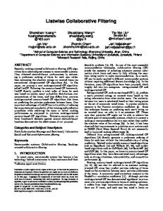
vector1 vector2 vector3

item1 item2 …… ⏀(M) Kernel function

Vu

MLP

Item vector

User vector SVD

Vi

score

R

Figure 1: Framework of our algorithm.

or items. With the vectors of user or items mapped to the network, some latent relationship between them can be discovered. For example, Shameem Ahamed Puthiya Parambath et al. put forward a method applied to recommendation systems based on the similarity graph [11]. Li Xin et al. proposed a method based on graph kernel to learn the relationship between the users and items [19]. Yuan Zhang et al. proposed a method based on graph and the label applying to recommendation systems [20]. The successful experiment results of these methods show the CF based on graph that has some advantages compared to the existing methods [1], because they can learn more latent information in the network [13]. However, most of the methods based on the graph are nonlinear, which predict the users’ ratings of unknown items by using a single classifier. We proposed an improved method based on graph for recommendation systems: first, we map the users’ information into vectors representation and transform the highdimensional vectors into low-dimensional vectors by the SVD decomposition [21], which can concentrate the vectors of the users’ information. We use the improved kernel function to compute the correlation between users [22]. Then the users’ vectors are mapped to the network and learn the relationship between users. We filter out other users who are similar to the given user. Next, the interests and preference of other similar users are analyzed, and the interaction between users and items is learned to make predictions through Multilayer Perceptron (MLP) method [23]. Finally, we predict the unknown rating and sort the items and recommend TopN to the user.

Compared with the existing CF methods [1], our method has some advantages and innovation, as follows: (1) Our method learns the correlation between users and items based on the graph [16], and more potential relationships can be discovered in the network [24]. Furthermore, compared with the existing methods based on graph, our method firstly uses the SVD method to reduce dimensions for the vectors of users’ information. It can not only reduce the amount of calculation to shorten the time but also enrich the vector of users. (2) We use the improved kernel method [22] which learns from Skip-gram model [25] to analyze more latent information by decomposition of the substructures. (3) Our method uses the MLP method to learn the latent features further. Our method is different from existing methods, which directly map the features of similar users to the classifier. We used the MLP learning method to learn the relationship between users and items to predict the rating of items [23]. The framework of our algorithm is shown in Figure 1.

2. Background and Related Work The recommendation systems benefit people in their daily lives. However, many of the recommendation algorithms face the problem of sparsity that performs poorly. Wei Zeng proposed a method based on the semilocal diffusion process


3

on the user-object bipartite network which improves the accuracy of the algorithm greatly [26]. In general, Static user-item networks may ignore the long-term impact. We often used heterogeneous models to learn users’ behavior patterns and improve performance by balancing optimization models and relational models [27]. Recommendation algorithms search for similar users through clustering methods or computing correlations. Ming-Sheng Shang proposed cooperative clustering coefficients to describe the selection mechanism of users and quantify the clustering behavior based on collaborative selection [28]. 2.1. Kernel Function. In many fields, such as social networks [29] and chemicals, we often need to calculate the similarities between the internal components and then find out some potential relationships between them. The graph represents the overall structure. We consider computing the correlation between nodes to explore some latent features. In the network, the node represents the users and the edge indicates whether there is a connection between them. There is a popular method for calculating the similarity between the object components by use of kernel methods [30]. In general, kernel methods use kernel functions to calculate the correlation between components [31]. The setting of proper kernel function is important for calculating the correlation because different structures adapt to different calculations [32]. In the graph, let the kernel function 𝐾(𝑉𝑖 , 𝑉𝑗 ) compute the correlation between nodes. Let 0(𝑉𝑖 ) represent the vector of node 𝑉𝑖 and let H represent dot product operation. This method of kernel function can capture the potential relationship between nodes. In the graph, the node is represented by the vector which contains the information of nodes. The kernel function between two nodes 𝑉𝑖 and 𝑉𝑗 can be given by 𝐾 (𝑉𝑗 , 𝑉𝑗 ) =< 0 (𝑉𝑖 ) , 0 (𝑉𝑗 ) > 𝐻

(1)

This is the common kernel function for the graph to calculate the relationship between nodes. However, we propose an improved kernel function learnt from the language model [33]. 2.2. Skip-Gram Model. Our approach learns from the Skipgram model to compute the probability [34]; then we introduce the background about the Skip-gram model [35]. The Skip-gram model represents the words by calculating the probability that a word and its surrounding words appear simultaneously in a sentence [36]. The objective of the method is not to predict the current word according to the surrounding words but to predict the surrounding words by the current word. Given the words {𝑤𝑖 }𝑘𝑖=1 from a sequence, the aim of the Skip-gram model is to maximize the following equation: 𝑇

∑ log Pr (𝑤𝑡−𝑐 , . . . , 𝑤𝑡+𝑐 | 𝑤𝑡 ) 𝑡=1

(2)

Pr(𝑤𝑡−𝑐 , . . . , 𝑤𝑡+𝑐 | 𝑤𝑡 ) is computed as follows: ∏ −𝑐≤𝑗≤𝑐,𝑗=0̸

Pr (𝑤𝑡+𝑗 | 𝑤𝑡 )

(3)

Here, it is assumed that the current and the surrounding words are dependent. Therefore, Pr(𝑤𝑡+𝑗 | 𝑤𝑡 ) is defined: exp (𝑉𝑤𝑇𝑡 𝑉𝑤󸀠 𝑡+𝑗 ) 𝑇 󸀠 ∑𝑉 𝑤=1 exp (𝑉𝑤𝑡 𝑉𝑤 )

(4)

where 𝑉𝑤 represents the input vectors of word 𝑤 and 𝑉𝑤󸀠 represents the output vectors. Hierarchical softmax is an efficient algorithm used to train the Skip-gram model [34]. It uses the binary Huffman tree for decomposition; the Huffman tree is the partition function of the Skip-gram model. Then it maps the similar words to similar positions in the vector spaces. The Skipgram model considers the substructure in the kernel function as a word in the sentence and uses the word embedding to represent the similarity between substructures.

3. Method We first define the basic notations that will be used in the paper. Then, we introduce the concept and function of the graph in our method and explain the process of the learning of the correlation based on the improved kernel function between users in the network. With the algorithm of Graph Kernel Method (GKM), we compute the feature vectors of users and items. Finally, we introduce the MLP, which learns the interaction between users and items to predict the rating. 3.1. Notations. Let 𝑈 represent a set of users; let I represent a set of items and let 𝑅 represent a set of the rating of users for items: R= {𝑅𝑖𝑗 ∈ 𝑅 | 𝑖 ∈ 𝑈, 𝑗 ∈ 𝐼}. Let G = (V, E) represent a graph, where 𝑉 is a set of vertices; 𝐸 ⊆ (𝑉 × 𝑉) is a set of edges in the graph; and 𝐺 is an undirected graph with nodes 𝑉 and edges E. |𝑉| represents the total number of the nodes. The adjacency matrix 𝐴 of the graph 𝐺 is defined as {0 𝐴={ 1 {

if (𝑢, V) ∈ 𝐸 𝑜𝑡ℎ𝑒𝑟𝑤𝑖𝑠𝑒

(5)

In the graph, 𝑉𝑖 {𝑖 | 𝑖 ∈ 𝑉} represents the user, and the edge 𝑒𝑖𝑗 {𝑖, 𝑗 | 𝑖 ∈ 𝑉, 𝑗 ∈ 𝑉} describes the interaction between 𝑉𝑖 and 𝑉𝐽 . In Table 1, we summarize the important notations throughout this paper. 3.2. Improved Kernel Function. Our approach uses the Skipgram model [32] to learn the latent features of substructures and represents the similarity between nodes by the corpus generation [33]. The method learns the features of nodes by a matrix [37] that represents the similarity between substructures, and the matrix is calculated by the vectors of the substructures. Then we learn the representation of the substructures through the Skip-gram model.

4

Mathematical Problems in Engineering (1) Input: Rating Matrix: R, 𝑅 ∈ 𝑅𝑚×𝑛 The dimension of feature: K (2) Procedure: (3) Decompose matrix 𝑅 with SVD method. 𝑅 󳨀→ 𝑃 ∈ 𝑅𝑚×𝑘 , 𝑄 ∈ 𝑅𝑛×𝑘 (4) For all user 𝑢 do (5) Receive the vector of V𝑢 (6) Compute the similarity between users with Equation (6) (7) end for (8) Through the activation function and compute the adjacency matrix A (9) Establish graph (10) For all user 𝑢 do (11) Traverse graph and receive the neighbors w (12) Compute the feature vector of 𝑝𝑢 with V𝑢 , w (13) end for (14) Output: The feature vector of user: 𝑝𝑢 The vector of item: 𝑞𝑖 Algorithm 1: GKM. Table 1: Notations.

𝑁V 𝑓V 0 (V) K(𝑉𝑖 , 𝑉𝐽 ) Pr(𝑤𝑡 ) 𝑉𝑤 𝑊𝑥 𝑏𝑥 𝑎𝑥

the set of neighbor nodes of node V the vector of node V the eigenvalue of node V in low dimension kernel function the possibility of 𝑤𝑡 the input vectors of word w the weight matrix the bias vector the activation function for every layer

Our framework lists a set of 𝑈 and decomposes them into substructures to compute the similarity between users. Then each substructure of decomposition is regarded as a sentence, and this sentence is generated by vocabulary 𝑉. In this vocabulary, vocabulary 𝑉 is corresponding to the training data observed in the unique set of substructures. However, different from the words in the traditional text corpus, there is no linear cooccurrence relationship between the substructures. Therefore, we need to establish a corpus, and it is meaningful to coexist in this corpus. Next, we will discuss how to generate a meaningful corpus of common occurrence relationships. In the graph, even a medium-size graph is pretty expensive for exhaustive enumeration. In order to adopt the sampling subgraphs effectively, several sampling heuristic algorithms are proposed such as biased random sampling and random sampling scheme. In practice, the random sampling of graphlets of size 𝑘 in a graph 𝐺 involves placing a randomly generated window of size 𝑘 × 𝑘 on the adjacency matrix of 𝐺 and collecting the observed graphlet in that window. This process is repeated 𝑛 times, where 𝑛 is the number of graphs we want to sample. However, because this is a random sampling percept, it does not retain any concept of cooccurrence, which is the desired attribute of our framework. Therefore, we make use of the concept of neighborhood and modify the random sampling percept, so that we can partially preserve the coexistence relationship between them. In other words, whenever we randomly select

a user, we also sample its neighbor. Users and their neighbors are interpreted as a common occurrence of our methods. Therefore, users with similar neighbors will receive similar representations. In this paper, we use the neighbor, which can extend the coexistence relationship to the neighborhood of distance ≥1. For verification, we discussed the influence of similar patterns in the language model and in the graph. We proposed the combination objective as follows: argmax 𝑎∗ ,𝑏∗ ∈𝑉

cos (𝑏∗ , 𝑏) cos (𝑏∗ , 𝑎∗ ) cos (𝑏∗ , 𝑎) + 𝛼

(6)

where 𝑎 and 𝑏 represent the substructures from the vocabulary V; 𝑎∗ and 𝑏∗ represent the related substructures which are similar to substructures a and b. And cos(⋅) is the function used to compute the similarity between the vectors of substructures. 𝛼 = 0.001 is a parameter to prevent that the division is zero. Then we normalize 𝐾(𝑉𝑖 , 𝑉𝑗 ) in the range (0, 1) and take it into an activation function. If the output from the activation function exceeded the threshold value(S), then A𝑖𝑗 =1; otherwise, A𝑖𝑗 =0. The size of the threshold value is determined by the parameter S; the setting of S is through supervised learning [35]. We proposed the Algorithm 1 of GKM to compute the feature vectors of users and items. 3.3. MLP. In general, a vector connection does not consider any interaction about the latent features between the users and items, and the effect is not sufficient for the model of CF. To solve this issue, as for the concatenated vectors, we propose to add hidden layers and use the standard MLP method [23] to learn the latent features between users and items. In this term, we can give the model a lot of flexibility and nonlinearity to learn the interaction between 𝑝𝑢 and q𝑖 , instead of using only fixed elements. The MLP model is defined as follows: 𝑧1 = 01 (𝑝𝑢 , 𝑞𝑖 ) = [

𝑝𝑢 𝑞𝑖

]

02 (𝑧1 ) = 𝑎2 (𝑊2𝑇𝑧1 + 𝑏2 )

(7) (8)


5

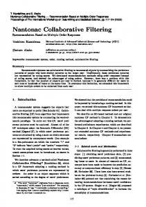
Input layer

Embedding layer

Latent Vector Vu

Vi

Layer 1

Layer 2

Neural layer

Layer y n

target

train score

Output layer

Figure 2: The framework of MLP.

... 0𝐿 (𝑧𝐿−1 ) = 𝑎𝐿 (𝑊𝐿𝑇𝑧𝐿−1 + 𝑏𝐿)

(9)

𝑦𝑢𝑖 = 𝜎 (ℎ𝑇0𝐿 (𝑧𝐿−1 ))

(10)

where 𝑊𝑥 represents the weight matrix; 𝑏𝑥 represents the bias vector; and 𝑎𝑥 represents the activation function of the perceptron for the xth layer. For 𝑎𝑥 , the activation functions of layers, the functions can be selected freely such as sigmoid, Rectified Liner Units (ReLU), and hyperbolic tangent (tanh). Here, we analyze these functions. (1) The sigmoid function limits each neuron in (0,1), which may limit the performance of the model. It is known that neurons stop learning when their output approaches 0 or 1. (2) tanh as a better choice has been widely adopted, but it only alleviates the problems of sigmoid in some degree, because it is as a cancelled version of sigmoid (tanh(x/2) = 2𝜎(x) − 1). (3) Finally, we choose ReLU, which is more reasonable and is proven to be unsaturated. In addition, ReLU encourages sparse activation, which is suitable for sparse data [38], and makes the model less likely to be overfitting. Our empirical results show that the performance of ReLU is better than the result of tanh, and tanh is better than sigmoid. To design the network structure, a common solution is to follow the pattern. The bottom of the layer is the widest and it has a small number of neurons for each successive layer. The premise is that they can learn more latent feature by using a

small amount of hidden units to higher units. We implement the tower structure in an empirical way, halving the size of layers per layer. The framework of MLP method is shown in Figure 2.

4. Experiments In this section, the extensive experiments are conducted in detail to evaluate the effectiveness of our algorithm on the different data sets. 4.1. Data Sets. To demonstrate the performance of our algorithm, the experiments are conducted on four public data sets, MovieLens100K(ML 100K), MovieLens1M(ML 1M), MovieLens10M(ML 10M), and MovieLens20M(ML 20M). The four data sets are collected from the MovieLens website (https://grouplens.org/datasets/movielens). 4.2. Evaluation Metrics. To evaluate the performance of our algorithm, we use two evaluation metrics: recall and F1. In detail, we regard the top 𝑃 as the recommended items for each user and sort them by the ratings. Then evaluation metrics are defined as follows: 𝑃 precision = 𝑁 recall = F1 =

𝑃 𝑇

2 × 𝑝𝑟𝑒𝑐𝑖𝑠𝑖𝑜𝑛 × 𝑟𝑒𝑐𝑎𝑙𝑙 𝑝𝑟𝑒𝑐𝑖𝑠𝑖𝑜𝑛 + 𝑟𝑒𝑐𝑎𝑙𝑙

(11)

6

Mathematical Problems in Engineering ML 100K

0.25

0.25

0.2

0.2

0.15

0.1

0.05

0.05 5

0

10 15 20 25 the number of recommended items

10 15 20 the number of recommended items

LDA

Graph+MLP

LDA

SVD

KNN+GBDT

SVD

CMF

UCF

CMF

UCF

KNN+Bayes

ICF

KNN+Bayes

ICF

ML 10M

0.3

0.25

0.2

0.2 F1

0.15

0.15

0.1

0.1

0.05

0.05 5


25

ML 20M

0.3

0.25

0

5

KNN+GBDT

Graph+MLP

F1

0.15

0.1

0

ML 1M

0.3

F1

F1

0.3

0

5

10 15 20 the number of recommended items

Graph+MLP

LDA

Graph+MLP

LDA

KNN+GBDT

SVD

KNN+GBDT

SVD

CMF

UCF

CMF

UCF

KNN+Bayes

ICF

KNN+Bayes

ICF

25

Figure 3: F1 of four data sets.

where P represents the number of items that the user likes in the top P; T represents total number of items which is related to the user; N represents the total number of items on the recommendation list. 4.3. Baseline Approaches. We list the models that are compared to our algorithm as follows: Graph+MLP: we use the structure of graph and MLP method to compute the similarity and predict the rating. LDA: the method treats the item as a word and regards the user as a document to compute the probability for recommendation [37]. CMF: Collective Matrix Factorization is a model to incorporate different sources of information by simultaneously factorizing multiple matrices [35]. KNN+GBDT: it uses KNN to find the similar users and gets the information about them. Then it uses the GBDT model to predict the ratings for items [5].

KNN+Bayes: similar to the model we described above, it searches the similar users and predicts the ratings by Bayes model [12]. SVD: SVD is a model of CF based on features. The useritem matrix is decomposed into two matrices, U and I, and then they are used to predict ratings directly [21]. UCF: users-based CF uses KNN to calculate the users’ correlation and recommends the items that similar users may like to the user. ICF: items-based CF uses KNN to calculate the items’ correlation and recommends the similar items to the user. 4.4. Results and Analysis. To empirically evaluate our algorithm, we compare our algorithm with all baselines we listed above on the real-world data sets. First, we split the data sets into train set and test set, with a ratio of 7:3. The effects of the experiment are as follows. Figure 3 shows F1 to measure the performance of all algorithms in four data sets. We can see that our proposed

0.5 0.45 0.4 0.35 0.3 0.25 0.2 0.15 0.1 0.05 0

7

recall

ML 100K

5


ML 1M

0.5 0.45 0.4 0.35 0.3 0.25 0.2 0.15 0.1 0.05 0

5

10

15

20

Graph+MLP

LDA

Graph+MLP

LDA

KNN+GBDT

SVD

KNN+GBDT

SVD

CMF

UCF

CMF

UCF

KNN+Bayes

ICF

KNN+Bayes

ICF

ML 10M

5

10

15

20

25

the number of recommended items

25

the number of recommended items

recall

0.5 0.45 0.4 0.35 0.3 0.25 0.2 0.15 0.1 0.05 0

recall

recall


0.5 0.45 0.4 0.35 0.3 0.25 0.2 0.15 0.1 0.05 0

ML 20M

5


Graph+MLP

LDA

Graph+MLP

LDA

KNN+GBDT

SVD

KNN+GBDT

SVD

CMF

UCF

CMF

UCF

KNN+Bayes

ICF

KNN+Bayes

ICF

Figure 4: The recall of four data sets.

Graph+MLP algorithm performs better in the ML 100K data set than other baseline methods in different number of recommend items. It is obvious that only use of KNN method for collaborative filtering is weaker than other algorithms whether based on users or items. Those algorithms that use KNN as preprocessing and classification to predict ratings can make a great effect. We can see that the effects of the KNN+GBDT and KNN+Bayes are better than UCF and ICF. For the KNN+GBDT and KNN+Bayes algorithms, with the same data preprocessing, the algorithm using Bayes classifier is better than the GBDT classifier, because the data set is too sparse with noise, which is not suitable for GBDT classifier. On the contrary, Bayes classifier is more suitable to predict ratings for the data set. Our algorithm used the graph method as preprocessing and then used the MLP method to predict ratings for the items. Our algorithm can perform better than the algorithms that use KNN as a preprocessing and input the prepared data to the classifier. We can see the performance effect in different data sets in Figure 3. In the data set of ML

100K, the effect of UCF is likely to ICF. However, there are larger data volumes in ML 1M, ML 10M and ML 20M. The effect of ICF in ML 20M is better than UCF, because the data set has small data volume; the ratio of the number of users to the number of items will be smaller. However, ICF algorithm is the opposite and it performs well when the ratio of the number of users is more than the number of items. On the ML 10M and ML 20M data sets, comparing our algorithm with the Bayes algorithm, when the value of p is 5, our algorithm does not perform better. With the value of p becoming larger, our algorithm performs better. On the four data sets, the performance of the CMF algorithm is the worst. Figure 4 shows the recall to measure the performance of all algorithms on four data sets. We can see that our algorithm performs best regardless of different data sets with the value of p. Combined with the results shown in Figure 3, we can conclude that our algorithm performs best in both accuracy and recall. According to the results of Figure 3, data is prepared with KNN algorithm and classifier is used

Mathematical Problems in Engineering ML 100K

0.4 0.35 0.3 0.25 0.2 0.15 0.1 0.05 0

0.35 0.3 0.25 0.2 0.15 0.1 0.05 50

60 70 training set ratio (%)

0

80

60

70

80

training set ratio (%)

LDA

Graph+MLP

LDA

KNN+GBDT

SVD

KNN+GBDT

SVD

CMF

UCF

CMF

UCF

KNN+Bayes

ICF

KNN+Bayes

ICF

ML 10M

ML 20M

0.4

0.3

0.35 0.3

0.25 0.2

recall

recall

50

Graph+MLP

0.35

0.15 0.1

0.25 0.2 0.15 0.1

0.05 0

ML 1M

0.4

recall

recall

8

0.05 50

60

70

80

0

50


60

70

LDA

Graph+MLP

LDA

KNN+GBDT

SVD

KNN+GBDT

SVD

CMF

UCF

CMF

UCF

KNN+Bayes

ICF

KNN+Bayes

ICF

Graph+MLP

80


Figure 5: The recall of different training set ratio.

to predict ratings. The effects of KNN + GBDT and KNN + Bayes are better than the KNN. Further, the effect of the KNN + Bayes is better than the KNN + GBDT in most of p values. Figure 5 shows the relationship between the recall and training ratio. We can see from that that our algorithm performs better than baseline algorithms in most cases. On the ML 100K dataset, our algorithm’s performance effect is worse than that of other datasets. The ML 100K dataset is too sparse, which has a large impact on the algorithm. In general, with the increase of data, the performance of all algorithms will improve. In the case of small training samples, our algorithm can perform better than other algorithms. What is more, as the amount of data increases, our algorithm’s performance will be improved faster than other algorithms. Our algorithm can adapt to large-scale data sets better than other algorithms. Table 2 shows the execution time of all algorithms in four data sets. We used ML 1M data set to test with 70%

data in train and 30% data in test. The main equipment in the experiment included E5 processor, GPU (GTX-1060), and 8 GB memory. We calculated the time including data preprocessing and model prediction. We can see from Table 2 that if our algorithm does not use SVD method to reduce the dimensions, it needs more time to complete the whole process. Especially with the increase of data sets, the gap between our algorithm and other algorithms is becoming more obvious. The complexity of our decomposition of subgraph in graph method will increase exponentially with the increase of the amount of data. But the speed of our algorithm with SVD is faster than the Graph+MLP without SVD regardless of our value of K in 10 or 15 on all of the data sets. Among all the classifier algorithms, our algorithm performs the fastest except for KNN + Bayes. We can see that the classifiers have a great effect on the accuracy of these algorithms. The performance of the UCF and ICF algorithm without the classifier is worse than KNN+GBDT


9

Table 2: The execution time of all algorithms in different data sets. Algorithm Graph+MLP (without SVD) Graph+MLP KNN+GBDT KNN+Bayes CMF LDA SVD UCF ICF

ML 100K

ML 1M

ML 10M

ML 20M

k=10

k=15

k=10

k=15

k=10

k=15

k=10

k=15

2.01

3.12

4.97

8.61

10.28

16.34

23.72

33.25

1.21 2.12 0.91 1.12 1.23 1.02 0.87 0.92

2.01 3.31 1.87 2.11 2.23 1.91 1.31 1.52

3.31 5.11 2.98 3.51 3.71 3.02 2.72 2.88

5.12 6.31 4.67 5.33 5.87 4.71 4.32 4.41

8.12 9.15 7.21 8.44 8.81 7.31 6.98 7.05

10.26 11.58 10.07 10.51 10.79 10.13 10.01 10.12

15.11 17.43 14.87 15.67 15.98 15.03 13.97 14.01

19.51 21.18 18.91 19.32 19.83 19.21 17.61 17.76

and KNN+Bayes. We used the SVD method to reduce the dimensions in data preparing, which can improve the speed of our algorithm.

5. Conclusions and Future Work In this paper, we proposed a CF model based on graph for recommendation systems. We improve the traditional graph model and use the kernel method to compute the relationship between users. Based on the improved kernel method, the similarity is calculated by the generation of the corpus of the Skip-gram model. By using the kernel method, the relation between users can be calculated and more latent information between users can be mined. On the other hand, the MLP method is adopted on the basis of the graph in our model. The method maps the vectors of users and items to neural network and learns more latent information between users and items by the operation of neurons. Therefore, compared with the baseline methods, our proposed model can achieve higher accuracy and recommendation effects. The items recommended by our model are more suitable for users. Well, in future work, we will further improve our model in several ways. First, we optimize the MLP method to mine more latent information between the users and items. Then, we optimize the time complexity and extend the method to online. Finally, with the rapid development of ecommerce, the time consumption of the recommendation is very important for users. So, we will consider applying it to the online recommendation systems.

Data Availability The data that support the findings of this study are openly available at https://grouplens.org/datasets/movielens.

Conflicts of Interest The authors declare that they have no conflicts of interest.

Acknowledgments The work was supported by the National Natural Science Foundation of China (no. 61502402) and the

Fundamental Research Funds for the Central Universities (no. 207220180073).

References [1] J. L. Herlocker, J. A. Konstan, L. G. Terveen, and J. T. Riedl, “Evaluating collaborative filtering recommender systems,” ACM Transactions on Information and System Security, vol. 22, no. 1, pp. 5–53, 2004. [2] S. H. Chee, J. Han, and K. Wang, “RecTree: an efficient collaborative filtering method,” in Data Warehousing and Knowledge Discovery, vol. 2114 of Lecture Notes in Computer Science, pp. 141–151, Springer Berlin Heidelberg, Berlin, Heidelberg, 2001. [3] Z. Zhang, Y. Kudo, and T. Murai, “Neighbor selection for userbased collaborative filtering using covering-based rough sets,” Annals of Operations Research, vol. 256, no. 2, pp. 359–374, 2017. [4] X. Zhou and S. Wu, “Rating LDA model for collaborative filtering,” Knowledge-Based Systems, vol. 110, pp. 135–143, 2016. [5] D. Adeniyi, Z. Wei, and Y. Yongquan, “Automated web usage data mining and recommendation system using K-Nearest Neighbor (KNN) classification method,” Applied Computing and Informatics, vol. 12, no. 1, pp. 90–108, 2016. [6] J. Liu, M. Tang, Z. Zheng, X. Liu, and S. Lyu, “Locationaware and personalized collaborative filtering for web service recommendation,” IEEE Transactions on Services Computing, vol. 9, no. 5, pp. 686–699, 2016. [7] X. Zhou, W. Shu, F. Lin, and B. Wang, “Confidence-weighted bias model for online collaborative filtering,” Applied Soft Computing, vol. 70, pp. 1042–1053, 2018. [8] A. P. Henriques, S. D. Castro, P. Joatilde, M.-M. Joatilde, and R. L. Paulo, “Using model-based collaborative filtering techniques to recommend the expected best strategy to defeat a simulated soccer opponent,” Intelligent Data Analysis, vol. no. 5, pp. 973– 991, 2014. [9] N. Quoc, P. Hoai, and H. Xuan, “Statistical implicative similarity measures for user-based collaborative filtering recommender system,” International Journal of Advanced Computer Science and Applications, vol. 7, no. 11, 2016. [10] A. Sattar, M. A. Ghazanfar, and M. Iqbal, “Building Accurate and Practical Recommender System Algorithms Using Machine Learning Classifier and Collaborative Filtering,” Arabian Journal for Science and Engineering, vol. 42, no. 8, pp. 3229– 3247, 2017. [11] S. A. P. Parambath, N. Usunier, and Y. Grandvalet, “A coveragebased approach to recommendation diversity on similarity

10

[12]

[13]

[14]

[15]

[16]

[17]

[18]

[19]

[20]

[21]

[22]

[23]

[24]

[25]

Mathematical Problems in Engineering graph,” in Proceedings of the 10th ACM Conference on Recommender Systems, RecSys 2016, pp. 15–22, USA, September 2016. L. M. de Campos, J. M. Fernández-Luna, J. F. Huete, and M. A. Rueda-Morales, “Combining content-based and collaborative recommendations: a hybrid approach based on Bayesian networks,” International Journal of Approximate Reasoning, vol. 51, no. 7, pp. 785–799, 2010. M. Rossetti, F. Stella, and M. Zanker, “Towards explaining latent factors with topic models in collaborative recommender systems,” in Proceedings of the 24th International Workshop on Database and Expert Systems Applications, DEXA 2013, pp. 162– 167, Czech Republic, August 2013. S. Zhang, L. Yao, and X. Xu, “AutoSVD++: An Efficient Hybrid Collaborative Filtering Model via Contractive Auto-encoders,” in Proceedings of the the 40th International ACM SIGIR Conference, pp. 957–960, Shinjuku, Tokyo, Japan, August 2017. X. Liu, C. Aggarwal, Y.-F. Li, X. Kong, X. Sun, and S. Sathe, “Kernelized matrix factorization for collaborative filtering,” in Proceedings of the 16th SIAM International Conference on Data Mining 2016, SDM 2016, pp. 378–386, USA, May 2016. J. Wasilewski and N. Hurley, “Intent-aware diversification using a constrained PLSA,” in Proceedings of the 10th ACM Conference on Recommender Systems, RecSys 2016, pp. 39–42, USA, September 2016. M. Agathokleous and N. Tsapatsoulis, “Voting advice applications: missing value estimation using matrix factorization and collaborative filtering,” in Artificial Intelligence Applications and Innovations, vol. 412 of IFIP Advances in Information and Communication Technology, pp. 20–29, Springer Berlin Heidelberg, Berlin, Heidelberg, 2013. M. Tang, Z. Zheng, G. Kang, J. Liu, Y. Yang, and T. Zhang, “Collaborative web service quality prediction via exploiting matrix factorization and network map,” IEEE Transactions on Network and Service Management, vol. 13, no. 1, pp. 126–137, 2016. X. Li and H. Chen, “Recommendation as link prediction in bipartite graphs: A graph kernel-based machine learning approach,” Decision Support Systems, vol. 54, no. 2, pp. 880–890, 2013. Y. Zhang, N. Zhang, and J. Tang, “A Collaborative Filtering Tag Recommendation System based on Graph,” Applied Computer Systems, pp. 297–306, 2009. A. G. Akritas and G. I. Malaschonok, “Applications of singularvalue decomposition (SVD),” Mathematics and Computers in Simulation, vol. 67, no. 1-2, pp. 15–31, 2004. P. Yanardag and S. V. N. Vishwanathan, “Deep graph kernels,” in Proceedings of the 21st ACM SIGKDD Conference on Knowledge Discovery and Data Mining, KDD 2015, pp. 1365–1374, Australia, August 2015. X. He, L. Liao, H. Zhang, L. Nie, X. Hu, and T. Chua, “Neural Collaborative Filtering,” in Proceedings of the the 26th International Conference, pp. 173–182, Perth, Australia, April 2017. X. Du, L. Huang, and Y. Du, “Improve the collaborative filtering recommender system performance by trust network construction,” Journal of Electronics, vol. 25, no. 3, pp. 418–423, 2016. A. Lazaridou, N. T. Pham, and M. Baroni, “Combining language and vision with a multimodal skip-gram model,” in Proceedings of the Conference of the North American Chapter of the Association for Computational Linguistics: Human Language Technologies, NAACL HLT 2015, pp. 153–163, USA, June 2015.

[26] W. Zeng, A. Zeng, M. Shang, Y. Zhang, and A. Sánchez, “Information filtering in sparse online systems: recommendation via semi-local diffusion,” PLoS ONE, vol. 8, no. 11, p. e79354, 2013. [27] X. Shi, X. Luo, M. Shang, and L. Gu, “Long-term performance of collaborative filtering based recommenders in temporally evolving systems,” Neurocomputing, vol. 267, pp. 635–643, 2017. [28] M. Shang, L. Lü, Y. Zhang, and T. Zhou, “Empirical analysis of web-based user-object bipartite networks,” EPL (Europhysics Letters), vol. 90, no. 4, p. 48006, 2010. [29] D. Holgado Ramos, “Analyzing Social Networks,” Redes. Revista hispana para el análisis de redes sociales, vol. 27, no. 2, p. 141, 2016. [30] J. Alama, T. Heskes, D. Kühlwein, E. Tsivtsivadze, and J. Urban, “Premise selection for mathematics by corpus analysis and kernel methods,” Journal of Automated Reasoning, vol. 52, no. 2, pp. 191–213, 2014. [31] R. K. Beatson, W. zu Castell, and S. J. Schrödl, “Kernel-based methods for vector-valued data with correlated components,” SIAM Journal on Scientific Computing, vol. 33, no. 4, pp. 1975– 1995, 2011. [32] “Editorial: Kernel Methods: Current Research and Future Directions,” Machine Learning, vol. 46, no. 1–3, pp. 5–9, 2002. [33] D. Ganguly, D. Roy, M. Mitra, and G. J. F. Jones, “A word embedding based generalized language model for information retrieval,” in Proceedings of the 38th International ACM SIGIR Conference on Research and Development in Information Retrieval, SIGIR 2015, pp. 795–798, Chile, August 2015. [34] H. Peng, J. Li, Y. Song, and Y. Liu, “Incrementally learning the hierarchical softmax function for neural language models,” in Proceedings of the 31st AAAI Conference on Artificial Intelligence, AAAI 2017, pp. 3267–3273, USA, February 2017. [35] A. Salle, M. Idiart, and A. Villavicencio, “Matrix factorization using window sampling and negative sampling for improved word representations,” in Proceedings of the 54th Annual Meeting of the Association for Computational Linguistics, ACL 2016, pp. 419–424, Germany, August 2016. [36] Y. Shen, W. Rong, N. Jiang, B. Peng, J. Tang, and Z. Xiong, “Word Embedding Based Correlation Model for Question/Answer Matching,” Computer Science, pp. 3511–3517, 2016. [37] H.-B. Jeon and S.-Y. Lee, “Language model adaptation based on topic probability of latent dirichlet allocation,” ETRI Journal, vol. 38, no. 3, pp. 487–493, 2016. [38] F. Lin, X. Zhou, and W. Zeng, “Sparse online learning for collaborative filtering,” International Journal of Computers Communications & Control, vol. 11, no. 2, p. 248, 2016.

Advances in

Operations Research Hindawi www.hindawi.com

Volume 2018

Advances in

Decision Sciences Hindawi www.hindawi.com

Volume 2018

Journal of

Applied Mathematics Hindawi www.hindawi.com

Volume 2018

The Scientific World Journal Hindawi Publishing Corporation http://www.hindawi.com www.hindawi.com

Volume 2018 2013

Journal of

Probability and Statistics Hindawi www.hindawi.com

Volume 2018

International Journal of Mathematics and Mathematical Sciences

Journal of

Optimization Hindawi www.hindawi.com

Hindawi www.hindawi.com

Volume 2018

Volume 2018

Submit your manuscripts at www.hindawi.com International Journal of

Engineering Mathematics Hindawi www.hindawi.com

International Journal of

Analysis

Journal of

Complex Analysis Hindawi www.hindawi.com

Volume 2018


Stochastic Analysis Hindawi www.hindawi.com


Volume 2018

Volume 2018

Advances in

Numerical Analysis Hindawi www.hindawi.com

Volume 2018

Journal of


Volume 2018

Journal of

Mathematics Hindawi www.hindawi.com


Function Spaces Volume 2018


Volume 2018


Differential Equations Hindawi www.hindawi.com

Volume 2018

Abstract and Applied Analysis Hindawi www.hindawi.com

Volume 2018

Discrete Dynamics in Nature and Society Hindawi www.hindawi.com

Volume 2018

Advances in

Mathematical Physics Volume 2018


Volume 2018