Collinear cluster tri-partition: Kinematics constraints and stability of collinearity P. Holmvall,1, 2, ∗ U. K¨oster,2 A. Heinz,1 and T. Nilsson1 1
Department of Physics, Chalmers University of Technology, SE-41296 Gothenburg, Sweden 2 Institut Laue Langevin, 71 avenue des Martyrs, F-38042 Grenoble Cedex 9, France (Dated: April 17, 2018)
arXiv:1612.06583v2 [nucl-th] 6 Jan 2017
Background: A new mode of nuclear fission has been proposed by the FOBOS collaboration, called Collinear Cluster Tri-partition (CCT), suggesting that three heavy fission fragments can be emitted perfectly collinearly in low-energy fission. This claim is based on indirect observations via missing-energy events using the 2v2E method. This proposed CCT seems to be an extraordinary new aspect of nuclear fission. It is surprising that CCT escaped observation for so long given the relatively high reported yield, of roughly 0.5% relative to binary fission. These claims call for an independent verification with a different experimental technique. Purpose: Verification experiments based on direct observation of CCT fragments with fission fragment spectrometers require guidance with respect to the allowed kinetic energy range, which we present in this paper. Furthermore, we discuss corresponding model calculations which, if CCT is found in such verification experiments, could indicate how the breakups proceed. Since CCT refers to collinear emission, we also study the intrinsic stability of collinearity. Methods: Three different decay models are used that together span the timescales of three-body fission. These models are used to calculate the possible kinetic energy ranges of CCT fragments by varying fragment mass splits, excitation energies, neutron multiplicities and scission-point configurations. Calculations are presented for the systems 235 U(nth , f) and 252 Cf(sf), and the fission fragments previously reported for CCT, namely isotopes of the elements Ni, Si, Ca and Sn. In addition, we use semi-classical trajectory calculations with a Monte-Carlo method to study the intrinsic stability of collinearity. Results: CCT has a high net Q-value, but in a sequential decay, the intermediate steps are energetically and geometrically unfavorable or even forbidden. Moreover, perfect collinearity is extremely unstable, and broken by the slightest perturbation. Conclusions: According to our results, the central fragment would be very difficult to detect due to its low kinetic energy, raising the question of why other 2v2E experiments could not detect a missingmass signature corresponding to CCT. Considering the high kinetic energies of the outer fragments reported in our study, direct-observation experiments should be able to observe CCT. Furthermore, we find that a realization of CCT would require an unphysical fine-tuning of the initial conditions. Finally, our stability calculations indicate that, due to the pronounced instability of the collinear configuration, a prolate scission configuration does not necessarily lead to collinear emission, nor does equatorial emission necessarily imply an oblate scission configuration. In conclusion, our results enable independent experimental verification and encourage further critical theoretical studies of CCT. Keywords: Fission; Ternary Fission; Collinear Cluster Tri-partition; Trajectory calculations
I.
INTRODUCTION
Nuclear fission has been the focus of intense experimental and theoretical studies ever since its discovery almost 80 years ago [1–3]. Usually, fission results in two fragments (binary fission) with similar (symmetric fission) or dissimilar (asymmetric fission) masses. The possibility of fission into three fragments (ternary fission, see G¨ onnenwein et al. [4] for a review), was proposed [5] shortly after the discovery of binary fission. Experimental evidence of ternary fission was found 70 years ago in nuclear emulsion photographs [6, 7] and in measurements with ionization chambers [8]. Detailed investigations showed that ternary fission occurs once every
∗
[email protected]
few hundred fission events. In 90% of all ternary fission events, the third particle, called the ternary particle, is a 4 He nuclei, and in 9% hydrogen or a heavier helium nuclei. In only 1% of all ternary fission events does the ternary particle have Z > 2, with yields rapidly dropping with increased Z [9]. Ternary particles up to Z = 16 have been observed at yields of the order of 10−9 per fission [10]. However, early claims [11–15] for yet heavier ternary particles or even “true ternary fission” with three fragments of comparable masses remain disputed. Dedicated counting experiments searching for such events in planar geometry [16] and radiochemical experiments [17– 19] gave upper yield limits below 10−8 for true ternary fission. Therefore, it came as a great surprise when the FOBOS collaboration reported new experiments indicating true ternary fission events with a yield of 5 · 10−3 per fission [20–22]. These experiments were performed with
2 the fission fragment spectrometers FOBOS and miniFOBOS [23], in which detector modules are placed at opposite sides (180◦ angle) of a thin fission target. The fission target backing creates an intrinsic asymmetry of the setup since fragments detected in one of the arms have to traverse the backing. Binary coincidences from 252 Cf(sf) and 235 U(nth , f) were measured with this setup. The binary spectrum showed an enhancement of events with lower energy from the detector arm on the side of the target backing. Some of these missing energy events were interpreted as missing mass, that could correspond to a third particle missing detection due to scattering in the fission target backing. The claim was that three heavy fragments were emitted perfectly collinearly along the fission axis, the two lightest fragments in the same direction as the target backing, and the heavy in the opposite, and that the smallest of the three fragments (the ternary particle) did not reach the active area of the detector. Hence, this interpretation was dubbed “Collinear Cluster Tri-partition” (CCT). In the following, we will use this definition of CCT as collinear fission events with a relative angle between fragment emission directions of 180 ± 2◦ [20]. A similar experiment, but without an explicit asymmetry in any of the flight paths, was performed by Kravtsov and Solyakin [24], showing no indication of neither CCT nor missing mass events, down to a level of 7.5 · 10−6 per fission in 252 Cf(sf). Given these surprising results and the high reported yield of 0.5%, the fact that no indication of CCT was found before in neither radiochemical analysis, nor coincidence measurements, calls for an independent verification, preferably with a direct observation method. This is indeed possible, and under way, with the LOHENGRIN fission fragment recoil separator (to be reported in a future paper). For a verification experiment based on direct observation, it is crucial to know which kinetic energies to scan. Since the FOBOS collaboration did not report at which kinetic energies the fragments were measured, these kinetic energies need to be inferred from theory, which is the main focus of this paper. The kinetic energy distribution of one fragment in a ternary decay cannot be derived from first principles. Instead, the full range of kinetic energies allowed by energy and momentum conservation can be calculated, which is done in this study. This is straightforward since CCT is a one-dimensional decay in which the acceleration is repulsion dominated, yielding a limited amount of possibilities of how the kinetic energy can be distributed between the fragments. The possible kinetic energies are reduced even further by the constraint posed by the FOBOS experiments, that two of the fragments have a kinetic energy which is high enough to enter the detector arms and leave a clear signal. An experiment that can cover all the energies allowed by energy and momentum conservation can thus verify CCT model-independently. If events are found, our model calculations would indicate how the breakups proceed in CCT, by comparison with the measured kinetic energies.
We start this paper by detailing which fissioning systems will be studied. This is followed by a description of the theoretical models spanning the possible kinetic energies in CCT, and the Monte-Carlo method used to study the intrinsic stability of collinearity. Results are then presented in the form of possible final kinetic energies in CCT, benchmarks of the methods used, studies that highlight overlooked contradictions in the models currently favored in the literature, and studies of the stability of CCT. This is followed by discussions on verification of CCT by direct observation, on the CCT interpretation and on the intrinsic stability of CCT. Finally, the paper ends with conclusions and appendices with details of each model and method.
II.
FISSIONING SYSTEMS
In this paper, we present new and detailed calculations on the reported CCT clusters [20–22] 235
U(nth , f) → Sn + Si + Ni + ν·n, Cf(sf) → Sn + Ca + Ni + ν·n,
252
(1) (2)
both with and without intermediate steps leading up to the final fragments, where ν is the neutron multiplicity. Other speculated fragments have similar masses and Qvalues, and therefore similar kinematics. The derivations presented in this paper allow easy extension to any desired system. In the analysis of the FOBOS experiments [20–22], the measurements were interpreted as masses ASn ≈ 132 and ANi ≈ 68–72 with ν ≈ 0–4, with missing masses ASi ≈ 34–36 and ACa ≈ 48–52, respectively. These are the most energetically favorable masses, as shown in Fig. 1. Our study includes a slightly wider range of masses. The figure shows Q-values which are relatively high compared to binary fission. As our results will show, however, a high Q-value does not necessarily imply a high yield or probability for fission, since the intermediate steps may be unfavorable or forbidden.
III.
THEORETICAL MODELS
CCT is a decay in one spatial dimension, in which three fragments are formed from one fissioning system (FS) through two breakups [26, 27] and accelerated along the same line (see Fig. 2). If the time between breakups is long enough, there exists an intermediate state with a heavy fragment (HF) and an intermediate fragment (IF), the latter which splits in turn into a light fragment (LF) and a ternary particle (TP). The ternary particle here refers to the lightest fragment. If the time between breakups is sufficiently short, there is no intermediate state, and the decay is a “true” three-body decay. Therefore, for a given fissioning system, the essential parameter to describe CCT is the time between the two
3 breakups. In this paper, we divide the timescale of this parameter into three regimes, or models, and explicitly show that the kinetic energies of these models overlap in the limits. The first model is called the “sequential” decay model [28] and is based on two sequential binary fissions, with long timescales between the two successive scissions (i.e. assuming fully accelerated fragments before the second scission). The second model is the recently proposed “almost sequential” decay model [29], with intermediate timescales between scissions (assuming partially accelerated fragments before the second scission). These sequential models are the currently favored models in the literature. As is shown in the results, however, both of these models assume the fission of an intermediate system with a high fission barrier and extremely low (or even negative) Q-value. This motivates the study of a third model which is based on traditional ternary fission models, and called in the following the “true ternary” decay model, with “infinitesimal” timescales between scissions (i.e. no intermediate step or fragment). We mainly focus on the sequential and true ternary decay models, as they represent the extremes of the kinetic energy range, but we also show how to calculate all the possible kinetic energies allowed by energy and momentum conservation for all three models, for other fissioning systems as well. The final kinetic energies of the fission fragments are obtained analytically in the sequential decay model. This is possible since the kinematics in this model is fully determined by energy and momentum conservation. In the almost sequential and true ternary decay models, the final kinetic energies depend on the dynamics. Thus, these results are obtained with semi-classical trajectory calculations (see Wagemans [30] chapter 12-III for a review).
76 74 72 70 68 66 64
180
235 U(n
190
Q-value (MeV)
200
210
th,f) → Sn + Si + Ni
220
230
240
250
252 Cf(sf) → Sn + Ca + Ni
76 74 72 70 68 66 64
FS
1.
ANi
ANi
170
In these calculations, the scission configuration (initial fragment positions and momenta) is constrained by energy and momentum conservation for a given fissioning system. Subsequently, the final kinetic energies are calculated by starting from the scission configuration and solving the equations of motion iteratively. The latter is done with a fourth-order Runge-Kutta method using a time step of 10−25 s, until more than 99% of the potential energy is converted into kinetic energy. Since the 1960s, semi-classical trajectory calculations have been applied to ternary fission, mainly with the aim to determine the scission configuration [31]. As in many of these studies, a “point charge approximation” is used in our trajectory calculations, which assumes only a repulsive Coulomb force between spherical fragments. For the purpose of finding which scission configuration matches a particular final distribution, this method has received critique due to ambiguity [32–35], since several initial configurations can have the same final distribution. We do not have the same aim, however. Instead, we vary all possible initial collinear configurations in order to find all possible final kinetic energies of CCT fragments. Furthermore, we again stress the fact that in contrast to the previously mentioned studies, we study CCT which is a one-dimensional problem in which the dynamics during the fission fragment acceleration is dominated by the repulsive Coulomb interaction. Adding an attractive nuclear correction to the sequential model does not affect the final momenta, since the latter is uniquely determined by energy and momentum conservation. This is verified by the perfect agreement between our results and that of Vijayaraghavan et al. [28], who included an attractive nuclear correction. Still, we show explicitly that the attractive nuclear correction has a negligible effect in both the sequential and the almost sequential decay models (see Sec. IV B). In the true ternary decay model, the attractive nuclear interaction reduces the possible kinetic energy range (as discussed in Sec. III C). Since we are looking for the widest possible kinetic energy range to
(a)
(b)
28 30 32 34 36 38 40
ASi
44 46 48 50 52 54 56
ACa
FIG. 1. (Color online) Plots (a) and (b) show the Q-value versus the final mass split between the lightest fragments, in the decays in Eqs. (1) and (2), respectively, at zero neutron multiplicity (ν = 0). The Q-values are calculated from mass excesses taken from AME2012 [25]. No data are available for the bottom left corner (i.e. for masses ASn > 138). Prompt neutron emission ν > 0 generally lowers the Q-values (see Fig. 3).
2.
3.
IF
HF
HF
TP/LF
LF/TP
FIG. 2. (Color online) Schematic picture of the formation of CCT. For long timescales between two successive (sequential) breakups, there is an intermediate state (2). For sufficiently short timescales between breakups, there is no intermediate state, and the decay is a true three-body decay. Arrows indicate momentum direction. See text for explanation of acronyms.
4
Sequential decay model
In the sequential decay model [28], the fissioning system splits into a heavy fragment and an intermediate fragment. The latter splits in turn into a light fragment and a ternary particle. The ternary particle here refers to the lightest fragment. Either the TP or the LF can be formed at the center, as illustrated in Fig. 2. Potential energy surface calculations [29, 40, 41] predict that it is more likely that the TP is formed at the center. Nevertheless, we present results for both cases. Using conservation of proton numbers in Eqs. (1) and (2), the intermediate fragments are found to be molybdenum (Mo) and cadmium (Cd) in 235 U(nth , f) and 252 Cf(sf), respectively. Allowing for neutron emission from the FS and the IF with multiplicities ν1 and ν2 , respectively, gives 235
U(nth , f) → Sn + Mo + ν1 · n → Sn + Si + Ni + (ν1 + ν2 ) · n 252 Cf(sf) → Sn + Cd + ν1 · n → Sn + Ca + Ni + (ν1 + ν2 ) · n.
(3) (4)
The most energetically favorable masses of the IFs are found to be AMo = 104 and ACd = 120 with neutron multiplicity ν1 = 0, as seen in Figs. 3 (a) and (b), respectively. The most favorable mass split in the decay of 104 Mo is ANi = 70 and ASi = 34 with ν2 = 0, and in the decay of 120 Cd it is ANi = 70 and ACa = 50 with
Q-value (MeV)
A.
ν2 = 0, as seen in Figs. 3 (c) and (d), respectively. We will present final kinetic energies for a range of masses centered around these mass splits, with neutron multiplicities ν1 = 0–4. Note, however, that in the decay of both Mo and Cd, the Q-value is extremely low, for many mass splits even negative, and that any neutron multiplicity ν2 > 0 lowers the Q-value further. To have any chance of decaying, the IF needs excitation energy (from ∗ here on denoted EIF ). Even if the low Q-values are compensated for by an extremely high excitation energy, it does not mean that the intermediate fragment can fission, it also has to overcome a very high fission barrier (see Sec. V B for discussion). Therefore, we assume cold compact fission of the IF, by setting both the neutron multiplicity ν2 and the sum of the excitation energies of ∗ ∗ the final fragments TXE = EHF + ET∗ P + ELF to zero in our calculations. We show how to calculate a more general case, however, and such results can be directly obtained from our results by simple subtraction. Any TXE > 0 lowers the sum of the final kinetic energies accordingly, and any ν2 > 0 lowers the IF Q-value and the final total kinetic energy of the TP and LF by up to 8 MeV per neutron (see discussion in Sec. V B). The final kinetic energies of the fragments will be cal-
Q-value (MeV)
cover experimentally, the attractive nuclear interaction is excluded in this model to get a safe upper limit. In addition to deriving the possible final kinetic energies, we use a Monte-Carlo method to sample perturbations in the trajectory calculations, testing the intrinsic stability of collinearity in ternary fission, yielding the final angular distributions versus the perturbations. Previous studies using the point charge approximation with a Monte-Carlo approach successfully reproduced experimental ternary fission data [36, 37]. Furthermore, for the purpose of calculating final kinetic energies and angular distributions, it has been shown that the simple point charge approximation gives similar results to more sophisticated models, which incorporate attractive nuclear forces, fragment deformations and other effects [38, 39]. Nevertheless, to test the validity of our semi-classical trajectory calculations, we set up several benchmarks. As a quantitative verification against analytical calculations, the sequential and almost sequential models are compared for extremely long times between the two scissions, and the two techniques show excellent agreement (see results in Sec. IV A). Additional tests for ternary fission with 4 He (not reported here) reproduced well the results of the previously mentioned studies. We also verified for certain configurations that the inclusion of higher order moments corresponding to deformed fragments does not considerably affect the final momenta along the fission axis.
ASn + ν1
ASn + ν1
AMo
ACd
138 136 134 132 130 128 126 138 136 134 132 130 128 126 250 235 250 (a) U(nth,f) → Sn + Mo + ν1 ·n (b) 252 Cf(sf) → Sn + Cd + ν1 ·n 240 240 230 230 220 220 210 210 200 200 190 190 ν1 =0 ν1 =1 180 180 ν1 =2 ν1 =3 170 170 ν1 =4 160 160 98 100 102 104 106 108 110 114 116 118 120 122 124 126
30 20 10 0 10 20 30 40 50 60
ANi + ν2
76 74 72 70 68 66 64 (c) 104 Mo → Si + Ni + ν2 ·n
28 30 32 34 36 38 40
ASi
ANi + ν2
76 74 72 70 68 66 64 30 (d) 120 Cd → Ca + Ni + ν2 ·n 20 10 0 10 20 30 ν2 =0 ν2 =1 40 ν2 =2 ν2 =3 50 ν2 =4 60 44 46 48 50 52 54 56
ACa
FIG. 3. (Color online) The Q-value versus the mass split in the binary decays of (a) 235 U(nth , f), (b) 252 Cf(sf), (c) 104 Mo and (d) 120 Cd. The Q-values are calculated from the mass excesses, taken from AME2012 [25]. Lines have been added to guide the eye.
5 culated and presented versus fragment mass splits, neu∗ tron multiplicity and the excitation energy EIF . Details of this model are found in App. A.
B.
“Almost sequential” decay model
To calculate the kinematics of an “almost sequential” decay [29], a similar parametrization as in the sequential model is used. The main difference with respect to the sequential model is the finite time between the first and the second scission, which is analogous to the chargecenter distance between the HF and the IF at the second scission, denoted D (see Fig. 4). The finite time and distance makes it necessary to account for the Coulomb repulsion at all stages in the almost sequential model, thus the final kinetic energies depend on the full dynamics. To this end the scission-point configuration after the second scission is constrained, and the final kinetic energies are calculated from this configuration using semi-classical trajectory calculations (described in the beginning of this section). As will be shown in the results (Sec. IV B), an attractive nuclear interaction is found to have negligible influence on the final kinetic energies. Apart from the parameters of the sequential model (neutron multiplicities, fragment mass splits and excitation energies), the almost sequential model relies on two additional parameters to constrain the scission-point configuration. We choose these parameters to be the tip distances (surface separation distances) between the HF and the IF (∆D) at the moment of the second scission, and between the LF and the TP (∆d) after the second scission. The tip distance is defined as ∆Dij = Dij − Ri − Rj , (5) √ where Rk = r0 3 Ak is the radius of fragment k with mass Ak and r0 ≈ 1.25 fm, and Dij is the charge-center distance between the respective fragments. Note that as D, ∆D → ∞, the equations of the almost sequential decay model become exactly the same as those for the
FS
1.
2.
HF
ΔD
sequential decay model. Details of this model are found in App. A. As will be shown in the results (Sec. IV B), not even the most favorable mass splits will have enough energy to allow for a physically reasonable tip distance (< 4 fm [42]). Therefore, cold compact fission of the IF is assumed in our calculations, i.e. minimizing ∆d, by setting both the neutron multiplicity ν2 and the sum of the final ∗ ∗ fragment excitation energies TXE = EHF + ET∗ P + ELF to zero. As described in Sec. III A, results for ν2 > 0 and TXE > 0 can be obtained directly from our results.
C.
True ternary decay model
In the most common theoretical models of ternary fission (see Wagemans [30] chapter 12 and references therein), all three fragments are considered to be formed during a very short time interval from the same fissioning system, with the ternary particle at the center. The different models have a similar parametrization, but are based on different hypotheses and favor different starting positions of the ternary particle between the heavier fragments. Our true ternary decay model is based on the most common models, but is collinear, as is illustrated in Fig. 5. Furthermore, our model treats the ternary particle offset between the other fragments as a parameter, denoted xr . We let xr = 0 and xr = 1 correspond to the cases when the ternary particle is formed “touching” the heavy and light fragment, respectively. The results show that the highest kinetic energy for the LF is achieved if the TP is formed touching the HF. This is because the HF accelerates the TP, which then transfers momentum to the LF. The opposite configuration gives the lowest kinetic energy for the LF, and the highest possible for the HF. Obviously, these touching configurations are not real “scission” configurations, since in reality the fragments would not separate due to the attractive nuclear force. Therefore, the exploration from one touching configuration to the other will predict a wider kinetic energy range than physically possible. The touching configurations thus provide safe upper limits for the experimental search, which is why the attractive nuclear interaction is disregarded in this model. The scission-point configuration is constrained by energy conservation for given fragment mass splits, neutron multiplicity and pre-scission kinetic energies, with the pa-
IF
D
3.
HF
TP/LF
d Δd
LF/TP
FIG. 4. (Color online) CCT as an “almost sequential” decay. In contrast to the sequential model, the Coulomb repulsion of the heavy fragment is crucial after the second scission, making the inter-fragment distances relevant to the kinematics. Arrows indicate momentum direction.
FS
1.
2.
HF
xr
TP
LF
FIG. 5. (Color online) CCT as a true ternary decay. Arrows indicate momentum direction.
6 rameters xr and TXE , where the latter is the sum of the ∗ ∗ fragment excitation energies (TXE = EHF +ET∗ P +ELF ). Note that axial pre-scission kinetic energy can be canceled in most cases by choosing an earlier reference time, corresponding to a tighter scission configuration. We have therefore set the pre-scission kinetic energy to zero in our calculations. Lateral pre-scission kinetic energy is studied in Sec. III D, and is found to break collinearity, even for extremely low values. Using the scission-point configuration, the final kinetic energies are computed with semi-classical trajectory calculations, as described in Sec. III. Details of this model are found in App. B.
D.
Intrinsic stability of collinearity
Using the true ternary decay model (Sec. III C), the intrinsic stability of collinearity in ternary fission is analyzed by using a Monte-Carlo method to sample a perturbation in the ternary particle position and momentum perpendicular to the fission axis, independently (see Fig. 6). As in the true ternary decay model, the parameters are xr (the relative ternary particle position at scission, as described in Sec. III C) and TXE (the sum of the fragment excitation energies). In addition, a parameter representing the perturbation is also varied, being either initial lateral momentum or spatial offset of the ternary particle from the fission axis, denoted py and y, respectively. Given these parameters, the scission-point configuration is uniquely constrained by invoking conservation of energy, as well as linear and angular momentum. Each parameter is sampled in a uniform interval, with ∼ 100 sampling points per parameter, giving more than 106 data points per system. Using the scission-point configuration, the final kinetic energies and emission angles are computed with semiclassical trajectory calculations, as described in Sec. III. Details of this model are found in App. C.
FS
1.
2.
HF
xr y
LF TP py
FIG. 6. (Color online) CCT as a true ternary decay, with an initial lateral momentum or spatial offset of the ternary particle from the fission axis. The arrow indicates momentum direction.
IV.
RESULTS
The results are divided into four subsections. The first subsection covers final kinetic energies in the sequential decay model, both if the ternary particle is formed at the center (which is considered the most favorable case according to potential energy surface calculations [29, 40, 41]), and if the light fragment is formed at the center, for sake of completeness. The first subsection also includes a benchmark of the semi-classical trajectory calculations, which is used in the other models. The second subsection covers results for the “almost sequential” decay model, which show that this model spans the kinetic energy continuum between the sequential and “true ternary” decay models. Furthermore, it is explicitly shown that although CCT might have a high net Q-value, the intermediate steps in a sequential and an almost sequential decay are energetically and geometrically unfavorable or even forbidden. It is also shown that the attractive nuclear interaction is negligible in both the sequential models. The third subsection covers final kinetic energies in the true ternary decay model. The fourth subsection covers an analysis of the intrinsic stability of collinearity in ternary fission, in which the final scattering angle between the ternary particle and light fragment is presented versus a spatial and a momentum-based perturbation, independently. Requiring a collinear emission sets a threshold on the position and momentum of the ternary particle, which is shown to be much smaller than variations expected due to the uncertainty principle.
A.
Sequential decay results
Using the sequential model described in Sec. III A (derivations in App. A), we present in Figs. 7 (a)–(b) and (d)–(e) the final fragment kinetic energies versus the mass split between the TP and the LF in the decays 235
U(nth , f) → 132 Sn + 104 Mo → 132 Sn + Si + Ni (6) Cf(sf) → 132 Sn + 120 Cd → 132 Sn + Ca + Ni, (7)
252
respectively (note that the mass split between the HF and the IF will be varied later). For sake of completeness, results are presented for fission both when the (a),(d) TP and when (b),(e) the LF are formed at the center. Figs. 7 (c) and (f) show the Q-value in the fission of the intermediate fragments 104 Mo and 120 Cd, respectively. In both systems, the excitation energy of the interme∗ diate fragment is EIF = 30 MeV. As a benchmark of the semi-classical trajectory calculations, the figures also show results (+, ×) obtained from the almost sequential model (described in Sec. III B, derivations in App. A) at extremely long times between the two scissions. There is an excellent agreement between the two methods, as shown by the complete overlap of the symbols. The small
7
Q-value (MeV) -5
(a) Mo → Si + Ni
ASi
5
10
15
20
25
(b) Cd → Ca + Ni
20
28 30 32 34 36 38 40
0
44 46 48 50 52 54 56
76 74 72 70 68 66 64
ANi
-10
=1
ANi
-15
A Cd
76 74 72 70 68 66 64
-20
04 =1
difference is attributed to the fact that the trajectory calculations have to start and end with a finite potential energy (< 1%). The kinetic energy of the HF is labeled in each plot. The shape of the kinetic energy plot directly follows the Q-value in the fission of the intermediate fragment. For comparison, the Q-value in the fission of both Mo and Cd is shown as a function of the mass split between the TP and LF in Fig. 8. To have any probability of fissioning, only the most energetically favorable systems should be considered. Further calculations therefore assume that no neutrons originate from the fission of the IF (i.e. ν2 = 0 in Eqs. (3) and (4)), and that ∗ ∗ TXE = EHF +ET∗ P +ELF = 0 MeV. Any TXE > 0 MeV lowers the final kinetic energy sum accordingly. If any
-25
A Mo
FIG. 7. (Color online) Final kinetic energies of the TP and LF versus the TP to LF mass split in the sequential decay of (a)–(b) 235 U(nth , f) and (d)–(e) 252 Cf(sf), calculated with the analytic method ( , 4) described in Sec. III A (derivations in App. A), and with trajectory calculations (+, ×) described in Sec. III B (derivations in App. A). The case when the TP is formed at the center is shown in (a) and (d), while the case when the LF is formed at the center is shown in (b) and (e), (upper and lower signs in Eqs. (A30) and (A31), respectively). The corresponding final kinetic energy of the HF is labeled in each plot. The excitation energy of the intermediate fragment ∗ = 30 MeV. The missing trajectory calculations for is EIF ASi = 28 highlights that the intermediate steps of the decay are energetically forbidden. The corresponding Q-values in the fission of (c) 104 Mo and (f) 120 Cd are calculated from mass excesses taken from AME2012 [25]. Lines have been added to guide the eye.
neutrons are emitted in the fission of the IF, the Qvalue, and therefore the summed kinetic energy of the TP and LF, are reduced by up to 8 MeV per neutron. See Sec. V B for further discussion. To see how the kinetic energies are affected when vary∗ ing EIF and the mass split between the HF and the IF, multiple plots are compared to each other in a grid in Fig. 9, for both (a) 235 U(nth , f), and (b) 252 Cf(sf). Comparing plots in the horizontal direction, the heavy fragment mass is varied ASn = 134–130, and comparing ∗ plots in the vertical direction, EIF is varied (0, 20 and 40 MeV). The corresponding final kinetic energy of Sn and the varied parameters are labeled in each plot. Note that the results for 252 Cf(sf) in Fig. 9 (b) shows perfect agreement with the corresponding parameter choices in Fig. 6 of Vijayaraghavan et al. [28]. Increasing the exci∗ tation energy EIF frees more energy for the acceleration of the TP and LF. Because the direction of acceleration of the inner fragment is opposite to the flight direction of the IF before it fissions, the inner fragment is retarded. For higher excitation energies, the kinetic energy of the ∗ leaves inner fragment approaches 0 MeV. Increasing EIF less energy available as kinetic energy to the HF. Note that some of the corresponding systems are energetically forbidden for lower excitation energies and for unusual N/Z ratios. Results obtained with trajectory calculations (+, ×) only show fission decays which are energetically allowed and have a tip distance that is ≤ 7 fm at the second scission. None of the systems have a tip distance which is considered to be physically valid, i.e. less than 4 fm [42] (see Sec. IV B for results and discussion).
ACa
FIG. 8. (Color online) The Q-value as a function of the mass split between the LF and the TP, in the decays (a) Mo → Si + Ni and (b) Cd → Ca + Ni. Recall from Fig. 1 that masses under the dashed line correspond to nuclides without data for the corresponding HF (ASn > 138), and from Fig. 3 that the most favorable mass splits are ASn = 132 with (a) AMo = 104 and (b) ACd = 120. The most favorable mass split between the TP and LF are therefore found along the solid diagonal lines as ANi = 70 with (a) ASi = 34 and (b) ACa = 50. The Q-values are calculated from mass excesses taken from AME2012 [25]. Prompt neutron emission from the IF (ν2 ) lowers the Q-values significantly (see Fig. 3).
8
72 120
Ekin (MeV)
60
67
62
Energetically forbidden ASn=134 ∗ EMo =0 MeV
(a) 235 U(nth,f) → Sn + Mo → Sn + Si + Ni ANi
73
68
63
74
Energetically forbidden ASn=133 ∗ EMo =0 MeV
69
64
Energetically forbidden ASn=132 ∗ EMo =0 MeV
75
Ni Si 70
65
Energetically forbidden ASn=131 ∗ EMo =0 MeV
76
Ni Si 71
66
Energetically forbidden ASn=130 ∗ EMo =0 MeV
0 120 ASn=133 ESn=78.9 MeV ∗ EMo=20 MeV
ASn=132 ESn=81.9 MeV ∗ EMo=20 MeV
ASn=131 ESn=81.7 MeV ∗ EMo=20 MeV
ASn=130 ESn=83.2 MeV ∗ EMo=20 MeV
60
0 120
0 120
ASn=134 60 ESn=68.7 MeV ∗ EMo =40 MeV 30
73 150
35
68
ASn=133 ESn=70.2 MeV ∗ EMo =40 MeV 40
63
ASn=134
100
Ekin (MeV)
ESn=107.3 MeV 50 ECd∗ =0 MeV
30
74
35
ASn=132 ESn=73.1 MeV ∗ EMo =40 MeV 40
30
ASi
35
ASn=131 ESn=72.8 MeV ∗ EMo =40 MeV 40
30
(b) 252 Cf(sf) → Sn + Cd → Sn + Ca + Ni ANi 69
64
75
70
65
76
35
ASn=130 ESn=74.2 MeV ∗ EMo =40 MeV 40
30
35
40
Ni Ca 71
66
77
60
50
72
67 150
ASn=133
ASn=132
ASn=131
ASn=130
ESn=109.0 MeV ∗ ECd =0 MeV
ESn=112.6 MeV ∗ ECd =0 MeV
ESn=112.5 MeV ∗ ECd =0 MeV
ESn=114.6 MeV ∗ ECd =0 MeV
50 0
100 50 0 150
ASn=134 ESn=97.9 MeV ∗ ECd=20 MeV
ASn=133 ESn=99.6 MeV ∗ ECd=20 MeV
ASn=132 ESn=103.1 MeV ∗ ECd=20 MeV
ASn=131 ESn=102.9 MeV ∗ ECd=20 MeV
ASn=130 ESn=104.9 MeV ∗ ECd=20 MeV
0 150 100
0
Ni Ca
0 150 100
60 0 120
ASn=134 60 ESn=77.4 MeV ∗ EMo=20 MeV
0
120
100 50 0 150
ASn=134 ESn=88.6 MeV ∗ ECd =40 MeV 45
50
55
ASn=133 ESn=90.1 MeV ∗ ECd =40 MeV 45
50
55
ASn=132 ESn=93.6 MeV ∗ ECd =40 MeV 45
ACa
50
55
ASn=131 ESn=93.3 MeV ∗ ECd =40 MeV 45
50
55
ASn=130 ESn=95.3 MeV ∗ ECd =40 MeV 45
50
55
100 50 0
FIG. 9. (Color online) Final kinetic energies of the LF and the TP versus their mass split in the sequential decay of (a) 235 U(nth , f), and (b) 252 Cf(sf), when the TP is formed at the center. The kinetic energies are calculated with the analytic method ( , 4) described in Sec. III A (derivations in App. A), and with trajectory calculations (+, ×) described in Sec. III B (derivations in App. A). Comparing plots in the horizontal direction, the mass split between the HF and the IF is varied, and ∗ comparing plots in the vertical direction, EIF is varied. The values of these parameters and the final kinetic energy of the HF are labeled in each plot. Trajectory calculations are only shown for systems that are energetically allowed and have a tip distance at the second scission of ≤ 7 fm.
Finally, we present in Fig. 10 the final kinetic energies when varying all parameters (including the neutron multiplicity) simultaneously, in the sequential decays of (a–c) 235 U(nth , f) and (d–f) 252 Cf(sf), respectively. The parameter ranges are given in the caption. We represent
the kinetic energy range for each fragment with an area, spanned by the highest and lowest kinetic energies obtained. The colors of the areas represent formation configuration (either the TP or the LF is formed at the center), as shown in the inset in Fig. 10 (f). The bold dashed
9 lines correspond to the most energetically favorable cluster combinations for each fissioning system, namely 235
U(nth , f) → 132 Sn + 104 Mo → 132 Sn + 34 Si + 70 Ni 252 Cf(sf) → 132 Sn + 120 Cd → 132 Sn + 50 Ca + 70 Ni.
(8) (9)
ENi (MeV) ECa (MeV)
235 U(n ,f) th 180 235 160 (a) Ni from U(nth,f) 140 120 100 80 60 40 20 0 0 10 20 30 40 50 180 235 160 (b) Si from U(nth,f) 140 120 100 80 60 40 20 0 0 10 20 30 40 50 180 235 160 (c) Sn from U(nth,f) 140 120 100 80 60 40 Most favorable system 20 Binary fission EK 0 0 10 20 30 40 50 ∗ EMo (MeV)
ESn (MeV)
ESn (MeV)
ESi (MeV)
ENi (MeV)
For a given set of parameters, the kinetic energy of the ∗ outer and inner fragment versus EIF follows an increasing and decreasing curve, respectively. The heavy fragment is not affected by the second scission, and its kinetic 252 Cf(sf) 180 252 160 (d) Ni from Cf(sf) 140 120 100 80 60 40 20 0 0 10 20 30 40 180 252 160 (e) Ca from Cf(sf) 140 120 100 80 60 40 20 0 0 10 20 30 40 180 252 160 (f) Sn from Cf(sf) 140 120 100 80 60 40 20 0 0 10 20 30 40 ∗ ECd (MeV)
50
energy is therefore linearly decreasing with increasing ∗ EIF . The curves are cut off when Qeff IF < 0 (as defined in Eq. (A34) in App. A), which is why the artificial “teeth” structures appear. The horizontal lines correspond to the maximum kinetic energies of the same fragment that would be produced in cold compact binary fission (zero excitation energy and consequently no neutron evaporation) as calculated from Q-values: (a) (b) (c) (d) (e) (f)
50
FIG. 10. (Color online) Areas of attainable final fragment kinetic energies versus the excitation energy of the intermediate fragment in the sequential decays (a–c) 235 U(nth , f) → Sn + Mo + ν1 · n → Sn + Si + Ni + ν1 · n, and (d–f) 252 Cf(sf) → Sn + Cd + ν1 · n → Sn + Ca + Ni + ν1 · n. Each figure is element specific, and shows results both when the TP and when the LF are formed at the center. The colors indicate formation position, as shown by the inset in (f). The areas are spanned between the highest and lowest kinetic energies obtained. For a given set of parameters, the final kinetic energy ∗ versus EIF follows a well-defined line. The bold dashed line is an example of the latter, with the most favorable set of parameters. For comparison, the horizontal lines correspond to the kinetic energy of the same fragment from compact binary fission (see text and Eqs. (10)–(15)). The masses are varied as ASn = 128–134 and ANi = 68, 70, 72, and the prompt neutron multiplicity as ν1 = 0–4. As a consequence, the other masses are in the ranges (a–c) AMo = 98–108, ASi = 28–40, and (d–f) ACd = 114–124, ACa = 42–56.
U(nth , f) → 70 Ni + 166 Gd U(nth , f) → 34 Si + 202 Pt 235 U(nth , f) → 132 Sn + 104 Mo 252 Cf(sf) → 70 Ni + 182 Yb 252 Cf(sf) → 50 Ca + 202 Pt 252 Cf(sf) → 132 Sn + 120 Cd. 235
(10) (11) (12) (13) (14) (15)
The mean kinetic energy of binary fragments lies much lower than these horizontal lines due to the considerable excitation energies of binary fragments. Experiments searching for ternary fission, which are not based on coincidence measurements, can thus use these limits as a reference, in order to determine the source of possible events. If events are found above the maximum energy of binary fission, the origin must be ternary fission. B.
50
235
Almost sequential decay results
It is explicitly shown in the following that since the almost sequential decay model represents the time continuum between the sequential and true ternary decay models, it also represents the kinetic energy continuum. It is also shown that both the sequential and the almost sequential models are geometrically and energetically unfavorable or forbidden, and that the attractive nuclear interaction has a negligible influence on the kinetic energies. The almost sequential model is described in Sec. III B (derivations in App. A). In Fig. 11, the final fragment kinetic energies are shown versus the time between the two scissions (i.e. the distance D between the HF and the LF at the second scission, due to the direct correspondence), in the almost sequential decays of (a) 235 U(nth , f), and (b) 252 Cf(sf), respectively. See caption for mass splits and other parameter values. The results show that as the time between scissions becomes very long, the kinetic energies approach the asymptotic results of the sequential model (fine solid lines), since in the limit D → ∞, the equations of the two models become identical. Furthermore, the results show that at short times between scissions, the kinetic energies approach the asymptotic results of the true ternary decay model (fine dashed lines). The true ternary decay model results are obtained as described in Sec. III C and App. B, by using the same mass splits, setting TXE = 0 MeV and using the corresponding distances (setting D − x = rT P + rLF + ∆d, which gives xr = 0.03 and xr = 0.02 for 235 U(nth , f) and 252 Cf(sf), respectively).
10 ∗ We will now derive the maximum EIF versus the first scission tip distance between the HF and the IF, ∆D0 . ∗ Furthermore, we will study if this EIF can balance the extremely low Q-values of the IF, for different values of the second scission tip distance between the TP and the LF, ∆d0 (see Fig. 4 for an illustration of these distances). This study will reveal which constraints are posed on the scission configurations if requiring an energetically allowed decay. We focus on the most energetically favorable case, i.e. when the TP is formed at the center, when there is no pre-scission kinetic energy, and with the mass splits from Eqs. (8) and (9) for 235 U(nth , f) and 252 Cf(sf), respectively. We will also assume fully accelerated fragments before the second scission, since the Coulomb barrier in the fission of the IF is higher when the heavy fragment is present. Energy balance of the first fission gives ∗ ∗ QF S = V1 (∆D) + EHF + ELF + EHF + EIF ,
(16)
where ∆D is the tip distance and V1 the potential V1 = EC + EN .
(17)
Here, EC is the repulsive Coulomb potential and EN the attractive nuclear potential. For the latter, we used the Yukawa-plus-exponential function [43, 44]. The total ex∗ ∗ citation energy TXE 1 = EIF + EHF is maximal when it takes up all the available energy, with zero pre-scission kinetic energy EHF = ELF = 0. Thus, the maximum excitation energy for a given scission tip distance ∆D0 is
Ekin (MeV)
= QF S − V1 (∆D0 ). TXE max 1 160 140 120 100 80 60 40 20 0 101
235 U(n
252 Cf(sf)
th,f)
Si Ni Sn 10
2
(a) 10
(18)
3
104 101
Ca Ni Sn 102
Time between scissions (a.u.)
103
If this quantity is less than zero, the corresponding scission configuration is energetically forbidden. Consequently, TXE 1 = 0 would give the tightest possible scission configuration (cold compact fission). Energy balance at the second scission gives ∗ QIF + EIF + EIF + V1 (D1 ) = V2 (∆d0 ) ∗ + ET P + ELF + ET∗ P + ELF , (19)
where D1 is the distance between the HF and the IF (i.e. between the HF and the mass center of the TP and the LF) at the moment of the second scission, and ∆d0 is the TP to LF scission tip distance. Assuming that there is no additional pre-scission kinetic energy of the TP and the LF, other than that from the IF, imposes the constraint vIF = vT P = vLF . Assuming also conservation of mass (mIF = mT P + mLF ), leads to EIF = ET P + ELF right after the second scission. Consequently, for a given scission tip distance ∆d0 , the available energy in the second fission becomes ∗ ∗ ET∗ P + ELF = QIF + EIF + V1 (D1 ) − V2 (∆d0 ).
Again, if this quantity is less than zero, the corresponding scission configuration is energetically forbidden. Assuming fully accelerated fragments before the second scission sets V1 (D1 → ∞) → 0. The maximum available energy or the tightest scission configuration in the second fission can therefore be obtained as a function of ∆d0 and ∗ . Combin∆D0 , where the latter gives the available EIF ing Eqs. (16)–(20) gives TXE 2 = QIF + TXE 1 + V1 (D1 ) − V2 (∆d0 )
160 140 120 100 80 60 40 20 (b) 0 104
FIG. 11. (Color online) Final kinetic energies versus the time between the first and the second scission (logarithmic scale), in the “almost sequential” decays (a) 235 U(nth , f) → 132 Sn + 104 Mo → 132 Sn + 34 Si + 70 Ni, and (b) 252 Cf(sf) → 132 Sn + 120 Cd → 132 Sn + 50 Ca + 70 Ni. The excitation energies ∗ are EIF = 40 MeV and TXE = 0 MeV, the tip distance at the second scission is ∆d0 = 7 fm, and the ternary particle is set to be formed at the center. The fine solid and dashed lines represent the corresponding kinetic energies of the sequential and true ternary decay models, respectively. See text for further explanation how these results are obtained. Less than 1% of the total energy remains as potential energy in the almost sequential and ternary model results.
(20)
(21)
∗ ∗ . This quantity reflects +ET∗ P +ELF where TXE 2 = EHF the net total energy available after the second fission, ∗ . having provided the corresponding EIF In Figs. 12 (a) and (b), the energy available in the first and second fissions are shown versus ∆D0 and ∆d0 (Eqs. (18) and (20)), respectively. Results are shown for the systems 235 U(nth , f) (solid lines) and 252 Cf(sf) (dashed lines), both with and without an attractive nuclear interaction (bold and fine lines, respectively). It is apparent that there is a conflict in trying to reduce the first and the second scission tip distances. The reason is that a more narrow first tip distance will leave ∗ less EIF available, but a more narrow second tip dis∗ tance requires a higher EIF . Keeping both as narrow ∗ as possible, an EIF in the range of 39–40 MeV is required in both 235 U(nth , f) and 252 Cf(sf). The figures also show that at any energetically allowed tip distances, the attractive nuclear interaction is negligible, and that it therefore is safe to neglect it in any further analysis. Fig. 12 (c) shows the total net energy available after the second fission (Eq. (21)) as a contour plot versus ∆d0 ∗ and ∆D0 , where the latter gives the available EIF . The 235 system is U(nth , f), and it is inherently assumed that ∗ the maximal EIF has been used. The available energies are indicated along the contour lines in units of MeV.
11 splits, emitted neutrons, pre-scission kinetic energies or finite D1 . Even if there was somehow any configurations that were energetically and geometrically allowed, the low fissility and fission barrier penetrability has to be accounted for as well (see discussion in Sec. V B). In conclusion, these results show that CCT as a sequential decay is geometrically and energetically unfavorable or forbidden. This is highlighted by the fact that there is a competition in keeping the first and the second scission ∗ compact, and that a high EIF is required but leads to less geometrically favorable scission configurations.
C.
True ternary decay results
Using the true ternary decay model described in Sec. III C (derivations in App. B), we parametrize the scission configuration using the fragment mass splits, neutron multiplicity, the relative distance xr (see Fig. 5) and the total excitation energy of all fragments TXE = ∗ ∗ . In Fig. 13, the final kinetic energies of +ET∗ P +ELF EHF the fragments are plotted against xr for TXE = 0 MeV. The highest kinetic energy of the LF is achieved if the TP is formed touching the HF (xr = 0), since the TP in this case transfers momentum from the HF to the LF. The central fragment ends up with almost no kinetic energy, since it is confined between the Coulomb forces of the outer fragments. In Fig. 14, all final fragment kinetic energies are plotted versus TXE . We represent the kinetic energy range for each fragment with an area, spanned by the highest and lowest kinetic energies obtained. The three different areas represent three different choices of xr , as shown in the legend in Fig. 14 (d). The ranges of the varied mass splits and neutron multiplicies are given in the caption.
wed
y allo
ticall
FIG. 12. (Color online) The maximal available energy versus the corresponding scission tip distance in the fission processes (a) 235 U(nth , f) → 132 Sn + 104 Mo (solid lines) and 252 Cf(sf) → 132 Sn + 120 Cd (dashed lines), as well as in (b) 104 Mo → 34 Si + 70 Ni (solid lines) and 120 Cd → 50 Ca + 70 Ni (dashed lines). Results are shown both with and without an attractive nuclear interaction (bold and fine lines, respectively). In (c), a contour plot of the maximal available energy after fission of the IF (Eq. (21)) for a certain scission ∗ tip distance ∆d0 is shown, assuming the maximum EIF has been provided. The latter is set by the tip distance ∆D0 of the first fission. The first and the second fissioning systems are 235 U(nth , f) and 104 Mo, respectively, and the contour lines show the available energy in MeV. In (d), the shaded regions show the ∆D0 and ∆d0 which lead to geometrically and energetically allowed fission of the IF, both for 235 U(nth , f) (solid lines) and 252 Cf(sf) (dashed lines). See text for further information.
160 140
Ekin (MeV)
0
-10
-30
Allowed ∆D0 and ∆d0 7 104 (d) Mo,120 Cd 6 5 Geometrically allowed 4 3 2 1 0 0 1 2 3 4 5 6 7 ∆D0 (fm)
e Energ
-20
-50
∆d0 (fm)
Available ELF∗ + ETP∗ 60 (b) Second fission 40 20 0 20 40 60 0 1 2 3 4 5 6 7 ∆d0 (fm)
10
-40
∗ EHF + ELF∗ + ETP∗ 7 Available (c) 104 Mo → + 34 Si + 70 Ni 6 5 4 3 2 1 0 0 0 1 2 3 4 5 6 7 ∆D0 (fm)
QIF−V2 + V1 (MeV)
Available EIF∗ + EHF∗ 60 (a) First fission 40 20 0 235 U(n ,f) 20 th 252 Cf(sf) 40 V = EC + EN V = EC 60 0 1 2 3 4 5 6 7 ∆D0 (fm)
∆d0 (fm)
QFS−V1 (MeV)
Negative energies indicate that the corresponding scission configurations are energetically forbidden, and the contour line of 0 MeV shows the most compact scission configuration that is energetically allowed. In Fig. 12 (d), the values of ∆D0 and ∆d0 that leads to energetically allowed fission of the IF and geometrically allowed scission configurations are indicated by the corresponding shaded areas. With the latter, we refer to that typical tip distances at scission are close to ∼ 2.5 fm, while tip distances over 4 fm are generally not considered as physically valid [42]. The solid and dashed lines indicate where 235 U(nth , f) and 252 Cf(sf) are energetically allowed, respectively. Note that for no scission configurations is the decay geometrically and energetically allowed simultaneously. We remind that these results were obtained for the most favorable systems and choice of parame∗ ∗ ters. Any non-zero excitation energies EHF , ET∗ P , ELF separates the regions in Fig. 12 (d) even further as indicated by the contour lines, as does any less favorable mass
(a) 235 U(nth,f) → 132 Sn + 34 Si + 70 Ni
(b) 252 Cf(sf) → 132 Sn + 50 Ca + 70 Ni
160 140
120
120
100
100
80
80
60
Si Ni Sn
40 20 0 0
0.2
60
Ca Ni Sn 0.4
0.6
0.8
1 0
0.2
xr (relative distance)
0.4
40 20 0.6
0.8
0 1
FIG. 13. (Color online) Final fragment kinetic energies versus the relative starting position of the TP, xr , in the true ternary decay model (as described in Sec. III C, derivations in App. B) of (a) 235 U(nth , f), and (b) 252 Cf(sf). When xr = 0 and xr = 1, the TP starts touching the HF and LF, respectively. Less than 1% of the total energy remains as potential energy, and TXE = 0 MeV.
12 Here, results are presented up to TXE = 30 MeV. This is higher than the average TXE in alpha accompanied ternary fission. Note that the average TXE also decreases rapidly with increased ternary particle size [45]. For true ternary fission, any significant TXE > 0 MeV is therefore not expected. Our results show that the final kinetic energies generally decrease for increased TXE , since there is less energy that can be converted into kinetic energy. The only exception is the kinetic energy of the TP, which increases with increased TXE if it is formed touching the LF (xr = 1.0 in Figs. 14 (c) and (f)). This is due to the back-scattering dynamics of the ternary particle against the heavy fragment. This dynamics depends on the distance between the light and heavy fragment (which increases with TXE ), and the ternary particle position between them.
U(nth,f) 160 235 U(n ,f) (a) Ni from th 140 120 100 80 60 40 20 0 0 10 20 30 10 235
252 Cf(sf) (d) Ni from 252 Cf(sf)
6
ENi (MeV)
2
8 6 4 2
0 0 10 20 30 160 235 140 (c) Sn from U(nth,f) 120 100 80 60 40 20 0 0 10 20 30
0
ESn (MeV)
ESn (MeV)
20
(e) Ca from 252 Cf(sf)
(b) Si from U(nth,f)
4
xr =0 xr =0.5 xr =1 10
160 140 120 100 80 60 40 20 0 30 10
0 TXE (MeV)
Collinear stability results
Using the Monte-Carlo method described in Sec. III D (derivations in App. C), the intrinsic stability of collinearity is examined in the “true ternary” decay processes 235 U(nth , f) → 132 Sn+ 34 Si+ 70 Ni and 252 Cf(sf) → 132 Sn+ 48 Ca+ 72 Ni. The final emission angle between the ternary particle and the light fragment is shown in Fig. 15 versus the lateral offset of the ternary particle charge-center from the fission axis, denoted y, with zero initial momentum, and in Fig. 16 versus the initial lateral kinetic energy of the ternary particle, i.e. initial momentum py , when all fragments are formed perfectly collinearly, with zero total linear and angular momentum. In these figures, each area is spanned by the smallest to largest angles obtained, from more than 106 Monte-Carlo simulations, sampling three different parameters uniformly with ∼ 100 different values each. The first parameter is the ternary particle position between the heavy and light fragment, denoted xr , which is varied from touching the HF (xr = 0), to touching the LF (xr = 1). The results are shown separately when the ternary particle is formed closer to (a) the HF, and (b) the LF. The second parameter is the sum of the excitation energies of the fragments, ∗ ∗ denoted TXE = EHF + ELF + ET∗ P , which is varied between 0 and 30 MeV. The third parameter is the perturbation, being either the lateral ternary particle position (y) or momentum (py ). For the position-based perturbation, y is varied between 0 and 1 fm, √ which is much smaller than the TP radius of rT P = r0 3 AT P > 4 fm (where r0 ≈ 1.25 fm). The momentum-based perturbation py is set by varying the lateral pre-scission kinetic energy of the ternary particle. Note that the total lin-
0 10 20 30 160 (f) Sn from 252 Cf(sf) 140 120 100 80 60 40 20 0 10 20 30
FIG. 14. (Color online) Areas of attainable final kinetic energies of the fission fragments, versus the total excitation energy of all fragments, in the true ternary decays (a–c) 235 U(nth , f) → Sn+Si+Ni, and (d–f) 252 Cf(sf) → Sn+Ca+Ni. Each figure is element specific, and the different areas indicate the choice of xr , as indicated in the legend in (d). The areas are spanned between the highest and lowest kinetic energies obtained for each choice of xr , by varying the neutron multiplicity as ν = 0–4 and the mass split as ASn = 128–134, ANi = 68, 70, 72, (a–c) ASi = 34–40, and (d–f) ACa = 42–56. Less than 1% of the total energy remains as potential energy.
100
Final emission angle (degrees)
ESi (MeV)
8
0
ECa (MeV)
ENi (MeV)
235
D.
TP initially closer to HF (a) xr