Collision Avoidance for Mobile Robots with Limited Sensing in ...

Collision Avoidance for Mobile Robots with Limited Sensing in Unknown Environments Dung Phan1 , Junxing Yang1 , Denise Ratasich2 , Radu Grosu2 , Scott A. Smolka1 , and Scott D. Stoller1 1

2

Department of Computer Science, Stony Brook University, USA Department of Computer Science, Vienna University of Technology, Austria

Abstract. This paper addresses the problem of safely navigating a mobile robot with limited sensing capability in an unknown environment with stationary obstacles. We consider two sensing limitations: blind spots between sensors and limited sensing range. We identify a set of constraints on the sensors’ readings whose satisfaction at time t guarantees collision-freedom during the time interval [t, t + ∆t]. Here, ∆t is a parameter whose value is bounded by a function of the maximum velocity of the robot and the range of the sensors. The constraints are obtained under assumptions about minimum internal angle and minimum edge length of polyhedral obstacles. We apply these constraints in the switching logic of the Simplex architecture to obtain a controller that ensures collision-freedom. Experiments we have conducted are consistent with these claims. To the best of our knowledge, our study is the first to provide runtime assurance that an autonomous mobile robot with limited sensing can navigate an unknown environment without colliding with obstacles.

1

Introduction

Autonomous mobile robots are becoming increasingly popular. They are used in homes, warehouses, hospitals and even on the roads. In most applications, collision avoidance is a vital safety requirement. Ideally, the robots would have 360◦ field-of-view. One approach to achieve this is to closely place a sufficient number of sensors (e.g., infrared, laser, or ultrasound) on the robot. The biggest problem with this approach is interference between sensors. It is difficult to install the sensors close enough to achieve 360◦ sensing while at the same time avoiding interference.3 In addition, the use of numerous sensors increases cost, power consumption, weight, and size of the robot. Another option is to use sensors that have wide angle of observation, such as the Hokuyo URG-04LX laser range finder with 240◦ range. This approach, however, adds thousands of dollars to 3

Cameras, i.e., sensing based on computer vision, do not interfere with each other but are less common as a basis for navigation due to other disadvantages: cameras depend on good lighting; accurate ranging from stereoscopic vision is impossible on small robots, is generally less accurate than and requires significantly more computational power than ranging from lasers, ultrasound, IR, etc.

the cost. Due to these difficulties, 360◦ sensing capability is often not a practical option. Consequently, many well-known cost-effective mobile robots, such as Epuck, Khepera III, Quickbot and AmigoBot, lack this capability. These robots have a small number of narrow-angle infrared or ultrasound sensors that do not provide 360◦ field-of-view. The resulting blind spots between sensors make the robot vulnerable to collision with undetected obstacles that are narrow enough to fit in the blind spots. One approach to prevent such collisions is for the robot to repeatedly stop or slow down (depending on the sensor range), rotate back and forth to sweep its sensors across the original blind spots, and then continue (this assumes the robot can rotate without moving too much). This approach, however, is inefficient: it significantly slows the robot and wastes power. A similar approach is to mount the sensors so that they can rotate relative to the robot. Unfortunately, this approach adds hardware and software complexity, increases power usage, and limits the maximum safe speed of the robot (depending on the rotation speed of the sensors). In this paper, we present a runtime approach, based on the Simplex architecture [9,8], to ensure collision-freedom for robots with limited field-of-view and limited sensing range in unknown environments, i.e., environments where the detailed shapes and locations of obstacles are not known in advance. Our work is also applicable to robots designed with 360◦ sensing capability that temporarily acquire blind spots due to of one or more sensor failures. Our approach does not suffer from the above disadvantages, and requires only some weak assumptions about the shape of the obstacles. Our approach guarantees collision-freedom if the obstacles are stationary. If the environment contains moving obstacles, and a bound on their velocity is known, our approach can easily be extended to also ensure passive safety, which means that no collisions can happen while the robot is moving. Many navigation algorithms have been proposed for autonomous mobile robots. Few of these algorithms, however, have been verified to ensure the safety of the robot. One consequence of this state of affairs is that supposedly superior but uncertified navigation algorithms are not deployed in safety-critical applications. The Simplex architecture allows these uncertified algorithms, which in Simplex terms are called advanced controllers (ACs), to be used along side a precertified controller, called the baseline controller (BC). The BC will take control of the robot if something goes wrong with the AC. The key component of the Simplex architecture that makes this happen is the decision module, which uses switching logic to determine when to switch from the AC to the BC. In this paper, we present a Simplex-based approach that offers runtime assurance that a mobile robot with limited sensing capability can safely navigate an unknown environment with stationary obstacles. By “safely navigate” we mean without colliding with an obstacle. We consider two sensing limitations: blind spots between sensors, and limited sensing range. We identify a set of constraints on the sensors’ readings whose satisfaction at time t guarantees collision-freedom during the time interval [t, t + ∆t]. Here, ∆t is a parameter

whose value is bounded by a function of the maximum velocity of the robot and the range of the sensors. The constraints are obtained under assumptions about minimum internal angle and minimum edge length of polyhedral obstacles, and form the basis for the switching logic. The simulation results we have obtained are consistent with our runtime-assurance claims. Another distinguishing feature of our work is the manner in which the switching condition is computed, using extensive geometric reasoning. Existing approaches to computation of switching condition are based on Lyapunov stability theory (e.g., [9,8]) or, more recently, state-space exploration (e.g., [2]). These existing approaches cannot be applied to the problem at hand, because of the incomplete knowledge of the shapes and locations of the obstacles in the robot’s environment. To the best of our knowledge, our study is the first to provide runtime assurance that a mobile robot with limited sensing can navigate an unknown environment without colliding with obstacles. The paper is organized as follows. Section 2 considers related work on provable collision avoidance. Section 3 provides background on the Simplex architecture. Section 4 contains a detailed derivation of the switching condition. Section 5 discusses our implementation and experimental results. Section 6 offers our concluding remarks and directions for future work.

2

Related Work

Prior work [4,3,1,5] has focused on establishing collision-freedom for specific navigation algorithms. In contrast, we employ the Simplex architecture to ensure the safety of the robot in the presence of any navigation algorithm, however faulty it may be. We consider each of these approaches in turn. Theorem-proving techniques are used in [4] to establish two safety properties of the Dynamic Window algorithm for collision avoidance: passive safety and passive friendly safety, both of which apply to stationary and moving obstacles. Infinite sensor detection range is assumed. Our approach, in contrast, accounts for the limited detection range of sensors. In [3], the authors present the PassAvoid navigation algorithm, which avoids “braking-inevitable collision states” to achieve passive safety. In [7], a biologically inspired navigation algorithm for a unicycle-like robot moving in a dynamic environment is presented. Both algorithms assume 360◦ sensing capability. We do not make this assumption, and instead rely on certain weak assumptions about the shapes of obstacles. In [1], the authors propose an algorithm that constrains the velocity of a mobile robot moving on a known trajectory such that it stops before colliding with moving obstacles. They assume 360◦ field-of-view and a pre-planned trajectory that guides the robot through an environment with known static obstacles. We do not make any of these assumptions. A method is presented in [5] for computing a smooth, collision-free path from a piecewise linear collision-free trajectory produced by sampling-based planners.

They assume the given sampling-based trajectory is collision-free and use cubic B-splines to generate a smooth trajectory that guarantees collision-freedom. We do not make any assumptions about robot trajectories.

3

The Simplex Architecture

The Simplex architecture [9,8] was developed to allow sophisticated control software to be used in safety-critical systems. This sophisticated software, called an advanced controller, is designed to achieve high performance according to specified metrics (e.g., maneuverability, fuel economy, mission completion time). As a result, it might be so complex that it is difficult to achieve the desired level of safety assurance in all possible scenarios. Its complexity might also prevent it from achieving required certifications (e.g., RTCA DO-178C for flightworthiness). The Simplex architecture allows such advanced controllers to be used safely, by pairing them with a simpler baseline controller for which the desired level of safety assurance can be achieved, and with a decision module that determines which controller is in control of the plant. While the system is under the control of the advanced controller, the decision module monitors the system state and periodically checks whether the system is in imminent danger of violating a given safety requirement. If so, the decision module switches control of the system from the advanced controller to the baseline controller. The period with which the decision module makes the switching decision is called the decision period and denoted ∆t. The condition on the system state that it evaluates to determine whether to switch to the baseline controller is called the switching condition. The switching condition depends on the safety requirements, the system dynamics, and the decision period. A state is correct if it satisfies the given safety requirements. A state is recoverable if, starting from that state, the safety controller can ensure that the system remains correct; i.e., remains in correct states. The correctness requirement for the switching condition is: If the switching condition is false (i.e., “don’t switch”), then the system is guaranteed to remain in recoverable states for the next ∆t time units, regardless of the control inputs to the plant produced by the advanced controller during that interval. The quantification over all possible control inputs to the plant is needed because we make no assumptions about the advanced controller’s behavior. If the baseline controller and switching condition are correct, then correctness of the system is ensured, regardless of the advanced controller’s behavior.

4

Switching Logic

Our approach uses the Simplex architecture with a baseline controller that immediately stops the robot. To simplify the derivation of the switching condition slightly, we make the following assumptions: (1) the execution time of the decision module is negligible; (2) the switching latency is negligible (i.e., the baseline controller can take over immediately); (3) the robot can instantly come to a full

stop from any velocity; (4) the robot’s shape is a single point, as in [4]. None of these assumptions is essential. Our derivation can easily be extended to eliminate them. Since we assume instantaneous stop, the decision module only needs to ensure that no collisions can occur within ∆t time units. Since we make no assumptions about the advanced controller’s behavior, and do not assume any limits on how rapidly the robot can turn or accelerate, the robot may immediately move in any direction at its maximum speed, denoted vmax . The speed vmax and the decision period ∆t define the robot’s safety disk, a circular disk with radius R = vmax ∆t centered at the robot. The choice of the decision period ∆t is constrained by the requirement that R < Rs , where Rs is the maximum detection range of the sensors. To ensure collision-freedom for time ∆t, there must not be any obstacles within the safety disk. The robot is equipped with N distance sensors with angle of detection βs and maximum range Rs , as shown in Fig. 1. For simplicity, we assume the sensors are evenly spaced; it is easy to analyze other spacings in a similar way. The angle (in radians) of the gap between the fields-of-view of adjacent sensors is βg = (2π − N βs )/N . We assume N and βs are such that βg > 0; in other words, the robot has blind spots.

Fig. 1. The robot has N evenly spaced sensors s1 , s2 , ..., sN with angle of detection βs and maximum range Rs . The angle of the gap between two adjacent sensors is βg .

When an obstacle intersects a sensor’s cone of observation at multiple distances, depending on the exact nature of the sensor, it may report the closest distance to the obstacle, the farthest distance, or something in between. Our derivation of the switching condition is based on the worst-case (from the perspective of collision avoidance) assumption about sensor behavior, namely, that the sensor reports the farther distance to the obstacle. 4.1

Notation

Let EAB = {P | 6 AP B = α} be the α-equiangular arcs of AB, i.e., the locus of points that see the line segment AB under angle α. Geometrically, EAB forms

two circular arcs that pass through A and B, shown as the red boundary of the blue shape in Fig. 2. Let SAB be the set of points that lie within the area enclosed by α-equiangular arcs of AB including the boundary. It is easy to show that SAB = {C | 6 ACB ≥ α}, which means SAB is the locus of all possible vertices with angle at least α such that one edge passes through A and the other edge passes through B.

Fig. 2. Illustration of SAB . The α-equiangular arcs of AB is the boundary.

Let O be the position of the robot. Let Ssafe be the set of points that lie within the safety disk, i.e., Ssafe = {P | OP ≤ R}. Let Sobstacle be the set of points that belong to the obstacle. Ssafe and Sobstacle are illustrated in Fig. 3. By definition of the safety disk, a collision is possible within ∆t time units iff Sobstacle ∩ Ssafe 6= ∅.

Fig. 3. Illustration of Ssafe and Sobstacle . A collision may happen within ∆t time units iff Sobstacle ∩ Ssafe 6= ∅

0

ii be the set of points in the safety disk and in or between the cones Let Ssafe of observation of sensors si and si0 , shown as the orange region in Fig. 4.

4.2

Collision-Freedom Constraints

We derive the constraints that guarantee collision-freedom for ∆t time units under the following assumptions about obstacles: (1) obstacles are polyhedra; (2) there is a known lower bound α on the internal angles between edges and ii0 α > β, where β is the angle of the wedge Ssafe (i.e., β = βg + 2βs ); (3) there is a

0

ii Fig. 4. Illustration of Ssafe , the set of points in the safety disk and in or between the cones of observation of sensors si and si0 .

known lower bound lmin on the edge lengths and lmin ≥ L, where L is defined below; (4) the separation between obstacles is such that whenever two adjacent sensors detect an obstacle, they are detecting the same obstacle. Intuitively, the lower bound on internal angles ensures that vertices of obstacles are wide enough so that they will be detected by the robot’s sensors despite blind spots. Suppose sensor si detects an obstacle at Ai , i = 1..N . If si does not detect any obstacle, we assume Ai is the point on the cone of observation such that OAi = lmin instead of considering Ai undefined; this corresponds to worst case scenario 1 in Fig. 5. If OAi > lmin , we redefine Ai to be closer to the robot at the distance lmin ; this corresponds to worst case scenario 2 in Fig. 5. Consider a sensor si0 , where i0 = (i mod N ) + 1, that is adjacent to si . The assumptions about α and ii0 lmin are designed such that SAi Ai0 ∩ Ssafe = ∅ if OAi = OAi0 = lmin . We prove 0 ii the constraints SAi Ai0 ∩ Ssafe = ∅ for i = 1..N , where i0 = (i mod N ) + 1, imply Sobstacle ∩ Ssafe = ∅ and hence guarantee collision-freedom for ∆t time units. The proof is in Appendix A, available at http://www.fsl.cs.stonybrook.edu/ ~dphan/rv2015-appendix-a.pdf

Fig. 5. Two worst case scenarios: (1) a vertex C just barely misses A1 and s1 does not detect the obstacle; and (2) a vertex D just barely misses A2 and s2 detects the obstacle at B2 .

Fig. 6 shows what the constraints look like geometrically. Intuitively, each constraint guarantees collision-freedom in one wedge of the safety disk. These wedges overlap and cover the safety disk.

0

ii Fig. 6. Geometric meaning of the constraint SAi Ai0 ∩ Ssafe = ∅, where si and si0 are a pair of adjacent sensors.

Fig. 7 shows the lower bound L on lmin . Let Oarc be the center of the α-equiangular arc of AiL Ai0 L as shown in Fig. 7. L can be derived from the following equations. AiL Ai0 L =

p 2 · L2 − 2 · L2 · cos β

Rarc = (AiL Ai0 L /2)/ sin α OOarc = Rarc + R

(1) (2) (3)

The assumption lmin ≥ L ensures that if adjacent sensors si and si0 both detect an obstacle at distances greater than lmin , then no obstacle point appears ii0 within the wedge Ssafe . We prove this in Appendix A (case 1c). The assumption α > β is needed because if α ≤ β, then 6 Ai OAi0 = β ≥ α, i.e., O ∈ SAi Ai0 for any pair Ai , Ai0 . That means SAi Ai0 always intersects the safety disk and we cannot guarantee the safety of the robot. ii0 = ∅ for i = 1..N , where i0 = In principle, the constraints SAi Ai0 ∩ Ssafe (i mod N ) + 1, can be used as the switching condition for the switching logic in the Simplex architecture. However, checking these constraints exactly is computationally expensive. In the following sections, we derive computationally cheaper but more conservative switching conditions. We derive these switching conditions for two cases: case 1: a sensor s detects an obstacle within distance lmin and the adjacent sensors do not; case 2: two adjacent sensors s and s0 detect an obstacle within distance lmin . Denote these switching conditions by φ1 (s) and φ2 (s, s0 ), respectively. The overall switching condition is the disjunction of these two cases, i.e., (∃s. φ1 (s)) ∨ (∃s, s0 . φ2 (s, s0 )).

Fig. 7. Lower bound L on lmin such that the α-equiangular arcs of AiL Ai0 L touch the safety disk.

We do not need a switching condition for the case when two adjacent sensors detect an obstacle at distances greater than lmin because of the assumptions lmin ≥ L and α > β discussed above, which allow us to treat detections at distances above lmin as detections at lmin . 4.3

Case 1: A sensor detects an obstacle within lmin ; adjacent sensors do not

We use the following property to derive the switching condition in this case. Let OAi , OBi be two readings by sensor si such that OAi < OBi . Let OAi0 be the reading of sensor si0 that is adjacent to si . ii0 ii0 Property 1. SAi Ai0 ∩ Ssafe =∅ = 1 ⇒ SBi Ai0 ∩ Ssafe ii0 ii0 Proof. By contradiction. Suppose SAi Ai0 ∩ Ssafe 6= ∅. = 1 and SBi Ai0 ∩ Ssafe 0

ii Let C ∈ SAi Ai0 ∩ Ssafe as shown in Fig. 8 (C is the point where SAi Ai0 touches ii0 Ssafe ). Since C lies on the boundary of SAi Ai0 , we have 6 Ai CAi0 = α. Let ii0 D ∈ SBi Ai0 ∩ Ssafe . Because OBi is strictly greater than OAi , the geometry 6 Ai DAi0 > 6 Bi DAi0 ≥ α. This means D ∈ SA A and D 6≡ C, therefore implies i i0 ii0 SAi Ai0 ∩ Ssafe > 1, a contradiction.

Suppose sensor s1 detects an obstacle at point A1 , where OA1 = d1 , and adjacent sensors do not detect any obstacle within distance lmin , as shown in Fig. 9. In this case, we assume the adjacent sensor s2 detects an obstacle at distance OA2 = lmin , as described in Section 4.2. The switching condition φ1 (s1 ) in this case is of the form d1 ≤ d1switch , for the threshold d1switch defined below. If we can find a point AT such that |SAT A2 ∩ Ssafe | = 1 (i.e., SAT A2 touches Ssafe ), then by Property 1, we can let d1switch = OAT . This switching condition

0

0

ii ii Fig. 8. Illustration of Property 1. SAi Ai0 touches Ssafe at C. SBi Ai0 ∩ Ssafe =∅

Fig. 9. Illustration of case 1. Sensor s1 detects an obstacle at distance OA1 < lmin . Adjacent sensor s2 does not detect any obstacle within distance lmin so we assume OA2 = lmin .

12 is more conservative than the constraint SA1 A2 ∩Ssafe = ∅ because there are some 12 cases when SAT A2 touches Ssafe at a point outside the wedge Ssafe . The benefit is that the switching threshold d1switch = OAT can be computed statically, resulting in a very simple switching condition.

Similar to the computation of lower bound L on lmin described in Section 4.2, the point AT must satisfy the following equations, where Oarc is the center of the α-equiangular arc of AT A2 as shown in Fig. 10.

AT A2 =

q

2 − 2 · OAT · lmin · cos β OA2T + lmin

Rarc = (AT A2 /2)/ sin α OOarc = Rarc + R

(4) (5) (6)

Fig. 10. Illustration of switching threshold OAT calculation.

Given lmin , α, β and R, all of which are known statically, the switching threshold OAT can be obtained by straightforward solution of these equations using algebraic geometry. We use Matlab to automate this. 4.4

Case 2: Two adjacent sensors detect an obstacle within lmin

Suppose s1 detects an obstacle at A1 where OA1 ≤ lmin , and an adjacent sensor s2 detects an obstacle at A2 where OA2 ≤ lmin , as depicted in Fig. 11. 12 Checking the constraint SA1 A2 ∩ Ssafe = ∅ exactly requires a complex algorithm. To obtain a computationally cheaper switching condition, we instead check the more conservative constraint SA1 A2 ∩ Ssafe = ∅. Algorithm 1 computes the switching condition φ2 (s1 , s2 ) by checking whether SA1 A2 ∩ Ssafe 6= ∅. This algorithm performs only a short sequence of inexpensive geometric calculations. The geometric reasoning underlying Algorithm 1 is similar to the derivation of the lower bound L on lmin described in Section 4.2.

Fig. 11. Sensors s1 and s2 detect an obstacle at distance OA1 ≤ lmin and OA2 ≤ lmin , respectively. Input: OA1 , OA2 , α, 6

A1 OA2 , R

// Distance between points A1 and A2 p A1 A2 = OA22 + OA22 − 2 · OA1 · OA2 · cos 6 A1 OA2 ; // Radius of the α-equiangular arcs for A1 A2 , i.e., points C such that 6 A1 CA2 = α Rarc = (A1 A2 /2)/ sin α; // Find the centers of those two arcs (the green dots in Fig. 11). Their position is defined by the following geometric constraints, whose solution amounts to finding the third vertex of a triangle, given the other two vertices (namely, A1 and A2 ) and the internal angle at the third vertex 6 A1 OA2 . Oarc,1 , Oarc,2 = the points Oarc satisfying Oarc A1 = Oarc A2 ∧ 6 A1 Oarc A2 = 2α; // Between those two points, choose the one corresponding to the arc that intersects the safety disk. Oarc = α ≤ π/2 ? min{OOarc,1 , OOarc,2 } : max{OOarc,1 , OOarc,2 }; // Test whether the arc intersects the safety disc by comparing the distance between their centers with the sum of their radii. return OOarc ≤ Rarc + R

Algorithm 1: Switching condition when adjacent sensors detect an obstacle within distance lmin

5

Implementation and Experimental Results

We implemented the Simplex architecture with the baseline controller and switching conditions described in Section 4 in the Matlab simulator for the Quickbot ground robot [6]. The robot has sensor architecture as in Fig. 1 with the following parameters: (1) number of sensors N = 8; (2) angle of detection of the sensors βs = 10o ; (3) maximum range of the sensors Rs = 80 cm; (4) maximum

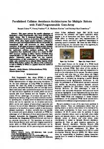
velocity vmax = 28cm/sec, and decision period ∆t = 0.5sec. The radius of the safety disk is R = vmax ∆t = 14cm. We tested the switching condition in the following two scenarios; snapshots from simulations of these scenarios appear in Fig. 12. Both scenarios involve an obstacle with lower bound on internal angles α = 70◦ . For the scenario in Fig. 12(a), we place the obstacle such that when the robot approaches the obstacle and the vertex with angle α is about to enter the safety disk, only one sensor detects an edge with lmin and the other edge barely misses the cone of observation of an adjacent sensor. This is the worst-case scenario for case 1 in Section 4.3. For the scenario in Fig. 12(b), we place the obstacle such that when the robot approaches the obstacle and the vertex with angle α is about to enter the safety disk, the vertex is in the gap of two adjacent sensors and both sensors detect an edge of the obstacle within lmin . This is the worst-case scenario for case 2 in Section 4.4. The snapshots in Fig. 12 show the moment when the switching condition becomes true and the robot stops. One observation is that, in both scenarios, the switching condition is correct: the obstacle does not enter the safety disk. Of course, this is expected. A more interesting observation is that, in both scenarios, the switching condition is tight (not unnecessarily conservative): the robot does not stop until the obstacle is about to enter the safety disk. The actual simulations leading to these snapshots can be viewed at https: //www.youtube.com/watch?v=bK-YnGgwjwU

Fig. 12. Snapshots from simulations showing the robot correctly stops to ensure no obstacles in the safety disk. The circle around the robot represents the safety disk. The red region represents the obstacle. The blue wedges represent the robot’s cones of observation. (a) Snapshot from scenario for case 1: a sensor detects an obstacle within lmin ; adjacent sensors do not. (b) Snapshot from scenario for case 2: two adjacent sensors detect an obstacle within lmin .

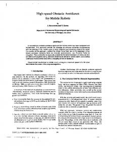
Fig. 13 shows how the switching threshold d1switch in case 1 depends on various parameters. Fig. 13(a) shows how d1switch decreases as α increases. It is

clear from the worst-case scenario of case 1 that when an obstacle with a sharper corner, i.e., a smaller α, touches the safety disk, the sensor detects its edge at a greater distance than one with a flatter corner, and this necessitates a larger d1switch . Fig. 13(b) shows how d1switch increases as β increases. Intuitively, a larger β means a larger gap between the cones of observation of two adjacent sensors, so the edge of the obstacle is detected at a larger distance when the vertex is at the boundary of the safety disk. Fig. 13(c) shows how d1switch decreases as lmin increases. This can be seen from the worst-case scenario: the edge of the obstacle that is not detected within lmin will make a smaller angle with the edge of the cone if lmin is larger, so the other edge is detected at a smaller distance. Fig. 13(d) shows how d1switch increases as R increases (note: it doesn’t matter whether the increase in R is due to an increase in vmax or ∆t). This directly reflects the fact that a robot with a larger safety disk needs to stop farther from obstacles.

Fig. 13. Graphs of d1switch as a function of various parameters, with graphs (a) and (b) on top, and graphs (c) and (d) on bottom. (a) d1switch as a function of α, with β = π/4, lmin = 80 and R = 14. (b) d1switch as a function of β, with α = π/2, lmin = 80 and R = 14. (c) d1switch as a function of lmin , with α = π/2, β = π/4, and R = 14. (d) d1switch as a function of R, with α = π/2, β = π/4, and lmin = 80.

6

Conclusions

In this paper, we have shown how it is possible to use the Simplex architecture, equipped with a sophisticated geometric-based switching condition, to ensure at runtime that mobile robots with limited field-of-view and limited sensing range do not collide with obstacles while navigating in an unknown environment. Future work includes extending our approach to take into account the size and shape of the robot, its braking power (instead of assuming immediate stop), and the minimum detection distance of the sensors. We will also consider more powerful baseline controllers. We also plan to develop algorithms that allow the robot to learn about its environment, enabling it to replace worst-case assumptions with more detailed information about obstacles it has encountered, allowing tighter switching conditions. The geometric analysis that we developed to derive and verify the switching condition can also be used as a basis for the design of collision-avoidance logic in navigation algorithms for mobile robots. Acknowledgments. This material is based upon work supported in part by AFOSR Grant FA9550-14-1-0261, NSF Grants IIS-1447549, CCF-0926190, CNS1421893, ONR Grant N00014-15-1-2208, and Artemis EMC2 Grant 3887039.

References 1. Alami, R., Krishna, K.M.: Provably safe motions strategies for mobile robots in dynamic domains. In: in Autonomous Navigation in Dynamic Environment: Models and Algorithms. in C. Laugier, R. Chatila (Eds.), Springer Tracts in Advanced Robotics (2007) 2. Bak, S., Manamcheri, K., Mitra, S., Caccamo, M.: Sandboxing controllers for cyberphysical systems. In: Proc. 2011 IEEE/ACM International Conference on CyberPhysical Systems ICCPS. pp. 3–12. IEEE Computer Society (2011) 3. Bouraine, S., Fraichard, T., Salhi, H.: Provably safe navigation for mobile robots with limited field-of-views in dynamic environments. Autonomous Robots 32(3), 267–283 (Apr 2012), https://hal.inria.fr/hal-00733913 4. Mitsch, S., Ghorbal, K., Platzer, A.: On provably safe obstacle avoidance for autonomous robotic ground vehicles. In: Newman, P., Fox, D., Hsu, D. (eds.) Robotics: Science and Systems (2013) 5. Pan, J., Zhang, L., Manocha, D.: Collision-free and smooth trajectory computation in cluttered environments. Int. J. Rob. Res. 31(10), 1155–1175 (Sep 2012), http: //dx.doi.org/10.1177/0278364912453186 6. QuickBot MOOC v2 (2014), http://o-botics.org/robots/quickbot/mooc/v2/ 7. Savkin, A.V., Wang, C.: A reactive algorithm for safe navigation of a wheeled mobile robot among moving obstacles. In: CCA. pp. 1567–1571. IEEE (2012), http:// dblp.uni-trier.de/db/conf/IEEEcca/IEEEcca2012.html#SavkinW12 8. Seto, D., Krogh, B., Sha, L., Chutinan, A.: The Simplex architecture for safe online control system upgrades. In: Proc. 1998 American Control Conference. vol. 6, pp. 3504–3508 (1998) 9. Sha, L.: Using simplicity to control complexity. IEEE Software 18(4), 20–28 (2001)