Collision Detection and Response for Interactive Editing of ... - CiteSeerX

Collision Detection and Response for Interactive Editing of Point-Sampled Models

Richard Keiser Diploma Thesis Winter 2002/2003 Computer Graphics Lab Departement of Computer Science ETH Zürich Prof. Dr. Markus Gross Mark Pauly

1Abstract

We introduce a framework for detecting self-collisions during interactive editing of point-sampled surfaces. Collision detection is based on a classification operator which computes whether a point is inside or outside of a model. This leads to a robust and efficient collision detection algorithm which exploits temporal coherence. Our framework allows to integrate any kind of bounding volume hierarchy (BVH). Using a generic BVH base class we have implemented axis-aligned bounding box (AABB) and oriented bounding box (OBB) trees. For improving performance we show how to approximate collision detection using clustering as a surface simplification approach. We also use this technique for efficiently creating a BVH with spheres as bounding volumes. We present different response possibilities for resolving a collision. Apart from responses which enforces a consistent topology instantaneously, we introduce a union operator which merges the penetrating part of a model with the rest and produces a sharp intersection curve. For creating a smooth transition between two areas we introduce a particle system as a blend tool.

III

IV

Eidgenossische ¨ Technische Hochschule Zurich ¨

´ ´ de Zurich Ecole polytechnique federale Politecnico federale di Zurigo Swiss Federal Institute of Technology Zurich

Diploma Thesis for Richard Keiser

Collision Detection and Response for Interactive Editing of Point-Sampled Models Introduction Methods for manipulating point-based 3D objects have been a focus of computer graphics research in recent years. Modern acquisition devices like laser range scanners create huge data sets, i.e. 3D point clouds, which are difficult to handle with conventional methods. The fundamental idea of point-based methods is to perform all operations directly on the point cloud without applying a surface reconstruction method to create a triangle mesh or spline surface. In the context of the Pointshop3D project, an environment has been developed that allows surface editing operations such as texturing and sculpting. The functionality of this system has recently been extended towards more general modeling operations such as boolean operations and free-form deformation. The goal of this thesis is to investigate aspects of self-intersection in this context.

Tasks • To become acquainted with point-based methods in computer graphics • To become acquainted with existing code of Pointshop3D • The following algorithms should be developed: • Methods for collision detection between rigid and deformable parts of the modeled surface • Approximation of collision detection using surface simplification • Method to create a sharp transition in case of a self-intersection using boolean operations, or a smooth transition using blending techniques • The above mentioned algorithms should be integrated into the existing deformation tool, putting particular emphasis on performance.

Comments A written report and an oral presentation of the results conclude the work. The thesis supervisor is Prof. Markus Gross, the thesis tutor is Mark Pauly, Institute of Scientific Computing. Beginning of thesis: 28.10.2002 Submission of thesis: 27.02.2003

V

VI

1Acknowledgments One never notices what has been done; one can only see what remains to be done. Marie Curie (1867-1934)

First of all I want to thank my mentor Mark Pauly. It is due to him that my diploma thesis was such an interesting and successful one, and it is also his fault that I will continue my work in point-based systems as a Ph.D. student. Further I want to thank all the people who came along with me during my years of study: my family for always supporting me, my friends which made this time such enjoyable, and my girlfriend Janine for her love. Thanks all, I will forget a lot of what I have learned in school, but I will never forget the time I spent with you.

VII

VIII

14Contents

1 Introduction . . . . . . . . . . . . . . . . . . . . . . . . . . . . . . . . . . . . . . . . . . . . . . . . . . . . . . . . . . . . . 1 1.1 Motivation . . . . . . . . . . . . . . . . . . . . . . . . . . . . . . . . . . . . . . . . . . . . . . . . . . . . . . . . . . 1 1.2 Previous Work . . . . . . . . . . . . . . . . . . . . . . . . . . . . . . . . . . . . . . . . . . . . . . . . . . . . . . . 2 1.3 Overview . . . . . . . . . . . . . . . . . . . . . . . . . . . . . . . . . . . . . . . . . . . . . . . . . . . . . . . . . . . 3 2 A Survey of 3D Collision Detection . . . . . . . . . . . . . . . . . . . . . . . . . . . . . . . . . . . . . . . . . . 5 2.1 Introduction . . . . . . . . . . . . . . . . . . . . . . . . . . . . . . . . . . . . . . . . . . . . . . . . . . . . . . . . . 5 2.2 Bounding Volume Hierarchies . . . . . . . . . . . . . . . . . . . . . . . . . . . . . . . . . . . . . . . . . . 6 2.2.1 Spatial Partitioning Representations . . . . . . . . . . . . . . . . . . . . . . . . . . . . . . . 6 2.2.2 Object Partitioning Representations . . . . . . . . . . . . . . . . . . . . . . . . . . . . . . . . 6 3 Application: Pointshop3D . . . . . . . . . . . . . . . . . . . . . . . . . . . . . . . . . . . . . . . . . . . . . . . . . 9 3.1 Introduction . . . . . . . . . . . . . . . . . . . . . . . . . . . . . . . . . . . . . . . . . . . . . . . . . . . . . . . . . 9 3.2 Deformation Tool . . . . . . . . . . . . . . . . . . . . . . . . . . . . . . . . . . . . . . . . . . . . . . . . . . . . 9 3.3 Collision Detection in Pointshop3D . . . . . . . . . . . . . . . . . . . . . . . . . . . . . . . . . . . . . 11 4 Collision Detection with Point-Sampled Models . . . . . . . . . . . . . . . . . . . . . . . . . . . . . . 13 4.1 Inside/Outside Classification . . . . . . . . . . . . . . . . . . . . . . . . . . . . . . . . . . . . . . . . . . . 13 4.2 Collision Definition . . . . . . . . . . . . . . . . . . . . . . . . . . . . . . . . . . . . . . . . . . . . . . . . . . 15 5 k-d Tree . . . . . . . . . . . . . . . . . . . . . . . . . . . . . . . . . . . . . . . . . . . . . . . . . . . . . . . . . . . . . . . 17 5.1 Introduction . . . . . . . . . . . . . . . . . . . . . . . . . . . . . . . . . . . . . . . . . . . . . . . . . . . . . . . . 17 5.2 Requirements & Goals . . . . . . . . . . . . . . . . . . . . . . . . . . . . . . . . . . . . . . . . . . . . . . . 18 5.3 The k-d Tree Algorithm . . . . . . . . . . . . . . . . . . . . . . . . . . . . . . . . . . . . . . . . . . . . . . 18 5.3.1 Creating the k-d Tree . . . . . . . . . . . . . . . . . . . . . . . . . . . . . . . . . . . . . . . . . . 18 5.3.2 Node Structure . . . . . . . . . . . . . . . . . . . . . . . . . . . . . . . . . . . . . . . . . . . . . . . 20 5.3.3 Querying the k-d Tree . . . . . . . . . . . . . . . . . . . . . . . . . . . . . . . . . . . . . . . . . . 20 5.3.4 Other Query Algorithm Trials . . . . . . . . . . . . . . . . . . . . . . . . . . . . . . . . . . . . 22 5.3.5 Range Searching . . . . . . . . . . . . . . . . . . . . . . . . . . . . . . . . . . . . . . . . . . . . . . 23 5.4 Test Application . . . . . . . . . . . . . . . . . . . . . . . . . . . . . . . . . . . . . . . . . . . . . . . . . . . . 23 5.5 Performance . . . . . . . . . . . . . . . . . . . . . . . . . . . . . . . . . . . . . . . . . . . . . . . . . . . . . . . . 24 5.6 Summary & Discussion . . . . . . . . . . . . . . . . . . . . . . . . . . . . . . . . . . . . . . . . . . . . . . . 28 6 Collision Detection Algorithms . . . . . . . . . . . . . . . . . . . . . . . . . . . . . . . . . . . . . . . . . . . . 29 6.1 A Simple Algorithm . . . . . . . . . . . . . . . . . . . . . . . . . . . . . . . . . . . . . . . . . . . . . . . . . 29 6.1.1 Problems and Heuristic Solutions . . . . . . . . . . . . . . . . . . . . . . . . . . . . . . . . . 29 6.1.2 Spatial Coherence . . . . . . . . . . . . . . . . . . . . . . . . . . . . . . . . . . . . . . . . . . . . . 31 6.2 An Efficient Algorithm Using Temporal Coherence . . . . . . . . . . . . . . . . . . . . . . . . 32 6.3 A Robust Algorithm . . . . . . . . . . . . . . . . . . . . . . . . . . . . . . . . . . . . . . . . . . . . . . . . . 33 6.3.1 Using Temporal Coherence . . . . . . . . . . . . . . . . . . . . . . . . . . . . . . . . . . . . . 35 6.4 Performance . . . . . . . . . . . . . . . . . . . . . . . . . . . . . . . . . . . . . . . . . . . . . . . . . . . . . . . . 35 6.5 Summary & Discussion . . . . . . . . . . . . . . . . . . . . . . . . . . . . . . . . . . . . . . . . . . . . . . . 38 7 Bounding Volume Hierarchies . . . . . . . . . . . . . . . . . . . . . . . . . . . . . . . . . . . . . . . . . . . . 39 7.1 Introduction . . . . . . . . . . . . . . . . . . . . . . . . . . . . . . . . . . . . . . . . . . . . . . . . . . . . . . . . 39 7.2 Base Class for BVHs . . . . . . . . . . . . . . . . . . . . . . . . . . . . . . . . . . . . . . . . . . . . . . . . . 40

IX

7.3

7.4

7.2.1 BVH Interface . . . . . . . . . . . . . . . . . . . . . . . . . . . . . . . . . . . . . . . . . . . . . . . . 40 A Bounding Box Hierarchy Base Class . . . . . . . . . . . . . . . . . . . . . . . . . . . . . . . . . . 41 7.3.1 Disadvantages of Virtual Methods . . . . . . . . . . . . . . . . . . . . . . . . . . . . . . . . 41 7.3.2 Using C++ Templates . . . . . . . . . . . . . . . . . . . . . . . . . . . . . . . . . . . . . . . . . 41 7.3.3 BBH Interface . . . . . . . . . . . . . . . . . . . . . . . . . . . . . . . . . . . . . . . . . . . . . . . . 41 7.3.4 Box Interface . . . . . . . . . . . . . . . . . . . . . . . . . . . . . . . . . . . . . . . . . . . . . . . . 42 7.3.5 Example Box Structure . . . . . . . . . . . . . . . . . . . . . . . . . . . . . . . . . . . . . . . . . 43 7.3.6 Building the Tree . . . . . . . . . . . . . . . . . . . . . . . . . . . . . . . . . . . . . . . . . . . . . 43 7.3.7 Intersection Test . . . . . . . . . . . . . . . . . . . . . . . . . . . . . . . . . . . . . . . . . . . . . . 44 Summary . . . . . . . . . . . . . . . . . . . . . . . . . . . . . . . . . . . . . . . . . . . . . . . . . . . . . . . . . . 45

8 AABB & OBB Trees . . . . . . . . . . . . . . . . . . . . . . . . . . . . . . . . . . . . . . . . . . . . . . . . . . . . 47 8.1 AABB Tree . . . . . . . . . . . . . . . . . . . . . . . . . . . . . . . . . . . . . . . . . . . . . . . . . . . . . . . . 47 8.1.1 Building the AABB Tree . . . . . . . . . . . . . . . . . . . . . . . . . . . . . . . . . . . . . . . . 47 8.1.1.1 Time Complexity for Building the AABB Tree . . . . . . . . . . . . . . . . . . 48 8.1.2 Intersection Tests . . . . . . . . . . . . . . . . . . . . . . . . . . . . . . . . . . . . . . . . . . . . . 48 8.1.2.1 AABB/Surfel . . . . . . . . . . . . . . . . . . . . . . . . . . . . . . . . . . . . . . . . . . . . 48 8.1.2.2 AABB/AABB . . . . . . . . . . . . . . . . . . . . . . . . . . . . . . . . . . . . . . . . . . . . 48 8.2 OBB Tree . . . . . . . . . . . . . . . . . . . . . . . . . . . . . . . . . . . . . . . . . . . . . . . . . . . . . . . . . 51 8.2.1 Building the OBB Tree . . . . . . . . . . . . . . . . . . . . . . . . . . . . . . . . . . . . . . . . . 52 8.2.2 Intersection Tests . . . . . . . . . . . . . . . . . . . . . . . . . . . . . . . . . . . . . . . . . . . . . 52 8.2.2.1 OBB/Surfel . . . . . . . . . . . . . . . . . . . . . . . . . . . . . . . . . . . . . . . . . . . . . 52 8.2.2.2 OBB/AABB . . . . . . . . . . . . . . . . . . . . . . . . . . . . . . . . . . . . . . . . . . . . . 53 8.3 Updating . . . . . . . . . . . . . . . . . . . . . . . . . . . . . . . . . . . . . . . . . . . . . . . . . . . . . . . . . . 54 8.3.1 Updating of AABBs . . . . . . . . . . . . . . . . . . . . . . . . . . . . . . . . . . . . . . . . . . . . 54 8.3.2 Insertion/Deletion of Surfels . . . . . . . . . . . . . . . . . . . . . . . . . . . . . . . . . . . . . 56 8.3.3 Recreation on Idle . . . . . . . . . . . . . . . . . . . . . . . . . . . . . . . . . . . . . . . . . . . . 57 8.4 Concave Collisions . . . . . . . . . . . . . . . . . . . . . . . . . . . . . . . . . . . . . . . . . . . . . . . . . . 57 8.5 Performance Comparison of AABB/OBB . . . . . . . . . . . . . . . . . . . . . . . . . . . . . . . . 58 8.5.1 Cost Equation . . . . . . . . . . . . . . . . . . . . . . . . . . . . . . . . . . . . . . . . . . . . . . . . 58 8.5.2 BVH for Zero Region only . . . . . . . . . . . . . . . . . . . . . . . . . . . . . . . . . . . . . . 58 8.5.3 BVH for Zero and Deformable Region . . . . . . . . . . . . . . . . . . . . . . . . . . . . . 60 8.5.4 Concave Collisions . . . . . . . . . . . . . . . . . . . . . . . . . . . . . . . . . . . . . . . . . . . . 60 8.6 Summary & Discussion . . . . . . . . . . . . . . . . . . . . . . . . . . . . . . . . . . . . . . . . . . . . . . 61 9 Surface Simplification & Sphere Cluster Tree . . . . . . . . . . . . . . . . . . . . . . . . . . . . . . . 63 9.1 Introduction . . . . . . . . . . . . . . . . . . . . . . . . . . . . . . . . . . . . . . . . . . . . . . . . . . . . . . . . 63 9.2 Surface Simplification . . . . . . . . . . . . . . . . . . . . . . . . . . . . . . . . . . . . . . . . . . . . . . . 64 9.2.1 Clustering by Region-growing . . . . . . . . . . . . . . . . . . . . . . . . . . . . . . . . . . . 64 9.2.2 Hierarchical Clustering . . . . . . . . . . . . . . . . . . . . . . . . . . . . . . . . . . . . . . . . 64 9.3 Approximation of Collision Detection . . . . . . . . . . . . . . . . . . . . . . . . . . . . . . . . . . . 65 9.3.1 Performance . . . . . . . . . . . . . . . . . . . . . . . . . . . . . . . . . . . . . . . . . . . . . . . . . 65 9.4 Building a Sphere Cluster Tree . . . . . . . . . . . . . . . . . . . . . . . . . . . . . . . . . . . . . . . . . 67 9.4.1 Sphere Tree Construction Using Hierarchical Clustering . . . . . . . . . . . . . . 67 9.4.2 Sphere Tree Construction Using Clustering by Region-growing . . . . . . . . . 68 9.4.3 Intersection Tests . . . . . . . . . . . . . . . . . . . . . . . . . . . . . . . . . . . . . . . . . . . . . 69 9.4.4 Performance . . . . . . . . . . . . . . . . . . . . . . . . . . . . . . . . . . . . . . . . . . . . . . . . . 69 9.5 Summary & Discussion . . . . . . . . . . . . . . . . . . . . . . . . . . . . . . . . . . . . . . . . . . . . . . 71 10 Collision Detection Results . . . . . . . . . . . . . . . . . . . . . . . . . . . . . . . . . . . . . . . . . . . . . . . 73 10.1 Robustness . . . . . . . . . . . . . . . . . . . . . . . . . . . . . . . . . . . . . . . . . . . . . . . . . . . . . . . . 73

X

10.1.1 Robustness Issues for BVHs . . . . . . . . . . . . . . . . . . . . . . . . . . . . . . . . . . . . . 73 10.2 Performance . . . . . . . . . . . . . . . . . . . . . . . . . . . . . . . . . . . . . . . . . . . . . . . . . . . . . . . . 74 10.2.1 Performance Tests . . . . . . . . . . . . . . . . . . . . . . . . . . . . . . . . . . . . . . . . . . . . . 74 10.2.2 Collision Detection Performance . . . . . . . . . . . . . . . . . . . . . . . . . . . . . . . . . 75 10.2.3 Preprocessing Performance . . . . . . . . . . . . . . . . . . . . . . . . . . . . . . . . . . . . . 76 10.3 Summary & Discussion . . . . . . . . . . . . . . . . . . . . . . . . . . . . . . . . . . . . . . . . . . . . . . . 78 11 Collision Response . . . . . . . . . . . . . . . . . . . . . . . . . . . . . . . . . . . . . . . . . . . . . . . . . . . . . . 79 11.1 Introduction . . . . . . . . . . . . . . . . . . . . . . . . . . . . . . . . . . . . . . . . . . . . . . . . . . . . . . . . 79 11.2 Response for Rigid Deformable Region . . . . . . . . . . . . . . . . . . . . . . . . . . . . . . . . . . 80 11.3 Merging . . . . . . . . . . . . . . . . . . . . . . . . . . . . . . . . . . . . . . . . . . . . . . . . . . . . . . . . . . . 81 11.4 Summary & Discussion . . . . . . . . . . . . . . . . . . . . . . . . . . . . . . . . . . . . . . . . . . . . . . . 83 12 Particle System as a Blend Tool . . . . . . . . . . . . . . . . . . . . . . . . . . . . . . . . . . . . . . . . . . . . 85 12.1 Introduction . . . . . . . . . . . . . . . . . . . . . . . . . . . . . . . . . . . . . . . . . . . . . . . . . . . . . . . . 85 12.2 Oriented Particle System . . . . . . . . . . . . . . . . . . . . . . . . . . . . . . . . . . . . . . . . . . . . . . 86 12.2.1 Oriented Particles . . . . . . . . . . . . . . . . . . . . . . . . . . . . . . . . . . . . . . . . . . . . . 86 12.2.2 Surface Potentials . . . . . . . . . . . . . . . . . . . . . . . . . . . . . . . . . . . . . . . . . . . . . 86 12.2.3 Dynamics . . . . . . . . . . . . . . . . . . . . . . . . . . . . . . . . . . . . . . . . . . . . . . . . . . . . 86 12.2.4 Repulsion Force . . . . . . . . . . . . . . . . . . . . . . . . . . . . . . . . . . . . . . . . . . . . . . 88 12.2.5 Weighting Function . . . . . . . . . . . . . . . . . . . . . . . . . . . . . . . . . . . . . . . . . . . . 89 12.2.6 Equation of Motion . . . . . . . . . . . . . . . . . . . . . . . . . . . . . . . . . . . . . . . . . . . . 91 12.2.7 Integration . . . . . . . . . . . . . . . . . . . . . . . . . . . . . . . . . . . . . . . . . . . . . . . . . . . 91 12.3 Blending - Implementation Details . . . . . . . . . . . . . . . . . . . . . . . . . . . . . . . . . . . . . . 92 12.3.1 Initialization . . . . . . . . . . . . . . . . . . . . . . . . . . . . . . . . . . . . . . . . . . . . . . . . . 92 12.3.2 Region Scaling . . . . . . . . . . . . . . . . . . . . . . . . . . . . . . . . . . . . . . . . . . . . . . . 92 12.3.3 Neighborhood Computation . . . . . . . . . . . . . . . . . . . . . . . . . . . . . . . . . . . . . 93 12.3.4 Starting the Particle Simulation . . . . . . . . . . . . . . . . . . . . . . . . . . . . . . . . . . 94 12.3.5 Velocity Control . . . . . . . . . . . . . . . . . . . . . . . . . . . . . . . . . . . . . . . . . . . . . . 94 12.3.6 Blending Along the Normal Vector . . . . . . . . . . . . . . . . . . . . . . . . . . . . . . . . 95 12.3.7 Local Adaptive Repulsion . . . . . . . . . . . . . . . . . . . . . . . . . . . . . . . . . . . . . . . 96 12.4 Further Applications . . . . . . . . . . . . . . . . . . . . . . . . . . . . . . . . . . . . . . . . . . . . . . . . . 96 12.4.1 Blending for Boolean Operations . . . . . . . . . . . . . . . . . . . . . . . . . . . . . . . . . 96 12.4.2 Hole-Filling . . . . . . . . . . . . . . . . . . . . . . . . . . . . . . . . . . . . . . . . . . . . . . . . . . 98 12.5 Summary and Discussion . . . . . . . . . . . . . . . . . . . . . . . . . . . . . . . . . . . . . . . . . . . . . 98 13 Conclusions & Future Work . . . . . . . . . . . . . . . . . . . . . . . . . . . . . . . . . . . . . . . . . . . . . 101 A References . . . . . . . . . . . . . . . . . . . . . . . . . . . . . . . . . . . . . . . . . . . . . . . . . . . . . . . . . . . . 105

XI

XII

1 1Introduction

1.1 Motivation The problem of fast and accurate collision detection (also known as interference detection or contact determination) between geometric objects is fundamental in CAD/CAM, robotics, manufacturing, computer graphics, animation and computer-simulated environments (e.g. virtual environments). Geometric models can be described by a number of different surface representations including polygonal meshes, splines, algebraic surfaces or point clouds. In our case the object is represented by an unstructured cloud of points, where each point is stored with its normal vector which is oriented such that it points outward the surface. As opposed to triangle meshes, point samples do not store information about local surface connectivity, which makes them particularly suitable for large graphics data sets. In such complex models the triangle size is decreasing to pixel resolution, which may cause substantial performance overheads during scan conversion. Point-based rendering [52, 57] is an alternative rendering technique to conventional polygon based rendering that avoids these overheads by using simpler rendering primitives. Furthermore, there is no connectivity graph which must be kept consistent during interactive modifications of the geometry. Point-based models are a natural representation for data captured by laser range scanners and similar devices. Our application for collision detection is an editor for point-based models called Pointshop3D. With Pointshop3D the shape and appearance of such models can be edited interactively. Recently, Pointshop3D was extended to supply interactive deformation of a model. During deformation, parts of the model may self-intersect. To keep the surface in a consistent state we have to detect and resolve such self-collisions. Because this is done during the interactive editing process, we have to solve the collision detection problem in real-time whereby speed is the most important factor. This is a challenging problem because in many applications collision detection is considered as a major computational bottleneck. The purpose of collision detection is to give an appropriate response when a collision has occurred. This can e.g. be a simple message or a complex reaction based on physical laws. In our application, we want to support the user with different suitable response possibilities. We can characterize our collision detection algorithm as follows: • Model complexity: The input models may consist of many hundreds of thousands of points. 1

2

1. INTRODUCTION

• Representation: The model is sampled irregularly. We have neither topology nor connectivity information. • Interaction: The model may undergo any deformation. The collision detection and response algorithms should not affect the interactive deformation until a collision occurs. Further, collision detection should not affect the speed of the deformation (frame rate) significantly. • Dynamic resampling: During the deformation the deformable part of the model might be resampled. Therefore our collision detection algorithm needs to handle the insertion and deletion of points. • Collision detection: Multiple contacts between the deformable and the rigid part of the model may occur. The algorithm has to detect these contacts accurately. • Collision response: The collision detection algorithm has to provide the information for a collision response. This means in particular that all intersecting surfels have to be reported. After collision response the surface has to be in a consistent state. We introduce efficient algorithms to accurately detect collisions during the interactive deformation of point-sampled models. Further we present several response possibilities which are suitable for Pointshop3D to support the user during editing. Our main contributions are: • An algorithm that classifies a point as inside or outside of a point-sampled model. • Adapting existing bounding volume hierarchy techniques for collision detection to pointsampled models, as e.g. axis-aligned bounding box (AABB) and oriented bounding box (OBB) trees. • A new robust and efficient collision detection algorithm exploiting temporal coherence which comes along without a bounding volume hierarchy. • Approximation of collision detection using model simplification methods. • Applying the simplification techniques for guiding the creation of a sphere bounding volume hierarchy which we call a sphere cluster tree. • A union operator for joining the self-colliding part with the rest of the model, which produces a sharp intersection curve. • A blend tool using a particle system for creating a smooth transition between the two joined areas. The blend tool can also be used for other applications, e.g. after a boolean operation between two or more models has been applied, or for filling holes in models.

1.2 Previous Work The importance of collision detection can be recognized at the rich literature which deals with the subject (see also the survey in Chapter 2). Nowadays, many collision detection algorithms use some kind of bounding volume hierarchy. Popular choices for bounding volumes are spheres [32, 31, 30, 49], axis-aligned bounding boxes [6, 29, 8], oriented bounding boxes [26, 25] and discrete orientation polytopes (k-dops) [35, 34]. An incremental collision detection algorithm for hierarchical data structures which makes use of temporal coherence was presented by Li and Chen [40]. Only little work has been done for updating bounding volume hierarchies. Van den Bergen [68] showed how to efficiently merge axis-aligned bounding boxes for a bottom-up update approach. Larsson and Akenine-Möller [37] improved updating by using a hybrid updating approach which combines the advantages of top-down and bottom-up update methods.

1.3 OVERVIEW

3

Another approach for a collision detection algorithm is to use Voronoi diagrams [13, 41, 42] to keep track of the closest features between pairs of objects. A “sweep-and-prune” technique [13] is used to reduce the pairs of objects that need to be considered for collision. The disadvantage of this technique is that the objects need to be convex. Ponamgi et al. [53] have generalized this work to include non-convex objects. The “sweep-and-prune” technique has been further improved by Chung [12] replacing the “closest pairs of features” algorithm with a “separating vector” algorithm, which quickly finds a separating plane between convex polytopes if they do not intersect. Nearest neighbor and distance queries are very important for point-based systems in general and for collision detection with point-sampled models in particular. Bentley [7] introduced a binary search tree called k-d tree for efficient nearest neighbor queries in a static environment. Many improvements have been presented since then [21, 61, 8]. Arya et al. [3] use an incremental distance calculation approach to speed up the k-d algorithm. Their library ANN is freely available on the web. A spatial data structure which is also efficient for range queries when the position of data points changes or when data points are inserted and deleted was presented by Heckbert [28]. He uses a grid which is (re-)computed according to the density of the points. Particle systems are often used for simulating physical systems and are also applied in computer graphics [56, 60]. Szeliski and Tonnesen [64, 65, 66, 67] used oriented particles for surface modeling. They devised new interaction potentials which favor locally planar or spherical arrangement. Witkin and Heckbert [71] use particles to sample and control implicit surfaces. They presented an adaptive repulsion scheme in which particles may fission or die. Point sample rendering became popular with the pioneering work of Levoy and Whitted [39]. Levin [38] has introduced a new point-based surface representation called moving least squares (MLS) surfaces. Based on this representation, Alexa et al. [1] implemented a high-quality rendering algorithm for point set surfaces. Pointshop3D was presented by Zwicker et al. [72] as an interactive system for point-based surface editing. Pauly et al. [51] improved interactive modeling, such as interactive deformation of a model, using a multiresolution approach.

1.3 Overview We start by giving an overview over the state of the art in collision detection in Chapter 2, where we especially concentrate on bounding volume hierarchies. Our collision detection framework is part of a deformation tool for Pointshop3D. We give a brief introduction to Pointshop3D in Chapter 3 where we also describe the deformation tool. We then discuss the tasks of our collision detection algorithms within Pointshop3D and some of our design choices. Point-sampled models have no explicitly defined surface. Therefore it is not clear what a collision between point clouds is. We base our collision definition on an inside/outside classification. In Chapter 4 we derive an inside/outside definition which can be used directly as an algorithm for the inside/outside test. For the inside/outside classification we make extensive use of nearest neighbor queries. Therefore we have implemented a k-d tree as a spatial data structure which is very efficient and suited to our needs. This is described in Chapter 5. Using the inside/outside test we give an algorithm for collision detection in Chapter 6. We develop this algorithm further to use spatial and temporal coherence. Finally, we present a collision detection algorithm which is both very robust and efficient.

4

1. INTRODUCTION

Bounding volume hierarchies (BVHs) are often used for collision detection. In Chapter 7 we show how to adapt BVHs to point-sampled models. Further we present our framework for integrating different bounding volumes (BVs) with little effort. Implementation details of two of the most used BVs, namely axis-aligned bounding boxes (AABBs) and oriented bounding boxes (OBBs), are given in Chapter 8. Simplification methods are widely used to improve the performance of algorithms. We present two such methods based on clustering and show how to approximate collision detection in Chapter 9. Further we use these methods for efficiently creating a tight fitting BVH using spheres as BVs. We call this BVH a sphere cluster tree. In Chapter 10 we compare the performance and robustness of different collision detection algorithms. We discuss the advantages and drawbacks of collision detection algorithms using and not using BVHs respectively. A collision can be resolved in several ways. In Chapter 11 we discuss and present possible responses which are suitable for our application. Further we present a merging operator which joins the intersecting part with the rest of the model using again the inside/outside classification. The merging operator mentioned before produces sharp creases between two merged regions. However, sometimes we wish to have a smooth transition between both areas. Therefore we introduce a particle system as a blend tool in Chapter 12. Finally, we summarize our results and conclude with extensions and future work in the last chapter.

2 2A Survey of 3D Collision Detection

Fast and robust 3D collision detection algorithms are required in many applications and are often considered as the main bottleneck. Therefore a lot of literature about collision detection exists. In this chapter, we have a look at the state of the art in collision detection for geometric models where we concentrate especially on bounding volume hierarchies. Other surveys can be found e.g. in [33, 43].

2.1 Introduction Collision detection methods are usually split into three categories: • Static collision detection (discrete methods): The objects motions are sampled and the objects interpenetrations are statically checked. This is much easier and more efficient than the dynamic approaches described below, but as a result collisions may be missed (tunneling effect). • Pseudo-dynamic collision detection (discrete methods): For solving the problem described above one can use an adaptive time-step and predictive methods. This may work fine in offline applications, but it is not suitable in interactive applications when a relatively high and constant frame-rate is required. • Dynamic collision detection (continuos methods): Dynamic methods determine the time of first contact between objects. While more suitable to robust interactive dynamics simulations, these methods are usually much slower than discrete methods. In dynamic environments when objects rotate and translate and queries are executed repeatedly on the same models at successive time steps, the geometric relationship may only differ slightly from that of the previous step. Algorithms which use this property are said to exploit temporal coherence. Similar to that, if a model is deformable and deformations between time steps are small, an algorithm may exploit this kind of coherence as well. If the spatial relationship of the primitives of an object is used for improving the performance of collision queries then we say that an algorithm exploits spatial coherence. Another possible classification criterion for collision detection strategies is whether they require that an object is convex or not. Algorithms which assume convexity are in general more efficient than those which allow also non-convex objects. Lin et al. [42] showed that intersec5

6

2. A SURVEY OF 3D COLLISION DETECTION

tion detection for two convex polyhedra can be done in linear time in the worst case. The proof is by reduction to linear programming, which is solvable in linear time for any fixed number of variables. The idea is that the convex hulls of two disjoint point sets can be separated by a plane. A plane is described by three parameters which are considered as variables. For each vertex a linear inequality is attached which describes that the point is on one side of the plane. It is even possible to drop the complexity of collision detection to O  log n ˜ log m by preprocessing the convex polyhedra, where m and n are the number of vertices of the two polyhedra [17]. However, a practical disadvantage of the algorithm is that it reports only one collision point even if multiple parts of the objects collide which may be insufficient information for collision response. Collision detection is often divided into two phases: the task of rapidly eliminating most primitives which surely not belong to a collision is referred to as broad-phase collision detection. The task of finding out precisely which of the remaining primitives intersect with others is called narrow-phase collision detection [63].

2.2 Bounding Volume Hierarchies Bounding volume hierarchies (BVHs) are a means to reduce the number of primitives which have to be tested for intersection. They are applied in almost every state of the art collision detection algorithm for non-convex objects. BVHs are used to approximate the objects with simplified bounding volumes or to decompose the space they occupy. The advantage is that collision can often be ruled out at the first levels of the hierarchy. In the next sections, we have a look at different space and object partitioning representations. 2.2.1 Spatial Partitioning Representations Spatial partitioning algorithms divide the space into cells. The cells are divided again until a leaf cell contains d k primitives, for some threshold k. The advantage is that one needs to check for contact only those pairs of objects that are in the same or nearby cells of the decomposition. Examples of spatial partitioning representations are octrees [27] or octree-like structures [5], binary space partition (BSP) trees [46], brep-indices [9] and regular grids [22]. Octrees and BSP trees are the most widely used. Octrees recursively partition cubes into octants, and BSPtrees recursively cut the space by hyperplanes. BSP-trees can be considered a crossing between octrees and boundary representations because the partitioning is not restricted to be axisaligned. This is advantageous if the model is transformed because the transformation can be simply applied to each hyperplane without rebuilding the whole representation. A k-d tree is a special kind of a BSP tree. The splitting planes of a k-d tree are always chosen orthogonal to the coordinate axes. A description of our k-d tree implementation is given in Chapter 5. 2.2.2 Object Partitioning Representations A bounding volume hierarchy which partitions the object can be seen as a level-of-detail representation of an object. The root approximates the object only roughly. At each level down the hierarchy the approximation fits the object more tightly. There exists a large variety of bounding volume types in the literature, each of them having their own advantages and weaknesses. Several criteria are considered in choosing a suitable bounding volume (BV):

2.2 BOUNDING VOLUME HIERARCHIES

7

• efficient intersection detection: How efficient can an intersection be detected between two bounding volumes or between a primitive and a volume. • tight fitting: How well is the object contained in a BV with minimum empty space. • efficient updating: How efficient is updating the bounding volume if the positions of the primitives change, the positions or orientations of the objects change or primitives are added/removed from the hierarchy. • compact description: How many values are required for describing a BV. • efficient building: How efficient is computing a BV. This is usually done in a preprocessing step, but might be also necessary for updating. • dependencies: Does the BV depends on the environment, e.g. axis-dependency, scaling, etc. Below, we shortly describe the most popular bounding volumes: Spheres have the advantage that they are rotation invariant and that distance checking between two spheres can simply be done by comparing the distance of their centers with the sum of their radii. Therefore, a sphere can be compactly described by its center coordinates and the radius. Hubbard [32] showed how to place the spheres using medial-axis surfaces such that a tight fitting bounding volume arises, but this requires complex geometrical calculations. Furthermore, spheres do not bound elongated objects tightly. Axis-aligned bounding boxes (AABBs) can be described by their center coordinates and the three axes extents. An intersection test can be efficiently performed by verifying the coordinate overlap along all the axes. AABBs are easy to build and are suitable for update. Disadvantages are that they often do not fit the object very tightly, particularly for objects which are elongated in diagonal directions. Further, AABBs are not rotation invariant. An oriented bounding box (OBB) is a rectangular bounding box with arbitrary orientation in 3-space. It can be described with its center coordinates, the three axes extents and a rotation matrix. The rotation matrix defines the transformation from the canonical coordinate system to the OBB coordinate system which is spanned by the three axes. Gottschalk et al. [26] describe in how to construct a tight fitting oriented bounding box and how to efficiently test two OBBs for intersection. Because OBBs generally enclose the object more tightly than AABBs or spheres, fewer intersection tests are necessary on average. Further are OBBs rotation invariant. However, because the box can have any orientation the intersection test and also updating of the box is more expensive. Discrete orientation polytopes (k-dops) [34] attain a compromise between the relatively poor tightness of bounding spheres and AABBs, and the relatively high costs of overlap tests and updates associated with OBBs and convex hulls. k-dops are convex polytopes whose faces are determined by parallel slabs whose outward normals come from a small fixed set of k orientations. A k-dop can be described by the k values for the k axes. Their intersection test is similar to that of the AABBs and faster than that of OBBs. k-dops are not rotation invariant and expensive to update.

8

2. A SURVEY OF 3D COLLISION DETECTION

3 3Application: Pointshop3D

We implemented our work as an extension of Pointshop3D. In this chapter, we shortly describe Pointshop3D. We refer to [72] for further information. Pointshop3D can be freely downloaded at www.pointshop3d.com. New features described in this paper may be available soon.

3.1 Introduction Pointshop3D is an editor for point-sampled models. It is purely founded on 3D points as powerful and versatile 3D image primitives. It provides a set of tools to edit geometry and appearance of the model and stores the changed object again as a point-sampled model. The interaction techniques include e.g. cleaning, texturing, sculpting, carving, filtering and resampling. The functionality of Pointshop3D can be extended by plug-ins and tools at runtime. Recently, Pointshop3D was enhanced with a deformation tool for the interactive deformation of models. More information on how to write plug-ins and tools can be found on the Pointshop3D home page. In Pointshop3D interactive parametrization and dynamic resampling is used for supplying the editing operations. Parametrization is user triggered by specifying a set of feature points using an algorithm which computes the minimum distortion parametrization of point-based objects. Dynamic resampling is used to adapt the number of samples for properly representing fine geometric or appearance details [72].

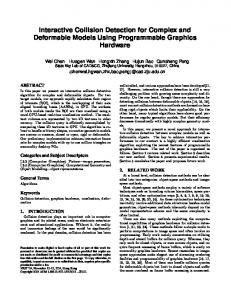
3.2 Deformation Tool The deformation tool developed by Pauly et al. [51] enables interactive free-form deformation of models in Pointshop3D. Both translation and rotation are supported. The region which is deformed, respectively rigid, can be chosen using the selection tool. An example is shown in Fig. 3.1 (a). The blue region is the so-called zero-region F 0 and the red region is called oneregion F 1 . The white and red region build the deformable region, while the zero-region is also called the rigid region. With F 0 and F 1 a continuous tensor-field can be computed which defines a transformation for each point in space based on a continuously varying scale parameter s  > 0 1 @ . Points 9

10

3. APPLICATION: POINTSHOP3D

(a) zero- and one-region

(b) after deformation

(c) smooth blending function

(d) quadratic blending function

Figure 3.1:

Zero- and deformable region with different blending functions.

within F 0 will not be displaced at all (s = 0), while points within F 1 will experience the maximum displacement (s = 1). All other points have to be displaced such that a smooth transition between F 0 and F 1 is created. For that, we compute for each point p its minimum distance d 0  p to the zero-region and its minimum distance d 1  p to the one-region. The scale parameter s is then computed as d0  p s = E §© ---------------------------------·¹ , d0  p + d1  p

(3.1)

where E is a blending function. A possible choice for the blending function is E  x =  x 2 – 1 2 , satisfying E  0 = 1 , E  1 = 0 and Ec  0 = Ec  1 = 0 . The new position pc for p is then determined as pc = F  p s where F is a deformation function. For translation we define F T  p s = p + s ˜ t with t the translation vector and F R  p s = R  a s ˜ D ˜ p for rotation, where R  a s ˜ D is the matrix that specifies a rotation around axis a with angle D . The deformation function composed of a translation and a rotation is then given as F  p s = F T  p s + F R  p s . In Fig. 3.1 (c) and (d) different blending functions are shown. In (c) we used a smooth and in (d) a quadratic blending function.

3.3 COLLISION DETECTION IN POINTSHOP3D

11

During deformation strong distortions in the distribution of sample points may occur leading to an insufficient local sampling density. Therefore new sample points should be inserted into the model such that a uniform distribution is maintained. The first fundamental form at each sample point is used as a measure of the local stretching [16]. If the distortion becomes too strong, new samples are inserted. Insertion is done by splitting a surfel into two new samples which are positioned along the axis of greatest stretch. The property values of the new samples are computed using an interpolation filter, while for achieving a uniform distribution a relaxation filter is used. For details we refer to [51].

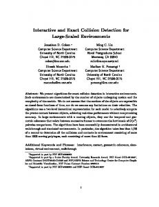
3.3 Collision Detection in Pointshop3D To achieve topological consistency during the deformation we have to detect self-intersections of the deformed model. As already mentioned speed is an important factor for collision detection because interactivity should be preserved. We divide collision detection into detecting self-intersections between the deformable region and the rigid region, and between the deformable region and itself. As we will see later, the former can be performed very efficiently while the latter is computationally very expensive. We therefore assume that intersections may occur only between the deformable and the zero region. Further, we provide only static collision detection checks. This means that we do a collision detection after a transformation step is performed and before the transformed model is rendered. Therefore the transformation should be only small per step because otherwise collisions which happen “between” the transformation may not be detected. This might be especially the case during rotations. However, static tests have the advantage that only the state before and after the transformation is decisive whether there is a collision or not. Therefore the collision detection algorithm is independent of the kind of transformation. Collision detection with convex objects can be performed much more efficiently than with non-convex objects as described in the previous chapter. Therefore non-convex objects are often approximated with a convex hull. However, we divide the object into a rigid and a deformable part, therefore these two parts are highly non-convex and it would be difficult to efficiently apply an algorithm which assumes convexity of a model. Because dynamic resampling might be used, our collision detection algorithms should be able to handle the insertion and removal of samples. In Fig. 3.2 an example is given for a deformation using dynamic resampling with a detected collision. In (a) the selected plane and the rotation axis is shown, in (b) the deformed handle, in (c) the handle starts colliding with the plane and in (d) the yellow part of the handle is recognized as intersecting region.

12

3. APPLICATION: POINTSHOP3D

(a) selected plane with rotation axis

(b) deformed handle

(c) collision detected

(d) colliding handle

Figure 3.2:

Deformation with dynamic resampling and collision detection.

4 4Collision Detection with Point-Sampled Models

Because a point-sampled model has no explicitly defined topology, we first have to define what a collision between point clouds is. We start by giving an algorithm for deciding if a point is inside or outside the volume enclosed by a continuously defined surface. We then generalize this concept for discretely sampled surfaces.

4.1 Inside/Outside Classification

Figure 4.1:

Test if point p 1 is inside the surface s 2 .

Suppose a boundary representation (B-rep) of a bounded, three-dimensional volume V  IR 3 is given. The B-rep wV represents the surface of our object. Assume that the surface is continuous, closed and sufficiently smooth, i.e. wV is continuously differentiable. Then at each point of wV the surface normal exists and is well-defined. Further assume that the surface normal vector always points outside the volume. We want to test if a point p 1  IR 3 is inside V or not. Lemma 4.1: Assume a point p 2 is the closest point on a surface s 2 to a point p 1 . Then p 1 is inside a volume V with surface s 2 if and only if n 2 = O ˜ d and O  0 ,

(4.1)

where d = p 1 – p 2 , O is a scalar and n 2 the oriented normal vector of the surface at p 2 . 13

14

4. COLLISION DETECTION WITH POINT-SAMPLED MODELS

In words: Let p 2 be the closest point on the surface s 2 to p 1 and n 2 is the normal vector at p 2 . We define d as the distance vector of p 1 and p 2 . As we proof below, d must be orthogonal to s 2 because p 2 is the closest point on s 2 to p 1 . Because n 2 is also orthogonal to s 2 , d and n 2 must be parallel, i.e. n 2 = O ˜ d . Theorem 4.1 states that p 1 is inside V if and only if d and n 2 point to opposite directions, i.e. O  0 .

(a) d and n 2 are parallel

(b) d and n 2 are not parallel

Illustration of the proof that d and n 2 must be parallel.

Figure 4.2:

We first proof that d and n 2 must be parallel if p 2 is the closest point on s 2 to p 1 . Proof: Because p 2 is the nearest point on s 2 to p 1 , no other point of s 2 can be inside the sphere with center at p 1 and radius d . The tangential plane * to s 2 at p 2 is orthogonal to n 2 . If n 2 and d are parallel this tangential plane is also a tangential plane for the sphere (see Fig. 4.2 (a)). Otherwise, if n 2 and d are not parallel, the tangential plane will cut the sphere at p 2 (see Fig. 4.2 (b)). The tangential plane * and the surface s 2 have the same gradient at p 2 according to the definition of the tangential plane. This means that at the infinitesimal neighborhood to p 2 the tangential plane is equal to the surface s 2 . Therefore if * cuts the sphere at p 2 then s 2 also cuts the sphere at p 2 . According to construction this is not possible, and therefore n 2 and d must be parallel.

(a) Figure 4.3:

(b) Illustration of the proof of Lemma 4.1.

Proof of Lemma 4.1: We proof the lemma by contradiction. Suppose p 1 is inside of s 2 and d points to the same direction as n 2 (we have already proven above that d and n 2 must be parallel), i.e. we assume that O ! 0 . This is shown in Fig. 4.3 (a). Because p 2 is the closest point on s 2 to p 1 , the sphere with center at p 1 and

4.2 COLLISION DEFINITION

15

radius d is completely inside the surface. This yields that n 2 points inside the surface, but according to construction this is not possible. Now the other case, illustrated in Fig. 4.3 (b). Suppose that p 1 is outside of s 2 and d points to the opposite direction as n 2 , i.e. O  0 . Then the sphere with center at p 1 and radius d is completely outside the surface. This again yields that n 2 points inside the surface which is not possible according to construction.

4.2 Collision Definition

Figure 4.4:

Discretized inside/outside test.

In our case, the boundary representation of a model consists of surface elements (or surfels for short) with given position and normal vector which points outside the model. Of course such a surface is not continuously defined and therefore we have to approximate the inside/outside test described above. If we assume that the surface is sampled densely enough, the vector d = p 1 – p 2 will approximate the (opposite) direction of n 2 (see Fig. 4.4). Therefore we define that a surfel is inside a point cloud if the angle between d and n 2 is between S e 2 and 3 ˜ S e 2 . We can express this condition as d x n 2 d 0 because S 3˜S d x n 2 = d ˜ n 2 ˜ cos D d 0 D  --- ---------- . 2 2

(4.2)

In Eq. 4.2 we treat the surfels as points, i.e. we use the position of the center of a surfel to decide if it is inside or outside. If we look e.g. at the surfel as a sphere with given radius, there are other possibilities how to define when a surfel is inside. If n 2 is normalized, i.e. n 2 = 1 , then d x n 2 is the distance vector projected onto n 2 (see Fig. 4.4). Therefore we generalize Eq. 4.2 as follows: S 3˜S d x n 2 = d ˜ n 2 ˜ cos D d W D  --- ---------- , 2 2

(4.3)

where W is a threshold for the projected distance. For example if a surfel is visualized as a sphere we might want to classify it as inside if its sphere intersects the model. We can then choose the sphere radius as threshold W . For the following we always use W = 0 . Because we have a discretized surface the surface normal cannot be continuously defined as well. Therefore we must assume that the B-rep is sufficiently smooth such that the normal changes only slightly in a certain region. Assume we have given a model m (a collection of surfels) which represents a volume V. We can then give the following conditions: V has to be closed, i.e. without boundary, and for each surfel a normal vector must be defined. Further m must be sufficiently smooth and sampled densely enough such that the normal vectors in the neighborhood region of a surfel change only

16

4. COLLISION DETECTION WITH POINT-SAMPLED MODELS

slightly. The normal vector must point outside the model. If these conditions are fulfilled, we can give following definitions for collision detection: Definition 4.1: Let a surfel s 2 (with position p 2 ) with oriented normal n 2 of a model m be the nearest surfel to a surfel s 1 (with position p 1 ). Then s 1 is inside m if and only if d x n2 d W ,

(4.4)

where d = p 1 – p 2 and W is a threshold. Definition 4.2: lides) with m.

If a surfel is inside a model m we say that the surfel intersects (or col-

Our application is a special case of collision detection because we have to test for self-intersection. Therefore Def. 4.2 is not always sufficient because a surfel may collide although it is not “inside”. We discuss this case in the Sections 6.1.1 and 6.3. Assume we know at every time step t and for every surfel the collision state at time step t – 1 . Without having to define when a collision state changes we can generalize Def. 4.2 as follows: Definition 4.3: If the initial state of a surfel is non-colliding, it collides with a model m if and only if the number of collision state changes is odd. We use the inside/outside test to determine if a collision state changes. When we define a collision state change as the change of inside to outside and vice versa, Def. 4.2 and Def. 4.3 yield the same result. In Section 6.3 we use Def. 4.3 instead of Def. 4.2 because there a change of inside to outside and vice versa might not necessarily result in a change of the collision state.

5 5k-d Tree

The definitions presented in the last chapter rely strongly on finding the closest surfel to a surfel. Therefore nearest neighbor queries are crucial for the performance of our collision detection algorithms. In this chapter we describe a spatial data structure for nearest neighbor and range queries called k-d tree.

5.1 Introduction Finding the closest point to a query point among a set of n points in d-dimensional space is an important problem in computational geometry. This problem is also called the nearest neighbor problem. Applications are e.g. pattern recognition [18], data compression [24], information retrieval [15] and multimedia databases [19]. Remember that we use surfels [52] as point primitives. In contrast to polygonal models, point-based models have no explicit connectivity. This means that all required local computations are based on spatial proximity between samples instead of geodesic proximity between mesh vertices. There are different approaches to define local neighborhoods for point clouds [20]. We use the set of k-nearest neighbors of a sample point p as the local neighborhood. Therefore, querying for the nearest neighbors is a very important problem and we will make extensive use of it in the following chapters. For searching the nearest neighbors most often spatial data structures are used (an overview is given in the survey in Section 2.2.1). For two dimensions, Voronoi diagrams provide an optimal solution to the problem with O  n ˜ log n preprocessing time, O  n space and O  log n query time [54]. Unfortunately, even for three dimensions no near-linear preprocessing method is known that achieves near-logarithmic query time. Bentley introduced the k-d tree as a generalization of the binary search tree in higher dimensions [7]. Friedman, Bentley and Finkel [21] improved the algorithm such that it takes time O  log n in the expected case, under certain assumptions about the distribution of the data and query points. Sproull [61] described several ways in which the k-d tree algorithms and data structures can be improved. In [8], Bentley introduces a semidynamic k-d tree which allows deleting and undeleting (re-insertion) of points. Arya et al. presented a k-d tree algorithm which was enhanced to use incremental distance calculation [3]. They provide a free version of their approximate nearest neighbor (ANN) library on the web (see the ANN web page at www.cs.umd.edu/~mount/ANN). 17

18

5. K-D TREE

Procopiuc et al. [55] introduced a dynamic, scalable k-d tree, called Bkd-tree, which allows efficient insertions maintaining high space utilization. A Bkd-tree is also available in the ANN library. In the next sections we discuss the demands on our algorithm. Then, we explain how we built the k-d tree and how to perform a query. Finally, we compare our algorithm with that of the ANN library and discuss the results.

5.2 Requirements & Goals In our work we implemented a k-d tree algorithm based on the work of Arya et al [3]. It is very similar to the ANN library. In fact we used ANN first, but then we decided to write our own algorithm for the following reasons and goals: ANN was written as a test bed for a class of nearest neighbor search algorithms. Therefore, it allows to choose between several methods for solving the task of a query. It further provides statistical information, as e.g. how many floating point operations were used. Because we have a well defined problem, it is not necessary to provide the whole functionality of the ANN library. In this work we try to implement a k-d tree algorithm suited to our application, providing only the best methods for our tasks in the hope that we achieve a more efficient algorithm, which is easy to use and comprehensible. Further, we can use the data types of our application, making a mapping to the data types provided by ANN unnecessary. The requirements and goals of our work are: • Our k-d tree has to be at least as efficient as the algorithm of the ANN library in all cases of our application, compared with the method of ANN which provides the best performance. • Our algorithm and structures (classes) should be small and easy to comprehend. • Because in our application millions of points may be used, the memory requirements have to be small. • As an additional feature we want to provide the possibility of a range query. A range query is a query for the nearest neighbors which are within a specified distance to the query point. • A test application for comparison between the ANN and our k-d tree library.

5.3 The k-d Tree Algorithm A k-d tree is a binary tree. In our case the k-d tree is fixed in three dimensions, i.e. a 3-d tree. The root node of the tree contains the whole space (a rectangle in the 2D example of a k-d tree in Fig. 5.1). Each internal node of the tree is associated with a cube and a plane orthogonal to one of the three coordinate axes. The plane splits the cube into two sub cubes which are associated with the two child nodes in the tree. The cubes of the leaf nodes are called buckets. The union of all buckets represents the whole space. 5.3.1 Creating the k-d Tree The tree is built using a simple recursive top-down approach, i.e. the algorithm starts with the root. It then splits the cube according to a splitting rule which decides how to choose the axisaligned splitting plane. Possible splitting rules are:

5.3 THE K-D TREE ALGORITHM

Figure 5.1:

19

An example k-d tree [2].

• Standard: The coordinate axis to which the splitting plane is orthogonal is chosen as the axis at which the projected data have the maximum spread. The position for the splitting plane is taken as the median of the points projected onto the chosen axis. This rule guarantees that the final tree has height log 2 n but there is no guaranteed aspect ratio (ratio of the longest to the shortest side) of a cell. • Midpoint: This simple rule splits the longest axis at the middle. Note that this rule might (and often will) produce trivial splits, i.e. all points lie on one side yielding trees of arbitrary height. • Sliding-Midpoint: This is a modification of the Midpoint rule. First, the Midpoint rule is applied. If it produces a trivial split, the midpoint is moved toward the points until it encounters the first point (see Fig. 5.2). Afterwards, the point lies on the other side of the plane. This prevents trivial splits.

Figure 5.2:

The Sliding-Midpoint rule avoids trivial splits [2].

We refer to [2] for a detailed description and to [45] for an analysis of these methods. We tested the rules described above. The Sliding-Midpoint rule shows the best performance, followed by the Standard and the ordinary Midpoint rule. This corresponds to the results attained by Arya et al [45]. The splitting yields two child nodes. A point of the parent box is then associated to the children depending on which side of the splitting plane its center lies. If a point lies exactly on the plane itself it can be associated to either child. The child nodes are then split recursively as long as the number of surfels associated with it is larger than a specified number, called the bucket

20

5. K-D TREE

size (we discuss the influence of different bucket sizes on the performance in Section 5.5). Otherwise, this node is a leaf and has no children. 5.3.2 Node Structure We use a common class Node for all nodes and leaves (see Code 5.3). The pure virtual function queryNode searches the cube of the node for the nearest neighbors. These are enqueued into the priority queue as described below. The KdNode class contains three member variables. The m_cutVal is the coordinate value of the splitting plane. The m_dim variable gives the coordinate axis orthogonal to the splitting plane. In our case m_dim takes the values 0, 1 or 2. m_children is a pointer to an array of child nodes. A child node can be either a KdNode or a KdLeaf. The whole class needs 13 bytes (including the virtual function pointer). The leaf node contains a pointer to the data array and the number of elements, yielding a structure of 12 bytes (including the virtual function pointer). Now lets compare with the memory needs of the ANN library. A node of their structure needs 20 bytes, this is 7 bytes or 53% more memory per node than our structure. This is because they use an additional pointer to a bound array and an integer for the dimension. Their leaf class contains the same member variables as ours. class Node { public: virtual void queryNode(float rd, PriorQueue *queue) = 0; }; class KdNode : public Node { public: Node **m_children; float m_cutVal; unsigned char m_dim; ~KdNode(); void queryNode(float rd, PriorQueue *queue); }; class KdLeaf : public Node { public: Point *m_points; unsigned int m_nOfElements; void queryNode(float rd, PriorQueue *queue); };

Code 5.3:

Node and leaf classes.

5.3.3 Querying the k-d Tree If we look at the nearest neighbors we first have to find the bucket containing the query point q. This is done by comparing the position of the query point in the dimension m_dim with the position of the splitting plane (m_cutVal). If this value is smaller than m_cutVal we do the same recursively with the left child node, otherwise we take the right child node, i.e. we first visit the child whose enclosing cube is closer to the query point. This is repeated until we reach a leaf, which is the bucket containing the query point.

5.3 THE K-D TREE ALGORITHM

Figure 5.4:

21

Bounds overlap ball test.

Suppose we are looking for the k-nearest neighbors. We examine the distance of all surfels in the bucket to the query point and always keep the k neighbors with the smallest distance seen so far. Then, we back trap one step and examine also the farther child if necessary and so on until we reach the root. When is it necessary to visit the farther child? Suppose the k-nearest neighbors seen so far are ordered according to their distance such that the k-th nearest neighbor has the largest distance d, then the cube associated with the second child has to be considered only if it intersects the ball with the query point position as center and radius d. This is the so called bounds overlap ball test, shown in Fig. 5.4. There only the quadrants III and IV have to be visited but not I because it is not intersected by the ball. We can avoid computing square roots by working with the squared distance d 2 instead.

Figure 5.5:

Incremental distance calculation (m_dim = 0) [3].

Arya et al. facilitate the computation of the distance between the query point and a cube by a method called incremental distance calculation. They show that the distance refinement is easy to carry out when the partitioning planes are orthogonal. In this case the very simple relation that exists between the distance of the query point from a cube which corresponds to a node u and the distance of the query point from the cubes which corresponds to the child nodes of u can

22

5. K-D TREE

be exploited. This relationship is shown in Fig. 5.5. Suppose we have given the squared distance rd from the query point q to the cube R u of the node u, and the children of u are associated with the cubes R lo and R hi . For correctness assume that R lo is closer than R hi . Then rd is equal to rd lo . Further, for all other dimensions than m_dim the distance (called offset) to the cube stays the same. The squared distance off hi > m_dim @ to R hi is equal to  q > m_dim @ – cutVal 2 . Now we can easily compute the squared distance rd hi to R hi : rd hi = rd + off hi > m_dim @ – off lo > m_dim @ =

(5.1)

rd +  q > m_dim @ – cutVal 2 – off lo > m_dim @ This is a simple recipe for the incremental computation of the distance to the child cubes. The whole procedure is shown in Code 5.6. Note that g_offset is a global variable. For storing the k-nearest neighbors seen so far we use a priority queue which is implemented as a binary heap of size k [48]. We used C++ templates to implement this priority queue. Each element of the queue contains an index and a weight, both can be arbitrary classes but the weight must be comparable using the comparison operators. The root element is always the surfel with the maximum distance of the k-nearest neighbors stored in the queue. Therefore extracting the maximum element needs constant time O  1 . Insertion and deletion have a worst time complexity of O  k , but experiments show that in our case insertion is done nearly in constant time. void KdNode::queryNode(float rd, PriorQueue *queue) { register float old_off = g_queryOffsets[m_dim]; register float new_off = g_queryPosition[m_dim] - m_cutVal; if (new_off < 0) { m_children[0]->queryNode(rd, queue); // query R lo rd = rd - old_off*old_off + new_off*new_off; if (rd < queue->getMaxWeight()) { // ball overlap test g_queryOffsets[m_dim] = new_off; m_children[1]->queryNode(rd, queue); // query R hi g_queryOffsets[m_dim] = old_off; } } else { m_children[1]->queryNode(rd, queue); // query R hi rd = rd - old_off*old_off + new_off*new_off;; if (rd < queue->getMaxWeight()) { // ball overlap test g_queryOffsets[m_dim] = new_off; m_children[0]->queryNode(rd, queue); // query R lo g_queryOffsets[m_dim] = old_off; } } }

Code 5.6:

Querying of a node using incremental distance computation.

5.3.4 Other Query Algorithm Trials ANN provides an algorithm which uses a priority queue for traversing the k-d tree. We have also implemented this approach, but the performance of the algorithm was worse than that of the algorithm described above. Arya et al. reason that a priority queue is useful when a specified maximal number of points are considered for belonging to the nearest neighbor. However, this may be only an approximation for the correct set of nearest neighbors. They stated that the pri-

5.4 TEST APPLICATION

23

ority algorithm is faster than the standard algorithm. However, the test was performed with 16 dimensions yielding much higher trees, what might explain the contradiction to our observation. The algorithm of the previous section uses a top-down approach. A bottom-up approach could be advantageous, for example if we make a query from a point which is also stored in the k-d tree. Then, the correct bucket could easily be found by storing a pointer to the corresponding bucket for each data point in the tree. Another application for using a bottom-up approach is caching the previous start bucket because queries are often performed for points in spatial proximity. Unfortunately in our trials the performance using a bottom-up algorithm was worse than with the top-down approach. The reason for this is that testing if a child has to be examined or not is more complex in a bottom-up algorithm and in many cases the tree needs to be traversed until nearby the root anyway. 5.3.5 Range Searching Optionally, the user can specify a maximum distance d to a query point. The algorithm then looks only for points within this distance and returns the number of found neighbors. This can be used for range queries where we search for all neighbors within the query ball with radius d. If the user knows an upper bound for the distance of the k-nearest neighbors she can also specify this distance to improve the performance of the algorithm.

5.4 Test Application We implemented a test application for testing the results of our algorithm with that of ANN for correctness and for performance comparisons. The user can select the points (surfels) she wants to use as the query points and the region surfels which are taken for building the k-d tree. The selection can be done with the simple selection tool of our application. It is also possible to query some points with all other points of the model. This allows us to simulate all possible queries in an easy way with the only restriction that the query points have to lie on the model. Such a model is shown in Fig. 5.7 (b), where the red points are query points and the blue points are the data points of the k-d tree. Our test dialog is shown in Fig. 5.7 (a).

(a) test dialog Figure 5.7:

(b) example test model

Querying the red points with the blue region.

24

5. K-D TREE

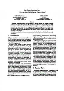
5.5 Performance For the tests illustrated below we used a large model with 296,850 surfels to get reliable results. For each surfel we made a query for its nearest neighbors. We did the same for the model of Fig. 5.7 which contains 56,194 surfels, of which 3748 surfels are query surfels (red) and the rest are the data points of the k-d tree. The results were very similar. All measurements are done with a 1.8 GHz Pentium IV with 1 GB RAM. The comparison is illustrated in the Figs. 5.8 and 5.9 where we used a bucket size of 1 point and in the Figs. 5.10 and 5.11 with a bucket size of 10 points per bucket. It is easy to see that our algorithm is considerably faster than ANN in all cases. For example, for the nearest neighbor of all query points with a bucket size of 10 our algorithm needs only half the time of ANN. Especially interesting is that with larger neighborhood size the performance of ANN decreases exponentially while the computation time of our algorithm is about linear to the neighborhood size. The reason is probably that ANN uses a linear list instead of a priority queue (a binomial heap) for keeping the (sorted) nearest neighbors. However, generally only the query time for few neighbors is important. Although not so important as the query performance we also compared the time needed for building the k-d tree. The results are shown in Table 5.1. Again our algorithm is much faster than ANN. A reason is that we do not have to map (and therefore to copy) our data to the data structures of ANN. Of course the building gets faster with larger bucket size. Table 5.1:

k-d tree build time for 296,850 surfels. new k-d tree

ANN

bucket size = 1

771 ms

1329 ms

bucket size = 10

406 ms

953 ms

We also compared the two algorithms in practice. For that we used the collision detection test described in Section 10.2.1 and applied the robust collision detection algorithm (see Section 6.3) where we used a k-d tree with a bucket size of 10 points per bucket for the nearest neighbor queries. The figures can be interpreted as follows: until time step 20, the nearest neighbor query does not play a substantial role because we have only a few deformable surfels which are close to the zero region and therefore checked for collision. Time variations are due to measuring inaccuracy. When the number of queries gets higher we can observe that the difference between our algorithm and that of ANN gets larger. Again, our algorithm is always faster than ANN, sometimes substantial. Further, we compared the performance of our algorithm for different bucket sizes and different neighborhood sizes. As can be seen in the Figs. 5.12 and 5.13, the bucket sizes have a great impact on the performance. However, we are not aware of that this has been discussed in the literature yet. The difference in speed is especially large when we compare small bucket sizes. For our test with a bucket size of 10 we are always faster than with a smaller bucket size. For larger bucket sizes as e.g. 20 the algorithm is slower for only a few neighbors, but gets faster for many neighbors as expected. We made the same test for several models of different sizes (number of surfels), e.g. for the dinosaur model shown in Fig. 5.7. We found that using a bucket size of about 10 data points results in a great improvement on performance compared with a bucket size of 1, independent of the number of neighbors. This proved to be true also for the ANN k-d tree. Therefore we suggest using a bucket size of about 10 for all queries except if the neighborhood size is very large. Then a larger bucket size may be advantageous.

5.5 PERFORMANCE

25

60000

50000

time (ms)

40000

new k-d tree

30000

ANN

20000

10000

0 0

10 20 30 40 50 60 70 80 90 100 110 120 130 140 150 neighbors

Comparison of our algorithm with ANN for 1 to 150 neighbors with a bucket size 1.

Figure 5.8:

14000

12000

time (ms)

10000

8000 new k-d tree ANN 6000

4000

2000

0 0

5

10

15

20

25

30

neighbors

Figure 5.9:

Comparison of our algorithm with ANN for 1 to 30 neighbors with a bucket size 1.

26

5. K-D TREE

45000 40000 35000

time (ms)

30000 25000

new k-d tree ANN

20000 15000 10000 5000 0 0

10 20 30 40 50 60 70 80 90 100 110 120 130 140 150 neighbors

Comparison of our algorithm with ANN for 1 to 150 neighbors with a bucket size 10.

Figure 5.10:

10000 9000 8000

time (ms)

7000 6000 new k-d tree

5000

ANN

4000 3000 2000 1000 0 0

5

10

15

20

25

30

neighbors

Figure 5.11:

Comparison of our algorithm with ANN for 1 to 30 neighbors with a bucket size 10.

5.5 PERFORMANCE

27

25000

time (ms)

20000

bs 1 bs 2 bs 3 bs 4 bs 6 bs 8 bs 10 bs 15 bs 18

15000

10000

5000

0 0

10

20

30

40

50

60

70

80

90

neighbors Figure 5.12:

Comparison of the performance with different bucket sizes (bs) and different neighborhood sizes from 1 and 100.

4000 3500 bs 1

time (ms)

3000

bs 2 bs 3

2500

bs 4

2000

bs 6 bs 8

1500

bs 10 bs 15

1000

bs 18

500 0 0

5

10

neighbors Figure 5.13:

Comparison of the performance with different bucket sizes (bs) and different neighborhood sizes from 0 to 10.

28

5. K-D TREE

collision detected

350

collision detection time (ms)

300

250

200

150

100

50

0 1

11

21 steps CD with newtime k-d tree

Figure 5.14:

31

41

CD with ANN

Comparison of our algorithm with ANN using the robust collision detection algorithm.

5.6 Summary & Discussion In this section, we summarize and discuss the achieved results with respect to our goals. The performance of our algorithm is considerably better than that of ANN as shown in the last section. The performance gain changes with different models, however, we have not found a case yet where our algorithm was slower than ANN. This is also true for the building time of the k-d tree. The algorithm and classes are kept small and clear, implemented with only a few lines of code. The interface to the algorithm is very simple and easy to comprehend. It uses the data structures of Pointshop3D and therefore no conversions or wrappers are needed. We achieved a considerable saving of memory. Therefore, our algorithm is capable of handling very large models with millions of surfels. Range queries are an additional feature which can be used for searching the nearest neighbor within a certain distance. This feature has been implemented with little additional effort and we make already extensive use of it, as e.g. for the particle simulation (see Chapter 12). Finally we have tested our algorithm thoroughly and compared it with ANN. For this purpose we developed a test application which allows test queries on models in a natural way using the selection tool. When testing the performance of our algorithm we found that it can be improved by using a bucket size of about 10 data points, yielding good results for all neighborhood sizes.

6 6Collision Detection Algorithms

In this chapter we use the definitions of Chapter 4 to present a simple intersection detection algorithm for our application. We extend this algorithm to make use of temporal coherence. We improve the algorithm further such that we finally get a very robust and efficient collision detection algorithm.

6.1 A Simple Algorithm In our application a part of the model is deformable and the rest (the zero region) is rigid as described in Section 3.3. Using the Def. 4.1 and 4.2 we can now easily write an algorithm for detecting collisions between the rigid and the deformable surfels, see Code 6.1. For finding the nearest neighbor we use a k-d tree (see Chapter 5) as a spatial data structure, which we compute in a preprocessing step. SurfelList detectCollision(DeformableSurfels m1, ZeroSurfels m2) { SurfelList surfelList = empty; foreach s1 in m1{ find_nearest_neighbor(s2 in m2, s1.position); d = s1.position - s2.position; if (scalarProduct(d, s2.normal) < 0) { surfelList.add(s1); } } return surfelList; }

Code 6.1:

A simple algorithm returning the deformable surfels which intersect with the zero region.

6.1.1 Problems and Heuristic Solutions First note that our application does not fulfill the conditions of our collision definition because the zero surfels alone (separated from the deformable surfels) do not represent a closed volume. Fig. 6.2 illustrates in 2D a model which causes problems. The deformable part of the model is 29

30

6. COLLISION DETECTION ALGORITHMS

Figure 6.2:

Problems with not closed zero region.

shown in green, the zero region is shown in black. s 2 is the nearest surfel to the deformable surfel s 1 . Because s 2 is on the boundary between the zero and the deformable region we call it a boundary surfel. As can be seen in Fig. 6.2, the angle between d and n 2 is between S e 2 and 3 ˜ S e 2 , and therefore d x n 2  0 , although there is no collision. The problem is that the algorithm uses the tangential plane (shown as dashed black line) of the boundary surfel as “elongation” of the model. All deformable surfels which have s 2 as nearest surfel and are between these two planes are considered as being inside the model. We can improve this if we define that deformable surfels which have a boundary surfel as nearest neighbor do not intersect the model. Because it is very unlikely that a collision occurs at the boundary this restriction works well in practice. For this solution we have to mark all boundary surfels. The boundary surfels can be found by determining the one ring (the surrounding neighbors) of each deformable surfel. The zero surfels of the one ring are boundary surfels. Because we do not have any connectivity information we approximate the one ring as follows: we search for a number n of nearest neighbors of a surfel and then determine which of these surfels are zero surfels. The i (i < n) nearest zero surfels are marked as boundary surfels. With larger n the chance for getting all surfels of the one ring increases but it is less efficient. The choice of i depends on if it is more important to get all zero surfels of the one ring or if preferably no zero surfels should be taken which do not belong to the one ring. Because we assume that there is no collision in the direct region of the boundary surfels and we want to make sure that no false collision detection occurs we choose a larger i. In our current implementation, we use n = 10 nearest neighbors and i = 5 nearest zero surfels.

Figure 6.3:

Two examples of surfel pairs of a non-convex surface.

Problems may also be caused by non-convex models. An example is shown in Fig. 6.3. Again, for both s 1 and s 1 c the angle is between S e 2 and 3 ˜ S e 2 although no collision occurs. In the case of s 1 we can use the same heuristics described above because s 2 is again a boundary surfel.

6.1 A SIMPLE ALGORITHM

31

However, this is not possible for s 2 c . One solution would be to use a (tight fitting) bounding volume which encloses the zero region. Then we can test if s 1 c is inside the bounding volume, otherwise there is surely no collision. We present bounding volumes in the following chapters. If we have no bounding volume we might assume that the deformation is only small per step. Then only surfels which are “close enough” to their nearest surfel are candidates for belonging to a collision, respectively not belonging to a collision anymore. Definition 6.1: A deformable surfel s 1 with nearest surfel s 2 can only change its collision state if s 2 is not a boundary surfel and d  t + r1 + r2 ,

(6.1)

where t is the length of the translation of the deformable surfels in this step and r 1 r 2 is the radius of the surfels s 1 and s 2 respectively. With “change of the collision state” we mean that we know for each surfel if it intersected the surface in the last step (assuming that we know the collision state at the beginning). If the surfel does not satisfy the definition given above we simply keep its state. Because using the norm of a vector means that we have to compute the square root, which is a quite expensive operation, we approximate Eq. 6.1 with 2

2

2

d  t +  r1 + r2 .

(6.2)

Remember that we assume that the transformation is only small. This assumption is necessary anyway because we make only static tests, see Section 3.3. Although the heuristics might prevent us from having a wrong collision detection for concave regions, we cannot detect collisions which arise from concave deformations. We call such collisions concave collisions, an example is shown in Fig. 6.4 . Further we have to estimate the translation vector if we have other transformations than pure translations, e.g. for rotations. In Section 6.3 we present a more robust solution which does not require the transformation vector and is also able to detect concave collisions.

Figure 6.4:

Example of a concave collision. The colliding part is shown in red.

6.1.2 Spatial Coherence A query for the closest neighbor is quite expensive (see Chapter 5). Therefore we should reduce the number of queries if possible. For that, we can use the considerations made to proof Lemma 4.1 in Section 4.2. There we used that all points in a sphere with center at the deformable surfel position s and radius d have the same inside/outside state as s. Remember that if we have a discrete model this is only correct if the model was sampled densely enough. If we know the

32

6. COLLISION DETECTION ALGORITHMS

collision state of a surfel s, all deformable surfels s which lie in the sphere with center s and radius d have the same collision state as s. This means that we have to find all deformable surfels s which fulfill 2 2 d !  s – s .

(6.3)

For that, we could use a range query on a spatial data structure. Because the position of the deformable surfels change with every deformation, we would need a data structure which can be efficiently updated. We could use the query grid which we apply to our particle system (see Section 12.3.3), however, this is still too expensive. In practice we use a list of deformable surfels. Suppose we have n deformable surfels and we have tested the i-1 first surfels. For the i-th surfel, we compute the distance d and then check the n-i-1 last surfels if they fulfill Eq. 6.3. If we find such a surfel we remove it from the list and add it directly behind the i-th surfel. Suppose we have found k surfels. We then continue with the i+k+1-th surfel for testing it for intersection. However, testing all remaining surfels makes only sense if the probability is large that at least a certain number of surfels satisfies Eq. 6.3. The probability gets larger with larger radius d of the sphere. So we should test for this condition only if d 2 ! H 2 . A good choice for H would be to make it proportional to the average sampling density of the deformable region. However, if we cannot assure a constant average sampling density we would have to recompute it after each deformation step. This is clearly to expensive, so we tried other approaches. We made good experiences using the average distance of d for all tested surfels as H . The simplified pseudo-code of the improved algorithm is given in Code 6.5.

6.2 An Efficient Algorithm Using Temporal Coherence In the last section we already made use of the fact that all surfels inside the sphere with the surfel position s as center and radius d have the same collision state as s. We can further improve this by using temporal coherence to our advantage. In our case temporal coherence means that a surfel moves only slightly during a time step. We refer to Section 2.1 for a definition of temporal coherence. If a deformable surfel is not very close to the nearest surfel of the zero region, i.e. d is large, and if the surfel moves only slightly we have a good chance that the surfel moves such that it stays in the sphere with the original position of s as center and radius d . But as stated above, as long as it is in its own sphere it cannot change its collision state and therefore the intersection test reduces to a test if the surfel is inside its sphere. If the test fails then we have to compute the nearest zero surfel anyway and we can update the sphere with its new center and radius. Of course if the “in sphere” test fails then the test and the update of the sphere need additional computation time. Especially if d is small compared with the transformation vector this might often be the case. There are two cases when d is small: if the surfel is near a boundary surfel or if a surfel is near a collision. In the first case not only d is small but also the deformation scale factor (see Section 3.2). This means that the movement of the surfel is also very small and therefore the chance for being inside the sphere is high. In the second case, the probability of a collision is high and therefore the additional computation time is justifiable. However, as shown in Section 6.4, this new algorithm is superior to the algorithm presented in the last section for all models and situations we have tested so far.

6.3 A ROBUST ALGORITHM

33

SurfelList detectCollision(DeformableSurfels m1, ZeroSurfels m2) { SurfelList surfelList = empty; foreach s1 in m1{ find_nearest_neighbor(s2 in m2, s1.position); if (!s2.isBoundary) d = s1.position - s2.position; if (d.sqrLen() > translation.sqrLen()+(s1.radius+s2.radius)2) { if (scalarProduct(d, s2.normal) < 0) { s1.intersects = true; surfelList.add(s1); } else s1.intersects = false; } else if (d.sqrLen() > H ) { foreach s in notTested(m1) { if (d.sqrLen() > (s1.position-s.position).sqrLen()) { s.intersects = s1.intersects; // collision state of s1 if (s.intersects) { surfelList.add(s); } } } } } } H = average(d.sqrLen()); // average over all computed d return surfelList }

Code 6.5:

Improved pseudo-code of the simple algorithm.

For each deformable surfel we store the center c and the square of the radius r of the sphere. The sphere is initialized in a preprocessing step where we use the position of the surfel as center c and the radius r is the distance to the nearest zero surfel. We can also use the sphere to compute an approximation for the minimal distance to the zero region, respectively the penetration depth G if we have a collision, as follows: G = r– p–c

(6.4)

where p is the actual position of the surfel. This distance can be used for the collision response, see Chapter 11. If we do not use a sphere we have to store the position of the closest surfel for each deformable surfel to get the penetration depth.

6.3 A Robust Algorithm The algorithm presented in this section tries to overcome the problems and shortcomings of the algorithms described in Section 6.1. It avoids the problems originating from the non-closed zero region. Further it is able to detect concave collisions (see Section 6.1.1). The idea of the algorithm is very simple: we classify the deformable surfels as inside the original (= not deformed) model or outside. A necessary condition for a collision is that a surfel changes its state from inside to outside or vice versa. However, this is not sufficient because the deformed region might cross the original deformable region. Therefore we only consider a

34

6. COLLISION DETECTION ALGORITHMS

(a) initial state

(b) collision detected

(c) no collision

(d) (concave) collision detected

Figure 6.6:

Collision detection with an inside/outside classification.

deformable surfel for a collision if its closest surfel from the original model is not an original deformable surfel. Because we use the original model, which we suppose to be closed, for the inside/outside test we avoid the case shown in Fig. 6.2. Fig. 6.6 illustrates some examples in 2D. In (a) the initial state of our model is given. The original deformable surfels are blue, the deformed surfels are green and the zero region surfels are black. We classify a deformable surfel which is inside the original model as inside, otherwise as outside. In the initial state the deformable surfels are classified as outside. Look at the deformable surfel d and assume we move d to its new position dc . Let sc be the closest original surfel to dc . In (b) a normal (convex) collision is shown. Thereby the surfel d changes its state from outside to inside. The nearest surfel sc is not an original deformable surfel, therefore we have a collision. In (c) d is inside the original model and then changes to outside. Because sc is a deformable surfel, this is not a collision. In the last example, d is again inside the model and changes to dc which is outside. This time, sc is not an original deformable surfel and therefore we have a (concave) collision. Of course this might go wrong as shown in Fig. 6.7 (a). If the closest surfel is not a deformable surfel although the deformable region was crossed or vice versa, then a wrong collision state change occurs. This means that a collision might be detected even if there is none or vice versa. Therefore we have to assume again that the deformation is only small per time step. We could reduce the possibility for an error by looking not for the closest surfel but for the surfel which is nearest the break-through point of the straight line ddc . This is an expensive task and could be approximated e.g. by looking for the nearest point ss to ds =  d + dc e 2 (see Fig. 6.7 (b)). The disadvantage is that if ss is not a deformable surfel, we have also to search for sc and therefore the computation costs duplicate. However, it is easy to find a situation where this fails too. Anyway, in practice the algorithm which only looks for sc is very robust and the case described above has never happened in our experiments.

6.4 PERFORMANCE

35

(a) wrong collision detection (b) heuristics Figure 6.7: A wrong collision detection and a possible improvement using heuristics. 6.3.1 Using Temporal Coherence We can further improve the algorithm by using temporal coherence as described in Section 6.2. Because we are now looking not for the closest zero surfel but for the closest surfel of the original model, the nearest surfel will initially be the surfel itself. This means that the sphere is initialized with a radius 0 and afterwards its radius will grow only slowly. We can improve this by “merging” the algorithm described in the last section with the temporal coherence algorithm of Section 6.2. The idea is to initialize the sphere with the distance to the zero region instead to the whole model. Only if the sphere needs to be updated we do this with the original region. With this simple trick we achieved a similar performance as with the temporal coherence algorithm of Section 6.2. The disadvantage is that with this initialization the algorithm might fail to detect collisions when we allow concave deformations. The problem is that the algorithm might not detect the transition over the original deformation region and therefore does not change the inside/outside state. A simple solution is to memorize the position of the last deformation step. If the surfel is not in its sphere anymore and therefore we have to check for a collision, we first compute if the surfel was inside or outside the original model at the last time step. This means that we do an update for the inside/outside state for the last time step. Afterwards we can continue as normal. Of course this additional computation doubles the computation time, but because we have to do it at most once per surfel (remember that we update the sphere with the original region afterwards) this has only a slight influence on the performance as can be seen in the next section. This improvement leads to a significant performance gain. Therefore, for the following discussion we will always use this version of temporal coherence. The pseudo-code for the algorithm is given below.

6.4 Performance We call the simple algorithm of Section 6.1 Simple Algo, the improved version of the Simple Algo Improved Simple Algo (see Section 6.1.2), the algorithm using temporal coherence described in Section 6.2 Temp. Coherence Algo and the most robust algorithm of the previous section which uses temporal coherence as well is called Robust Algo. A discussion of our performance tests is given in Section 10.2.1. A performance comparison of all four algorithms using the test example of Section 10.2.1 is shown in Fig. 6.9. The number of colliding surfels is illustrated in Fig. 10.3. In our performance comparisons the Simple Algo is clearly the looser, while the Improved Simple Algo is already much faster than the Simple Algo but nevertheless much slower than the Temp. Coherence Algo and the Robust Algo. The Robust Algo is only slightly slower than the Temp. Coherence Algo as can be seen in Fig. 6.10.

36

6. COLLISION DETECTION ALGORITHMS

SurfelList detectCollision(DeformableSurfels m1, AllSurfels m2) { SurfelList surfelList = empty; foreach s1 in m1{ if (!s1.isInSphere()) { if (s1.firstUpdate) { s1.firstUpdate = false; find_nearest_neighbor(s2 in m2, s1.oldPosition); d = s1.oldPosition - s2.position; s1.isInside = scalarProduct(d, s2.normal) < 0; } find_nearest_neighbor(s2 in m2, s1.position); d = s1.position - s2.position; s1.updateSphere(d.sqrLen()); bool isInside = scalarProduct(d, s2.normal) < 0; if (s2.isZeroSurfel && (s1.isInside != isInside)) { s1.isIntersecting = !s1.isIntersecting; } s1.isInside = isInside; } if (s1.isIntersecting) { surfelList.add(s1); } else { s1.oldPosition = s1.position; } } }

Code 6.8:

A robust collision detection algorithm using enhanced temporal coherence.

We now try to analyze the performance curves of the different algorithms in detail. We would expect the Simple Algo to have a constant performance because it neither depends on the previous step (temporal coherence) nor on the distance to the zero region. We believe that the reason for the performance increase at the beginning is caching. After 30 time steps, the performance is about constant as expected. The performance of the Improved Simple Algo increases at first because the list gets ordered more and more with every time step. After a collision has occurred, the time for collision detection increases as expected. The increase gets much larger when many deformable surfels are near the zero region because the average distance d decreases (see Section 6.1.2) and therefore too many tests are performed. We believe that this could be improved by using better heuristics. The performance curves for the Temporal Coherence and the Robust Algo are very similar. The performance decreases when we get closer to the zero region. The improvement by temporal coherence depends in our case very much on the sphere radius. Because the radius is the distance of a deformable surfel to the zero region, the performance curve strongly depends on the number of deformable surfels with small distance to the zero region. The Robust Algo is slower than the Temp. Coherence Algo because the computation cost for updating the sphere for the first time is duplicated (see the last section). Further, the Robust Algo has to search all surfels for the nearest neighbor, not only the zero region.

6.4 PERFORMANCE

37

collision detected

2500

time (ms)

2000

1500

1000

500

0 1

11

21

31

41

time steps Simple Algo

Figure 6.9:

Improved Simple Algo

Temp. Coherence Algo

Robust Algo

Performance comparison of the algorithms described in this chapter. collision detected

300

250

time (ms)

200

150

100

50

0 1

11

21

31

41

time steps Temp. Coherence Algo

Figure 6.10:

Robust Algo

Comparison of the Temp. Coherence Algo with the Robust Algo.

38

6. COLLISION DETECTION ALGORITHMS

6.5 Summary & Discussion The advantage of the Simple Algo is its simplicity and that its performance only depends on the complexity of the zero- and the deformable region. The Improved Simple Algo which reduces the number of queries is clearly faster than the Simple Algo. However, when many deformable surfels are near the zero region its performance decreases very strongly. Much better performance is achieved by exploiting temporal coherence. Still the Temp. Coherence Algo suffers as also the (Improved) Simple Algo from using the translation vector for avoiding wrong collision detection in concave regions and restricting possible collisions to nearest surfels which are not boundary surfels. Further, all these algorithms are not able to detect concave collisions correctly. The Robust Algo uses inside/outside classifications for all deformable surfels with respect to the original model. It gets rid of the translation vector heuristics and does not have to differentiate between convex and concave collisions. Although the algorithm may fail in the case of concave deformations, it is very robust in practice and generally only slightly slower than the Temp. Coherence Algo. When we allow dynamic resampling of the deformed region (see Section 3.2) our collision detection algorithms must support the insertion and removal of deformable surfels. This can be done easily with all algorithms described above because no dependencies between the deformable surfels exists. When we use temporal coherence we just test if the split surfel is inside the sphere of its parent surfel. If it is we can take the same sphere, otherwise we initialize the sphere with a zero radius. The k-d tree for the nearest neighbor queries can be computed in a preprocessing step because either only the zero surfels or the original surfels are used. In both cases the data points do neither change the position nor are new data points inserted or existing ones removed. However, this is not possible if we want also to detect self-intersection of the deformable region, i.e. if we want to test if a deformable surfel intersects the deformable region. The k-d tree would have to be updated each time after a deformation, which is either expensive or yields worse query performance. In the next chapters we present state of the art hierarchical algorithms for collision detection which we adapted to point-sampled models. In Chapter 10 we compare and discuss bounding volume hierarchy algorithms with the algorithms described in this chapter.

7 7Bounding Volume Hierarchies

Bounding volume hierarchies (BVHs) are widely used for collision detection of non-convex objects. We first define our requirements on a BVH. Then we discuss different design choices and show how we implemented an efficient and easily extensible base class using C++ templates.

7.1 Introduction The goal of using BVHs is to speed up the collision detection by decreasing the number of primitives which must be tested. This means that in general collision detection with the use of a BVH has to be faster than testing the primitives. As a reference we use the collision detection algorithms presented in Chapter 6. As already mentioned we require our algorithms to be especially fast when no collisions occur because then our interactive application should be nearly as fast as without collision detection. The second requirement we have is that the results of collision detection should not dependent on using a BVH or not. Further, using a BVH should also be possible if the model has millions of points, i.e. efficient memory utilization is crucial. For deformable models it must be possible to update the hierarchy if it does not bound the primitives entirely anymore. We now summarize the requirements for a BVH, where we distinguish between BVHs for rigid and deformable surfaces: • If no collision occurs the collision detection has to be generally faster than using the collision detection algorithms of Chapter 6. • The memory requirements are such that the use of huge models with millions of surfels is possible. • The results of the collision detection have to be accurate. • Additionally for BVHs for deformable models: an efficient update of the hierarchy should be possible. 39

40

7. BOUNDING VOLUME HIERARCHIES

7.2 Base Class for BVHs In our collision detection framework it should be possible to use any kind of BVH. Therefore we need to define an interface which has to be implemented by all BVH classes. Further, collision detection with box hierarchies is very similar with most kind of boxes. This is especially valid for AABBs and OBBs. The only difference between these two boxes is that AABBs are axes aligned while OBBs can be oriented arbitrarily in space (see Chapter 8). Therefore it is reasonable and corresponds to good software design to implement a base class for such box hierarchies to avoid code duplication and use the advantages of object oriented programming. However, because performance and memory requirements are very important, the use of a base class should not decrease the performance or enlarge the memory usage. 7.2.1 BVH Interface In Code 7.1 we present our very simple and general bounding volume hierarchy interface. The numbers on the left are line numbers. We give a short description for each method: 0 1 2 3 4 5 6 7 8

class BVHInterface { public: virtual bool intersects(const SurfelInterface *surfel) = 0; virtual int intersects(BVHInterface *bvh) = 0; virtual void recreate() = 0; virtual void drawHierarchy(QRgb rgb, bool bOnlyLeaves = true); virtual bool updateHierarchy(); virtual bool hasBeenUpdated()const; };

Code 7.1:

The generic BVH interface.

2 This pure virtual method tests if a surfel (a point primitive) intersects the surface defined by the surfels in the hierarchy and returns true if it does. 3 This pure virtual method tests if the surface defined by the surfels in an arbitrary other BVH intersects the surface of this hierarchy and returns true if it does. 4 This pure virtual method is called if it is necessary for the BVH to completely recreate itself, e.g. because the surfel positions have changed and we wish to have a new tight fitting bounding box hierarchy. 5 This method is called if the hierarchy has to be drawn with the color given in rgb for illustration purposes. If bOnlyLeaves is true, only the volume boundings of the deepest level in the hierarchy should be drawn. The empty implementation of the method is thought to be overwritten. 6 This method is called if the surfel positions changed and the hierarchy has to be adapted to the new positions. The update should be very fast because it may be called frequently. This is in contrast to the recreate method which may take longer but might create better fitting bounding volumes. The method returns true if the update was successful. In this interface it does nothing than to return false. 7 This method is used to check if a recreation is necessary, i.e. if since the creation (or recreation) of the tree an update has been done which yielded a not optimal bounding volume.

7.3 A BOUNDING BOX HIERARCHY BASE CLASS

41

7.3 A Bounding Box Hierarchy Base Class We implemented a base class which might be used for most bounding boxes. Thereby we subdivide the tasks of a bounding box hierarchy (BBH, also called a bounding box tree) in a generic and a specific part. The generic methods are implemented by the base class while the specific methods have to be implemented by the specific box classes. Generally speaking, the task of the BBH is to administrate the data and to tell the box class what to do. How to do it is the task of the box class. 7.3.1 Disadvantages of Virtual Methods To realize the generic BBH we use a generic defined box class which serves as an interface for the BBH. The standard way for using polymorphism in C++ [62] is via derived classes and virtual functions. A specific box class is then derived from this interface box class and implements the (pure) virtual functions. However, the use of virtual functions can impose a significant performance penalty. When using virtual functions it is not clear at compile time which function is called. This yields two drawbacks: • Because the compiler does not know which function will be called, it cannot “inline” the function which would avoid the overhead of the function call. This decreases the performance especially when the function is only small and is called frequently. An example for such a function is the intersection test of our box classes, as will be described later. • Because the system knows only at runtime which function to call and this function may be different for each object implementing the virtual function, it has to store for each object a pointer to the virtual functions. This needs at least 4 additional bytes per object. As we will see later, a typical box needs 28 bytes, so if we would use virtual functions this would increase the size for each box at 14%. 7.3.2 Using C++ Templates A very efficient alternative to virtual functions is to use the #define compiler directive, as was done e.g. by [25]. However, the comparison of the different implementations is only possible by compiling each one separately and then to run the programs side by side. Therefore it is not possible to offer different choices at runtime. Further, code duplication often cannot be avoided what makes it difficult to change a part of the code. Finally, the code often gets unreadable. We decided to use C++ templates [4] instead. Templates are mechanisms for generating functions and classes based on type parameters. They provide a generic way to develop reusable code. With respect to usage, there are two basic types of templates: function templates and class templates. Because templates are interpreted at compile time their use yields no efficiency penalty. Nowadays, templates are supported by almost every compiler. 7.3.3 BBH Interface For completeness, we shortly describe some of the public functions of our BBH template (see Code 7.2): 0

Template with a class parameter name CBox

1

BBTree derives from the BVHInterface

42

7. BOUNDING VOLUME HIERARCHIES

template class BBTree : public BVHInterface { public: BBTree(); virtual ~BBTree(); virtual void init(QVector *surfels, Neighbourhood *surfelSearch, unsigned int maxLevel, unsigned int minNOfSurfels, unsigned int maxNOfSurfels); 6 virtual CBox* getRoot() const; 7 virtual void drawHierarchy(QRgb rgb, bool onlyLeaves = true); 8 virtual void recreate(); 9 virtual SurfelInterface* intersects(SurfelInterface *surfel); 10protected: 11... 12}; 0 1 2 3 4 5

Code 7.2:

Interface of the BBTree class.

Initializes the data and creates the whole tree. surfels is an array of surfels, surfelSearch is a search structure based on a k-d tree for looking at the nearest neighbor of a surfel, maxLevel defines the maximum number of levels (height) of the tree, minNOfSurfels the minimum and maxNOfSurfels the maximum number of surfels in a leaf box. As soon as these three conditions are fulfilled the creation process for the current box is stopped. 6 Returns the root box of the tree. 7-9 Overriding the functions of the BVHInterface, see the description in Section 7.2.1.

5

7.3.4 Box Interface Because we use templates we cannot define a generic C++ box interface. Instead each class which has functions with the signature described in Code 7.3 can be used (CBox must be replaced with the name of the box). 0 CBox(); 1 void init(SurfelInterface **surfels, int nOfSurfels); 2)int split(); 3 void draw(QRgb rgb) const; 4 inline bool contains(const SurfelInterface *surfel) const; 5 inline bool isLeaf() const; 6 inline void setChildren(CBox *children); 7 inline CBox* getChildren() const;

Code 7.3:

Signature of the functions of a box class.

0 Constructor 1 Initializes the box such that it contains all surfels. This means that the center of the box and the extent of its axes are computed. 2 Sorts the surfels and returns the index value of the surfel array at which the box is split. 3 Draws the box with the rgb color. 4 Returns true if the surfel is inside the box. 5 Returns true if the box is a leaf.

7.3 A BOUNDING BOX HIERARCHY BASE CLASS

43

6 Sets an array of child boxes. 7 Gets the child boxes. Note that although we were always talking of boxes we have implemented a sphere tree the same way (see Chapter 9). 7.3.5 Example Box Structure Vector3D Vector3D CBox

m_center; m_extent; *m_children;

Code 7.4:

Example of a box structure.

An example box structure is shown in Code 7.4. A Vector3D is an array of 3 floats. Therefore this structure needs 28 bytes. Note that we have only one child pointer to an array of children. This allows in principle as many children as needed. Further it saves us one pointer and we can profit from caching if we use both children one after the other. A pointer to the second child can be simply received by increasing the children pointer at one, i.e. getChildren() + 1 returns a pointer to the second child. As you might have noted a box may not need to contain any information of which and how many surfels it contains. This is also true if the box is a leaf. The reason is that we generally do not use the data of a leaf but use a global query to check for intersection in the narrow phase (see Section 7.3.7). However, if the data are needed we can store a pointer to the start position in the surfel array together with the number of the surfels in this box. This needs 8 additional bytes. We could save these 8 bytes for half of the boxes if we store the number of surfels and the pointer to the surfels only in the leaves. Remember that we do not want to use an abstract class (class with virtual functions) for the box classes. Otherwise the children pointer could point to this generic box class and we would not mind if this class is a node or a leaf. However, we could use the children pointer anyway by pointer casting. But then we still have the problem of identifying if the pointer points to a node or a leaf class. We could use dynamic type checking at runtime but this is much too expensive. If we assume that all classes are two bit aligned (which should be the case anyway for efficiency reasons), we could use the least significant bit of each child pointer to decide if the child is a box or a leaf. However, there is always the trade-off between memory and performance efficiency. Because these operations are executed very often, we lost about 10 - 20% of performance. Anyway, if we store this additional information of the surfels in each node we can use it to our advantage in several cases. For example we are able to stop at any level of the hierarchy, i.e. we can build a tree with more levels and then only use some of the levels without rebuilding the tree. This is often used for time-critical applications which stop after some time and then use the information gained until then. 7.3.6 Building the Tree A tree can be created in many ways. First we have to decide if we want to build the tree topdown, bottom-up or with incremental insertions. Top-down approaches are the most commonly used in practice because they can be naturally implemented with recursive “fit-and-split” operations. A top-down method starts with a box that encloses all surfels.

44

7. BOUNDING VOLUME HIERARCHIES

In contrary a bottom-up approach starts by using boxes for each surfel and then merges the boxes until there is only one box left. Incremental insertion adds surfels to the BVH one at a time until all surfels have been incorporated into the tree. The insertion can be done by either traversing the tree down to the leaf and enlarging the BVs when necessary or by merging it to some nearby leaf node and then updating the parent boxes. For our generic tree construction algorithm we use a top-down approach because it allows us to stop when the tree has reached a specified height, avoiding that the whole tree has to be created. Generally, a tree can have an arbitrary number of children (called the degree of the tree). In practice, binary, 4-ary and 8-ary trees are used. We use binary trees because of two advantages: firstly, they are simpler and faster to compute since there are fewer options in how one splits a set in two than how one partitions a set into several subsets. Secondly, analytical evidence suggests that binary trees are better than trees with a higher degree. For a discussion we refer to [34]. A disadvantage is that with lower degree we need generally more nodes and therefore more memory. The most difficult decision is how to split a box. Because this is a specific process for each kind of a box, the box class must implement this. Our recursive implementation of the tree creation method is given in Code 7.5. template void BBTree::createTree(CBox *root, SurfelInterface **surfels, unsigned int nOfSurfels, unsigned int level) { if (level == 0 || nOfSurfels split()+1; CBox *children = new CBox[2]; children[0].init(surfels, cut); children[1].init(surfels+cut, nOfSurfels-cut); createTree(children, surfels, cut, level-1); createTree(children+1, surfels+cut, nOfSurfels-cut, level-1); }

Code 7.5:

Recursive creation of the tree.

7.3.7 Intersection Test We can either test a single surfel for intersection with a BVH or test two BVHs for overlapping. For the intersection test with a surfel we distinguish between a broad and a narrow phase. In the broad phase the boxes are tested whether they are intersected by the surfel. To avoid the overhead of recursive functions we use a First In First Out (FIFO) queue to traverse the tree. With a FIFO queue we do a breath-first search which can also be advantageous if we want to stop after some time and then use the information we have (see also Section 7.3.5). If we are at a leaf we perform the narrow intersection test to exactly detect if the surfel collides with the surface which is represented by the surfels of the BVH. Remember that for an exact intersection test of a surfel s we need to find the closest surfel to s. Unfortunately we cannot do this by simply looking for all surfels in the intersecting box because the nearest surfel may be in another neighbored box. There are several possibilities for finding the nearest surfel. The most simple approach is to use a “global” query similar as we did

7.4 SUMMARY

45

template bool BBTree::intersects(const SurfelInterface *surfel) { CBox *box; m_fifoQueue->reset(); m_fifoQueue->enqueue(m_root); while (!m_fifoQueue->isEmpty()) { box = m_fifoQueue->front(); m_fifoQueue->dequeue(); if (box->contains(surfel->getPosition())) { if (box->isLeaf()) return narrowIntersection(surfel); else { m_fifoQueue->enqueue(box->getChildren()); m_fifoQueue->enqueue(box->getChildren()+1); } } } return false; }

Code 7.6:

Surfel intersection test using a FIFO queue.

for the collision detection methods described in Chapter 6. As a spatial data structure we use a k-d tree. Otherwise, we could make a query directly in the AABB hierarchy starting with the intersecting box. However, this is more complicated than with a k-d tree and therefore we believe that this approach would be slower. Further we would need to store additional information in each box to achieve efficient queries. Therefore we use a global query with a k-d tree in our current implementation. However, note that the narrow intersection test could be overwritten by any derived class of BBTree. Because the box interface is very generic it is difficult to write a generic intersection test function for two bounding volume hierarchies. Generally it is necessary to check at run time which kind of BVH (i.e. which derived class) is used and then to provide an intersection test in dependence of this class. However, for the narrow phase the generic narrow intersection function can still be used.

7.4 Summary In this chapter we introduced a generic bounding volume hierarchy interface. Each BVH class which implements this interface can be used in our collision detection framework. Further we implemented a base class for box and sphere BVs which does all the generic work and delegates the specific tasks to the BV. Because we use templates the base class is created at compile time, and therefore we have no performance loss.

46

7. BOUNDING VOLUME HIERARCHIES

8 8AABB & OBB Trees

Axis-aligned bounding boxes (AABBs) and oriented bounding boxes (OBBs) are two of the most popular bounding volume hierarchies. We chose AABBs because of their fast intersection tests and efficient update feasibility and OBBs because of their tight fitting. In the next sections we show how we build the AABB and OBB tree and how to perform intersection tests. Further we propose an adapted hybrid updating of AABB trees which is generally faster than all other known update methods. Finally, we compare AABB with OBB trees.

8.1 AABB Tree In this section we present a hierarchical model representation using axis-aligned bounding boxes (AABBs). Because we test only for self-intersection in our application, the coordinate system for all AABBs is the same. This is useful for fast intersection tests as explained below. First we show how to efficiently create a hierarchy which is nevertheless tight fitting for fast intersection rejection. 8.1.1 Building the AABB Tree A box hierarchy originates from splitting the bounding boxes. Often the partitioning plane is chosen along the longest axis. There are different choices of how to split this axis, e.g.: a using the median of the AABB, thus splitting the box in two equal halves, b subdividing the set of surfels in two sets of equal size which yields an optimal balanced tree or c building a half balanced tree, i.e. the larger subset is at most twice as large as the smaller one which minimizes the overlap of the subsets’ AABBs projected onto the longest axis. As van den Bergen [68] found out, the best performance is achieved with (a). Other approaches use the splitting rule which yields “the best children”. For each possible split the child boxes are computed and then the best split is chosen. Examples for this kind of splitting rules are the Min Sum, where the axis is chosen that minimizes the sum of the volumes of the two resulting children, and the Min Max, where the axis is chosen that minimizes the larger of the volumes of the two resulting children. Although these methods tend to yield better fitting bounding volumes than the others, they use considerably more preprocessing time. 47

48

8. AABB & OBB TREES

We choose the axis to which the splitting plane is orthogonal to as the axis at which the projected points have the biggest spread (this rule is called Splatter by Klosowski et al [34]). We partition this axis using the mean of the projected points. Computing the mean needs time O  n . Afterwards we separate the array into elements smaller and larger than the mean. This needs also time O  n , therefore the splitting has a linear time complexity O  n . Another possibility for choosing the split point is to use the median instead of the mean, which has also a linear time complexity. The median has the advantage that it yields optimal balanced trees. However, Klosowski [34] showed that in all his experiments the mean always produced a hierarchy with smaller total volume than when using the median, and therefore the performance was always better when using the mean. In Fig. 8.2 we show the AABBs at different levels in the hierarchy. Note that we are lucky in this example because the plane is aligned with the coordinate axes and therefore the AABBs suits it very well. However, as you can see, AABBs have problems to fit curved regions tightly. 8.1.1.1 Time Complexity for Building the AABB Tree In the worst case, the box is split such that always only one surfel is on one side. If you look at Code 7.5 in Section 7.3.6, the time for creating such a hierarchy is Tn = Sn + T1 + Tn – 1 ,

(8.1)

where S(n) is the time needed to split the box (for our implementation this is O  n as shown above) and T(1) needs constant time O(1). This yields 2 ˜  n + 2 - T  n = n + 1 + T  n – 1 = n + 1 + n – 1 + 1 + } + 1 + 1 = n----------------------= On 2

(8.2)

In the best case, the box is always split such that the surfels are subdivided into two sets of equal size. This yields a time complexity of n n T  n = n + 2 ˜ T § ---· = n + 2 ˜ --- + } + 2 = 3 ˜ n – 2 = O  n © 2¹ 2

(8.3)

Note that if the surfels are uniformly distributed this is also the average complexity. 8.1.2 Intersection Tests 8.1.2.1 AABB/Surfel We can test the deformable surfels against a hierarchy of zero surfels for intersection. The generic procedure is described in Section 7.3.7. What is missing yet is the intersection test between the box and the surfel which has to be provided by the box class (see Code 7.6). The AABB with center b center and extent b ext intersects the sphere with center s center and radius r if b centerd – s centerd  b extd + r

(8.4)

for all dimensions d  ^ 1 2 3 ` . 8.1.2.2 AABB/AABB Suppose we test an AABB tree of deformable surfels with an AABB tree of rigid surfels for intersection. We start with the root boxes and test if they overlap. If they do then the children of one of these are tested against the other and so forth until two boxes do not intersect or both

8.1 AABB TREE

Figure 8.1:

Figure 8.2:

49

(a) 1 level

(b) 3 levels

(c) 5 levels

(d) 8 levels

Different levels of the AABB hierarchy for the zero region (blue).

(a) 1 level

(b) 3 levels

(c) 5 levels

(d) 8 levels

Different levels of the OBB hierarchy for the zero region (blue).

50

8. AABB & OBB TREES

boxes are leaves. We tried following heuristics to choose the box whose children have to be tested next: a the box with the largest volume, b the box with the larger diagonal, c similar to (b) but with only summing up the length of the box extents and d the box containing more surfels. We found the efficiency of these methods to be inverse to the number of operations. (b) using 6 multiplications and 6 additions was the slowest, followed by (a) with 6 multiplications and (c) with 3 additions. The best performance had (d) which needs no floating point operations (except one comparison). If a box of a tree is a leaf box, the boxes of the other tree are compared until a leaf is reached or two boxes do not overlap. If both boxes are leaves then we take the surfels of the box containing the deformable surfels and perform the narrow intersection test for each surfel as described in the last chapter in Section 7.3.7. It will often happen that a box intersects with more than one box. Because we use a global query we only have to test the surfels of each box at most once. Therefore we need to remember which leaf box has already been tested. In order to not have to set the state of all leaf boxes back to “not yet tested” we use an integer flag which is increased each time two AABB hierarchies are tested for intersection. We can even use this information for nodes in the hierarchy which are not leaves. If both children were tested then we can set the flag also for the parent node and we do not have to perform any intersection tests with this node again. The whole procedure is shown in Code 8.4.

Figure 8.3:

Intersection test for two boxes using dimension reduction.

Two AABBs can be efficiently tested for intersection by projecting their extents onto the coordinate axis and then testing the intervals for overlap. This is also called dimension reduction. An example with two boxes is shown in Fig. 8.3. Assume we have a box a and a box b then this two boxes overlap if and only if b centerd – a centerd  b extd + a extd

(8.5)

for all dimensions d  ^ 1 2 3 ` . Therefore we need in the worst case (when the two boxes intersect) 6 floating point operations, three absolute value operations and three comparisons.

8.2 OBB TREE

51

int AABBTree::intersects(AABBox *deformBox, AABBox *box) { if (deformBox->flag == flag) { return 0; // already tested for intersection -> return } if (box->intersects(deformBox)) { if (box->isLeaf()) { if (deformBox->isLeaf()) { deformBox->flag = flag;// set box as tested // exact intersection test for all surfels in deformBox return narrowIntersection(deformBox); } int n = intersects(deformBox->getChildren(), box) + intersects(deformBox->getChildren()+1, box); if (deformBox->getChildren()->flag == flag && deformBox->getChildren()[1].flag == flag) { // if both children are tested then set this box also as tested deformBox->flag = flag; } return n; } else if (deformBox->isLeaf()) { return intersects(deformBox, box->getChildren()) + intersects(deformBox, box->getChildren()+1); } else if (deformBox->getNOfSurfels() > box->getNOfSurfels()) { // test with the box with less surfels int n = intersects(deformBox->getChildren(), box) + intersects(deformBox->getChildren()+1, box); if (deformBox->getChildren()->flag == flag && deformBox->getChildren()[1].flag == flag) { deformBox->flag = flag; } return n; } else { return intersects(deformBox, box->getChildren()) + intersects(deformBox, box->getChildren()+1); } } }

Code 8.4:

Intersection test of two AABB trees.

8.2 OBB Tree Oriented bounding boxes (OBBs) can be oriented arbitrarily in space and therefore generally fit the object more tightly than AABBs. However, the intersection test is more expensive. Gottschalk et al. have shown how to efficiently test two OBBs using the separating axis theorem [26]. Their collision system for triangles using OBBs is called RAPID and can be freely downloaded at www.cs.unc.edu/~geom/OBB/OBBT.html. In the next sections we present our implementation of OBBs for point-sampled models.

52

8. AABB & OBB TREES

8.2.1 Building the OBB Tree We first show how to compute a tight fitting OBB for a collection of surfels and then how to construct the tree, where again the BBTree template is used. As already mentioned the three orthogonal axes of the OBB can lie arbitrarily in space. The task consists in finding directions for these axes such that the bounding box fits the objects as tight as possible. For that we use principal component analysis (PCA), i.e. computing the directions of most and least spread of the points using the covariance matrix. If we have the surfel positions p i of a surfel collection with n surfels, the covariance matrix is computed as follows: 1 n–1 i C j k = --- ˜ ¦ p ˜ p ik , i=0 j n

1 d j k d 3

(8.6)

1 n–1 i where n is the number of surfels, p i = p i – P and P is the mean value, i.e. P = --- ˜ ¦ p . i=0 n The covariance matrix is a 3 u 3 symmetric matrix. Two of the three eigenvectors, which are mutually orthogonal, point to the direction of maximal and minimal variance. Thereby the eigenvector with the smallest eigenvalue points to the direction with the least variance, while the eigenvector with the largest eigenvalue points to the direction with the largest variance. The normalized eigenvectors are then used as a basis for the OBB. This approach can fail if there are surfels at the interior of the model. It can be improved by using only the surfels belonging to the convex hull. However, because in our application we assume that the surfels represent the boundary we expect that no surfels are at the interior of the model, and therefore we can avoid the (most) expensive step of creating a convex hull first. The OBB is stored similar to the AABB with the center coordinate, the extent of the axes and the number of surfels. Additionally, we store the three eigenvectors in a rotation matrix. The rotation matrix transforms a point from the canonical coordinate system to the OBB proper coordinate system, spanned by the three eigenvectors. If we want to save memory we could store the rotation matrix into a quaternion [58, 59]. This would need only 4 ˜ 4 bytes instead of 9 ˜ 4 bytes for the matrix, however, the price would be a worse performance. The tree is built using the top-down approach of the BBTree (see Section 7.3.6). We split an OBB along the axis with the largest spread, i.e. the axis corresponding to the eigenvector with the largest eigenvalue. The position of the splitting plane is again taken as the mean of the points projected onto this axis. Creating the OBB tree takes time O  n ˜ log 2 n if the surfels are reasonable balanced and O  n 2 in the worst case. For details we refer to [25]. Different levels of the OBB tree for the zero region of a plane are shown in Fig. 8.2. Note that a quadrate is the worst case for an OBB because it aligns with the diagonal. However, already with 5 levels the circle is fit quite well. With 8 levels, we have an obviously better fitting of the zero region than with the AABB tree. 8.2.2 Intersection Tests 8.2.2.1 OBB/Surfel Testing if an OBB intersects a surfel is very similar to the AABB/surfel test described in Section 8.1.2. In fact it is the same if we transform the surfel into the coordinate system of the OBB. This can be done by rotating the distance vector of the surfel center and the OBB center into the OBB coordinate system and then compare it with the extent of the OBB, i.e.:

8.2 OBB TREE

53

A surfel with position p and radius r intersects a box b with rotation matrix R if and only if  R ˜  b center – p d d b extentd + r

(8.7)

for all dimensions d  ^ 1 2 3 ` . 8.2.2.2 OBB/AABB At the moment, we only offer AABB trees as bounding volume hierarchies for the deformable surfels, see the next section. Therefore, we have to test OBBs only against AABBs. This makes life easier because the rotation matrix of the OBB is also the relative matrix to the AABB. Therefore we can avoid to compute the relative matrix to a frame of reference in a preprocessing step as suggested by Gottschalk [25]. We next describe shortly the overlap test based on the separating axis theorem (SAT). For details we refer to [25]. Definition 8.1: A separating axis is an axis on which the projections of two polytopes do not overlap. Separating Axis Theorem 8.1: Two convex polytopes A and B are disjoint if and only if there exists a separating axis which is orthogonal to a face of either polytope or orthogonal to an edge from each polytope. Because an OBB has only 3 distinct face normals and 3 distinct edge directions it is sufficient to test 15 axes. Further simplifications occur because the set of face normal directions and the set of edge directions are the same, and because these directions are mutually orthogonal.

Figure 8.5:

L is a separating axis for OBBs A and B because A and B become disjoint intervals under projection onto L [25].

Gottschalk et al. further simplified the tests by projecting the center points onto the axes to get the separation between the interval midpoints. This is shown in Fig. 8.5. The width of an interval can also be computed by simply projecting any three mutually orthogonal edges of a box onto the axes and summing the lengths of their images. The intervals are disjoint if and only if T x L ! rA + rB , where r A and r B are the interval lengths, i.e. r A =

¦i a

(8.8) i

i

˜A xL .

54

8. AABB & OBB TREES

The computation is most efficient when choosing L such that L = R Ai , L = R Bi and L = R Ai u R Bj for i j  ^ 1 2 3 ` . Note that in our case R Ai is the identity matrix, which further simplifies the computation. This yields for L = R Ai and L = R Bi respectively following tests:  T A – T B d ! a d + b 1 ˜ R B1d + b 2 ˜ R B2d + b 3 ˜ R B3d and

(8.9)

 T A – T B 1 ˜ R B1d +  T A – T B 2 ˜ R B2d +  T A – T B 3 ˜ R B3d !

(8.10)

a d + b 1 ˜ R B1d + b 2 ˜ R B2d + b 3 ˜ R B3d for d  ^ 1 2 3 ` . As Gottschalk et al. stated this needs in the worst case (when an intersection is found) about 200 operations for the 15 axes tests. However, we follow van den Bergen [68] who uses only the 6 axes tests given in the Equations 8.9 and 8.10. He called this the SAT lite test. However, with SAT lite an overlap may be reported even if there is none. This may yield more overlap tests, but the tests are considerably faster. As van den Bergen found out using this simplified test yields incorrect results in only 6% of the time (note that with incorrect results we mean that an overlap test failed, not an incorrect collision detection result). We compared the two tests and got the same result as van den Bergen, i.e. that the performance benefits from a cheaper but sloppier box overlap test in all cases.

8.3 Updating If we also use a bounding box hierarchy for the deformable surfels we have to update it every time the position of a surfel changes such that the boxes enclose again all their surfels. An update should also be done if new deformable surfels are created or existing ones removed. Generally there are two possibilities for updating: creating a new best fitting bounding box hierarchy or refitting the existing boxes of the hierarchy. While the former generally creates better fitting bounding boxes with fewer overlaps, the latter is usually faster. In fact the building of a hierarchy is often seen as not to be time critical because it is assumed that it is done only once (or rarely), but many intersection tests have to be executed, therefore the tree is optimized for the intersection tests. Updating an OBB hierarchy is much more complex and uses significantly more time than updating an AABB hierarchy. That is why we chose an AABB tree for the deformable surfels. 8.3.1 Updating of AABBs There are three possibilities for updating an AABB tree: top-down, bottom-up or using a hybrid update. For the bottom-up method we propose a new strategy which is very fast.

Figure 8.6:

The smallest AABB of a set of surfels encloses the smallest AABBs of the subsets in a partition of the set.

8.3 UPDATING

55

An AABB tree can be updated efficiently bottom-up because of the following property [68] (see Fig. 8.6): Assume there is a set S 1 and a set S 2 containing each a subset of the surfels in the set S such that S 1 ‰ S 2 = S , and let B 1 and B 2 be the smallest AABBs of S 1 and S 2 respectively. Then the smallest enclosing box B of B 1 and B 2 is also the smallest AABB of S. This yields directly to a bottom-up approach, starting with the leaves. If the box of a leaf has to be readapted then the parent box of the leaf will also be recomputed and so on.

(a) standard bottom-up update

(b) selective bottom-up update

(c) top-down update

(d) hybrid update

Figure 8.7:

Illustration of different update methods. Updating starts at the nodes with red circles, the blue nodes are updated.

Van den Bergen [68] updates all parent boxes until the root is reached (see Fig. 8.7 (a)). We use another approach by only propagating the update if we have to. An update is necessary if the box does not enclose all points anymore, i.e. if it has to be repositioned and/or enlarged (Fig. 8.7 (b)). This is much faster because the propagation can often be stopped early. We can even benefit more if we make the boxes a little bit larger than necessary. The disadvantage is that we might get worse fitting boxes, especially for boxes at the top level. We compensate this with rebuilding the whole tree on idle time, as described in Section 8.3.3. For fast updating we always inform the parent box for which axes a refitting is necessary. We do this by using a bit-code for each axis and bitwise adding the codes to the return value. Then the parent box has to check and recompute the corresponding axes only. In a typical collision traversal, only some of the bounding boxes are needed. A top-down method can profit from that by only updating the nodes which are visited (Fig. 8.7 (c)). These are often fewer nodes than with the bottom-up approach, but the box has to be recomputed each time. Larsson and Akenine-Möller [37] introduced a method called hybrid update which combines efficient bottom-up calculations with selective top-down updates. The goal is to update as few AABBs as possible while still updating the ones in the top of a tree bottom-up. Hybrid updating starts at a specified level instead at the leaves and updates the nodes bottom-up. We use again our modified bottom-up approach for that. All nodes from the root down to the specified level are marked as updated (respectively as being considered for an update). For marking we use again an integer value instead of a boolean. When the tree is traversed and we are at a node

56

8. AABB & OBB TREES

collision detected

350 300

time (ms)

250 200 150 100 50 0 1

11

21

31

41

time steps f = 1.00

Figure 8.8:

f = 0.75

f = 0.50

f = 0.25

f = 0.00

Performance comparison of different update strategies.

which has not been marked yet, the node is tested for update and marked as updated afterwards. So during traversal we use top-down updating. This approach is illustrated in Fig. 8.7 (d). We give the user the possibility to choose between the degree of hybrid updating with a factor f, f  > 0 1 @ . We then update the boxes bottom-up starting at f ˜ # levels . This means that if f = 0 we perform a full top-down updating, while if f = 1 all boxes are updated bottom-up. For all other values, a hybrid updating subject to f is performed. In Fig. 8.8 we compare the collision detection performance with different f values. We used the test method described in Section 10.2.1 with an AABB hierarchy for both the deformable and the zero region. We used a maximum of 10 levels for the zero region and of 15 levels for the deformable region. The hybrid update methods with f = 0.5 and f = 0.75 are generally faster than the bottom-up update ( f = 1 ). This corresponds to the observation made by Larsson and Akenine-Möller [37]. The small performance gain is due to the little time used for updating. With smaller f, we loose more and more performance and the top-down approach ( f = 0 ) is significantly slower than the bottom-up approach. Note that the best value for f depends strongly on the application and on the height of the tree. 8.3.2 Insertion/Removal of Surfels In our collision detection requirements we stated that the algorithm should be able to handle the insertion and removal of deformable surfels (see Section 3.3). This is not a problem as long as we only use BVHs for the zero region. However, if we want also to use a BVH for the deformable region we need to update it every time when new surfels are inserted or existing one deleted.

8.4 CONCAVE COLLISIONS

57

Deletion can be handled efficiently by only marking a surfel as deleted. When we update a box and find a surfel which is marked as deleted we remove it from the box and delete it also physically if it is not in another box anymore. There are several difficulties for inserting new surfels. First we need to find the box where a surfel has to be inserted. It might happen that it cannot be placed in any box, we then have to either create a new box or enlarge an existing box. Further we cannot use an array anymore but need a dynamic structure, e.g. a list. Anyway, if many surfels have to be inserted, what is typically the case during dynamic resampling, the insertion of new surfels in a bounding volume hierarchy is much to slow. We propose two strategies to circumvent the insertion of new surfels: The simplest solution is to ignore the new surfels and take the existing BVH as approximation for the surface. Because in our case a new surfel is created by splitting an old surfel and then applying a relaxation filter, most of the surfels will lie in an existing bounding volume anyway and therefore the approximation will be good. When the BVH is recreated, for example on an idle event (see the next section), the new surfels will naturally be considered for the new hierarchy. Another approach is to test the new surfels separately. This means that we do an intersection test for both hierarchies as normal, and then test the new surfels with the zero hierarchy separately. However, if we have many new surfels this will yield a significant performance loss. An alternative would be to use a spatial data structure, for example a grid, instead. In a grid the insertion could be efficiently done in constant time. We have not tried this, but in the literature object partitions are preferred to space partitions. 8.3.3 Recreation on Idle A drawback of updating is that the boxes in a refitted tree may have a higher degree of overlap than the boxes in a rebuilt tree. Therefore we offer the possibility to automatically rebuilt the tree on an idle event. Rebuilding on idle has the advantage that whenever possible a new best fitting tree is created nearly without delay in the deformation process. However, rebuilding is not always desirable. This is especially the case if the deformation goes forward and back. Then the refitted tree may need fewer updates than a rebuilded tree. That is why we give the user the possibility to only rebuild the tree after the deformation process has finished, i.e. the mouse button is released.

8.4 Concave Collisions The detection of collisions which arise from concave deformations (we call them concave collisions) is also an issue for BVHs. We can use the same solution as described in Section 6.3, i.e. instead of using a BVH only for the zero region we build a BVH for the whole original (not deformed) model. We then classify the deformable surfels according if they are inside or outside the original model. A collision occurs if the inside/outside state changes and the closest surfel is not an original deformable surfel. For details we refer to Section 6.3. However, because surfels which are near the boundary between deformable and zero region generally intersect with at least one BV, this slows down the collision detection significantly. We achieve a more efficient approach by using a similar trick as we applied for using temporal coherence with the Robust Algo (see Section 6.3). We compute the BVH for the zero region as usual, but additionally we store for each deformable surfel its position before the transformation. The inside/outside classification is done with the original model. When a surfel is candi-

58

8. AABB & OBB TREES

date for a collision we compute its inside/outside state before and after the transformation has occurred. If the inside/outside state changes then also the collision state changes, cf. Section 6.3. However, for each surfel which needs to be checked for collision we have to compute the state twice. We can improve this by remembering the inside/outside state together with the “step number”. If the step number is equal to the actual step number - 1 we do not have to compute the state before. This will often be the case because of temporal coherence. The performance of these extended algorithms is compared in the next section, see Fig. 8.12.

8.5 Performance Comparison of AABB/OBB In this section we compare the performance of the AABB tree with the OBB tree. For the illustrated comparisons shown below we used the test example of Section 10.2.1. 8.5.1 Cost Equation For analyzing the performance of the different BVH algorithms, we take the basic cost function introduced by [69] and extended by [36]: T = Nv ˜ Cv + Np ˜ Cp + Nu ˜ Cu

(8.11)

where T : total cost function for collision detection, N v : number of bounding volume pair or bounding volume/primitive overlap tests, C v : cost of testing a pair of bounding volumes for overlap, N p : the number of primitives tested for intersection, C p : cost of testing a primitive for intersection, N u : the number of bounding volumes which have to be updated C u : cost of updating a bounding volume. A bounding volume yields a good performance when • it fits the original model as tightly as possible (to lower N v and N p ), • the overlap test is fast (to lower C v ) and • it can be efficiently updated (to lower C u ). Because we use a global query for testing a primitive for intersection we can assume that C p is constant. 8.5.2 BVH for Zero Region only In Fig. 8.9 we used an AABB respectively an OBB hierarchy for the zero region and tested the deformable surfels with the hierarchy for intersection. As can be seen the use of an OBB hierarchy is clearly faster than the AABB hierarchy. The reason is that for the OBB tree in this example N v is between 30% - 50% lower than that for the AABB tree because of its tighter fitting (see Fig. 8.10), but the cost C v of the test is only slightly higher (maximal 3 addition and 3 multiplication more per test than with an AABB).

8.5 PERFORMANCE COMPARISON OF AABB/OBB

59

collision detected

450 400 350

time (ms)

300 250 200 150 100 50 0 1

11

21

31

41

time steps AABB - Surfels

Figure 8.9:

OBB - Surfels

Performance comparison AABB/OBB tree for the zero region. collision detected

800000 700000

# overlap tests (Nv)

600000 500000 400000 300000 200000 100000 0 1

11

21

31 time steps AABB

Figure 8.10:

OBB

Comparison of N v for AABB and OBB trees.

41

60

8. AABB & OBB TREES

8.5.3 BVH for Zero and Deformable Region We also tested the performance of the OBB and the AABB tree if we use an AABB tree for the deformable surfels. At the beginning, both have about the same performance as can be seen in Fig. 8.11. Then, when we are close to the zero region and for only a few intersections, the OBB tree is faster than the AABB tree. However, for an increasing number of intersections the performance of the OBB decreases strongly. This is also the case for the AABB tree, but the performance drops lower than with the OBB tree. This behavior can be explained as follows: the overlap test cost C v of an OBB tree is about one-order of magnitude slower than that for AABBs [26]. This is because we have to do 6 single tests instead of 3. Furthermore these tests are more expensive. The performance loss is considerable especially if the two boxes overlap because then we have to do all tests. If the two boxes do not overlap the 6 single tests for the OBB can often be aborted already after one or two tests, and therefore the tests are not much more expensive than for the AABB. However, as already discussed N v and also N p is asymptotically lower for an OBB tree. This is why at the beginning, when we have no or only a few intersections, we are faster with an OBB tree and afterwards, when many intersections occur, the AABB tree is faster. collision detected

500 450 400

time (ms)

350 300 250 200 150 100 50 0 1

11

21

31

41

time steps AABB - AABB

Figure 8.11:

OBB - AABB

Performance comparison of the intersection test using an AABB hierarchy for the deformable surfels and an AABB respectively OBB tree for the zero region surfels.

8.5.4 Concave Collisions In Fig. 8.12 we compare the performance of AABB trees which employ the extension for detecting concave collisions with the “normal” AABB trees. As expected the extension yields a significant performance penalty which increases with an increasing number of narrow intersection

8.6 SUMMARY & DISCUSSION

61

collision detected

1200

1000

time (ms)

800

600

400

200

0 1

11

21

31

41

time steps AABB - AABB

Figure 8.12:

Ext. AABB - AABB

AABB - Surfels

Ext. AABB - Surfels

Performance comparison of AABB trees which can/cannot detect concave collisions.

tests. This is also the reason why the performance loss is larger when we use bounding volumes for both regions.

8.6 Summary & Discussion We now summarize the results of this chapter and discuss the advantages and drawbacks of the different approaches. Axis-aligned bounding boxes are built efficiently by choosing the splitting plane orthogonal to the axis with the largest variance at the mean. Objects are often not bounded very tightly because the axes are fixed, but that is also why the intersection test can be performed very efficiently by using dimension reduction. AABBs are suitable for fast updating, where the hybrid method using the modified bottom-up approach showed to be superior to the pure bottom-up or top-down methods. This is especially the case for high trees. Oriented-bounding boxes are computed by choosing the axes along the direction with the largest and smallest variance. Therefore building the hierarchy needs more time than for the AABB tree (see Section 10.2.3 for a comparison of the preprocessing time of different algorithms). They often fit the objects more tightly than AABBs but the intersection test is more expensive, especially for testing an OBB with an AABB for overlapping. Because for an OBB we have to store the rotation matrix we need 36 bytes more per box than for an AABB. This doubles the memory requirements for an OBB. Updating of OBBs is in our case too expensive, however, if the whole object would be transformed (e.g. rotated) we could simply update the rotation matrices. In this case, updating of the OBB tree would be preferable to the AABB tree.

62

8. AABB & OBB TREES

collision detected

600

500

time (ms)

400

300

200

100

0 1

11

21

31

41

time steps AABB - Surfels

Figure 8.13:

OBB - Surfels

AABB - AABB

OBB - AABB

Performance comparison of all BVH approaches.

In Fig. 8.13 we compare the performance (without the extension for concave collisions) for all approaches. For no or few intersections, using an AABB tree for the deformable surfels yields better performance than the direct test of each deformable surfel with the zero region hierarchy. For many intersections, an AABB tree for both regions is preferable to an OBB tree for the zero region and an AABB tree for the deformable region. When we use a hierarchy only for the zero region an OBB tree is generally faster than an AABB tree. When we use the extension described in Section 8.4 for the BVHs our collision detection algorithm is able to detect also collisions arising from concave deformations. The price we have to pay is a significant performance loss, which depends of the number of narrow intersection tests. As discussed in Section 10.2.1 it is difficult to generalize the test results. This is especially true for comparing bounding volume hierarchies because the performance depends heavily on the model. For AABBs, not only the model is decisive but also how the model lies in the coordinate system. However, we compared the performance for several models and collision states, and the results were similar to those described above. Using only a hierarchy for the zero region is advantageous for dynamic resampling. Another advantage is that the performance decreases only slightly for an increasing number of intersections. If no new surfels are inserted we prefer using an AABB hierarchy for the deformable region because generally the performance when no collision occurs is crucial, and in that case it is faster than using only a hierarchy for the zero region. In the next chapter we discuss the building and use of hierarchies with spheres as bounding volumes. In Chapter 10 we compare the performance of the bounding volume hierarchies of this and the next chapter with the collision detection algorithms of Chapter 6 and discuss the advantages and disadvantages.

9 9Surface Simplification & Sphere Cluster Tree

In this chapter we present two clustering algorithms for surface simplification. We present different approaches for using the simplified surface as an approximation for collision detection. Further we make use of the surface simplification techniques for guiding the efficient construction of a bounding volume hierarchy using spheres.

9.1 Introduction Simplification methods are often used for reducing large data sets for subsequent visualization algorithms. Therefore often a multiresolution modeling approach is chosen, i.e. a hierarchy with different levels of detail is created [51]. Similar to fast rendering, real-time performance of collision detection algorithms is crucial for many applications. We show how to use surface simplification for approximating the collision detection. Thereby a trade-off between accuracy of the collision detection algorithm and performance is established which can be controlled by choosing the “degree” of simplification. Sphere trees belong, besides AABB and OBB trees, to the most commonly used BVHs. Advantages of spheres are their symmetry and the efficient intersection test. They can be compactly described by the coordinates of the center and the radius. Spheres are useful for rigidbody motions because the sphere tree does not have to be recreated if an object is translated or rotated. They are also particularly advantageous when using an interruptible collision detection algorithm. Hubbard [31, 30, 32] introduced an algorithm which uses a time-critical traversal of the sphere-trees to maintain a consistent frame-rate. A disadvantage is that spheres generally do not fit the object as tightly as AABBs and OBBs, especially if the object is elongated. There are many techniques to construct sphere trees. Using the object’s medial axis has shown to produce tight fitting spheres [32]. Bradshaw [10, 11] extended this scheme to construct an approximation of the medial axis and refine the approximation only if the hierarchy is traversed down. However, the computation of the medial axis or an approximation of it is computationally very expensive. In Section 9.4 we present another approach which uses surface simplification for guiding the construction of the sphere tree. 63

64

9. SURFACE SIMPLIFICATION & SPHERE CLUSTER TREE

9.2 Surface Simplification Pauly et al. [50] presented different techniques for efficiently creating high-quality surface approximations. Especially interesting for us is a clustering method which will be the base algorithm for our sphere tree construction. They presented two different clustering approaches: clustering by region-growing and hierarchical clustering. We give a short overview of both techniques. 9.2.1 Clustering by Region-growing For each surfel s which does not belong to a cluster yet the k nearest neighbors are computed, where k is the number of surfels in a cluster. If none of these nearest neighbor surfels already belongs to a cluster, a new cluster containing s and its neighbors is created. This method (illustrated in Fig. 9.1 (a)) guarantees that each surfel belongs to at most one cluster. However, there are still surfels which are not associated with any cluster. These “stray samples” (black dots in Fig. 9.1 (a)) are distributed by adding them to the nearest cluster. Note that this yields clusters which have more than k neighbors. Pauly et al. additionally use the variation (an approximation of the curvature, see [50]) to restrict the cluster to a maximum allowed variation V n . This results in a curvature-adaptive clustering method, where more and smaller clusters are created in regions of high surface variation.

(a) clustering by incremental region-growing Figure 9.1:

(b) hierarchical clustering

Clustering methods [50].

9.2.2 Hierarchical Clustering The hierarchical top-down method is similar to the construction method of the OBB tree (see Section 8.2.1). It starts by taking the whole point cloud as a root cluster. We then compute the covariance matrix of the points of the root. The root is split along the eigenvector with the largest corresponding eigenvalue of the covariance matrix which defines the direction of largest variance. The centroid (mean) of the surfels is taken as the splitting point (see Fig. 9.1 (b)). The splitting stops if the size of the cluster is smaller than a user specified maximum cluster size or if the variation V n of the cluster is below a maximum threshold V max .

9.3 APPROXIMATION OF COLLISION DETECTION

65

9.3 Approximation of Collision Detection The surfels of the simplified surface can be directly used instead of the original surface with all collision detection algorithms for both the deformable and the zero region. Of course it is only an approximation of the real surface and therefore a correct collision detection cannot be guaranteed. There might be wrong collision detections and also collisions which are not detected. For interactive modeling, however, if the simplified surface is a high quality approximation of the surface, the collision detection might be sufficiently accurate such that there is no (recognizable) difference to the correct collision detection. But we have to be careful because we assume a densely sampled surface when looking for the nearest neighbor in the narrow intersection detection phase (see Section 4.2). Therefore, and because the number of deformable surfels is more important for the performance, it is a good idea to only simplify the deformable region. For the following we call the deformable surfels of the original surface the original surfels and the surfels of the simplified surface the simplified surfels. There are two approaches using the simplification as an approximation of collision detection. The most simple approach is to use the simplified surface instead of the original surface, i.e. the original surface is replaced by the simplified surface. Of course we then have a correct collision detection with this surface. A second possibility is to use the simplified surface only for efficient testing whether an intersection has occurred or not. If we use the simplified deformable surfels for the intersection test we do not know which of the original deformable surfels are colliding. This information is often needed for collision response, see Chapter 11. Therefore, if we have found a collision we need to check the original surfels for intersection too. Of course the additional test for the original surfels results in a considerable performance loss as soon as a collision occurs. We can improve this by memorizing if a collision has happened at the last step. If so we assume that a collision occurs also after the next time step and therefore we test directly the original deformable surfels for intersection. This means that we gain performance only until we have a collision. Another disadvantage is that we have to do the initialization (e.g. for a hierarchy) for both the simplified deformable surfels and the original deformable surfels. We can improve the test for the original surfels by using spatial coherence, i.e. we consider only the original surfels in the neighborhood of a colliding simplified surfel as candidates for a collision. Because our simplified surfels are built of clusters we can simply assign all surfels of the cluster to it. New surfels which are created by splitting a surfel during dynamic resampling are assigned to the same surfel as the split surfel. If we use the Temp. Coherence Algo (see Section 6.2) or the Robust Algo (see Section 6.3) we can further exploit the temporal coherence sphere. Remember that all surfels inside the sphere of a surfel s have the same inside/outside state as s. Therefore if we test an assigned surfel for collision we can first test if it is in the sphere. If so it has the same collision state as the simplified surfel which it is assigned to, otherwise we have to do a separate test. Note that if we have an assigned surfel which does not have the same collision state as its cluster surfel we need to memorize it and test it for each iteration until it has the same collision state. 9.3.1 Performance We use again the test example of Section 10.2.1 for the performance measurements. As collision detection algorithm we chose the Robust Algo. If a collision occurs, spatial coherence is used for finding the colliding original surfels, see the previous section. We chose the clustering

66

9. SURFACE SIMPLIFICATION & SPHERE CLUSTER TREE

collision detected

300

250

time (ms)

200

150

100

50

0 1

11

21

31

41

time steps without simplification

Figure 9.2:

hierarchical

incremental

Performance comparison of collision detection without simplification and with hierarchical/incremental clustering. collision detected

7000 6000

# colliding surfels

5000 4000 3000 2000 1000 0 1

11

21

31

41

time steps without simplification

Figure 9.3:

hierarchical

simplified surfels

Correct number of colliding surfels (blue), using hierarchical simplification (red) and number of colliding simplified surfels (green).

9.4 BUILDING A SPHERE CLUSTER TREE

67

parameters such that we have 8297 clusters with an average of 18 surfels per cluster for both simplification algorithms. In Fig. 9.2 we compare the performance of collision detection with hierarchical and incremental clustering. As expected we have about the same performance for both algorithms. As can be seen the performance gain using simplification is tremendous, especially after a collision has occurred. It is noticeable that the performance decrease is smaller with increasing number of collisions compared with the original surfels. The reason is that the increase of the number of intersecting simplified surfels is also smaller than of the number of intersecting original surfels, as shown in Fig. 9.3. The intersecting original surfels are found efficiently by using spatial coherence, i.e. for this algorithm we use both temporal and spatial coherence. The good results suggests to use spatial coherence also for the “original” algorithms, but we have not tried this yet. In Fig. 9.3 we compare the number of found colliding surfels with and without simplification. As can be seen the difference is only small, and the difference would hardly be recognized by the user. However, for collision response, as e.g. the merging operator described in Section 11.3, this might still be critical. Finally we also compared the time needed for creating the simplified surfels as shown in Table 9.1. The hierarchical simplification algorithm is significantly faster, especially for larger cluster sizes. Table 9.1:

Time needed for simplification. incremental clustering hierarchical clustering

cluster size = 10

1156 ms

985 ms

cluster size = 20

1344 ms

891 ms

cluster size = 50

2312 ms

719 ms

cluster size = 100

4094 ms

641 ms

9.4 Building a Sphere Cluster Tree If the clusters are small we could use them for a conservative approximation of the deformable surface by updating their radius after a deformation such that it encloses all surfels. This can be done efficiently in linear time. If a cluster collides we can test its surfels for collisions, similar as we did for the simplification. However, the approximation would be quite bad, and therefore too many comparisons would be necessary. Another possibility is to use the output of the simplification algorithm for creating a bounding volume hierarchy. Because the simplification produces clusters and we use spheres as bounding volumes we call the hierarchy a sphere cluster tree. While in the case of hierarchical clustering the building of such a tree is straight-forward it is a little bit more difficult for the incremental clustering method. 9.4.1 Sphere Tree Construction Using Hierarchical Clustering The hierarchical clustering method produces already a binary tree. All we have to do is to store the tree in memory and then convert the clusters to sphere data structures with the signature of Code 7.3, such that we can use the BBTree template for our sphere tree (see Section 7.3). Note that we could convert the clusters into any other bounding volume as e.g. AABBs or OBBs. The conversion is done by recursively traversing the tree and creating a sphere for each cluster. For

68

9. SURFACE SIMPLIFICATION & SPHERE CLUSTER TREE

computing the minimal enclosing sphere for all surfels in a cluster we use the Miniball algorithm of Gaertner [23, 70], which can be downloaded for free at www.inf.ethz.ch/personal/gaertner/ miniball. 9.4.2 Sphere Tree Construction Using Clustering by Region-growing For this approach we use the clusters created by region-growing as the leaves of the sphere tree. We then need a bottom-up algorithm for building the whole binary tree. Starting with the leaves we get an optimal sphere hierarchy concerning the occupied volume as follows (see Fig. 9.4): we first assign the leaves to a list of clusters. Then we choose two clusters of this list such that the merged cluster has a smaller volume than the merged cluster of any other cluster pair of the list. After having created the new (parent) cluster we add it to the list and remove the two child clusters. This is repeated until only one cluster is left. This procedure is similar to creating a Huffman code tree [47] which produces a binary tree. The difficulty is how to efficiently choose the two clusters because finding the two best clusters would yield a time complexity of O  n 2 , with n the number of clusters, which is surely too high for a large n.

Figure 9.4:

Building a binary tree with bottom-up sphere merging.

We use another approach which creates a hierarchy using the clustering algorithm. The idea is to apply the clustering algorithm to its own output, i.e. we take the clusters as input and simplify them with the clustering algorithm. This is done until only one cluster is left, which is the root cluster. In order that we do not have to distinguish between the creation of the leaves and the remaining nodes, we first convert the surfels into clusters and then use these clusters for computing the leave nodes. If a cluster contains k other clusters, the procedure described above produces a k-ary tree, i.e. a tree with k children (k is called the degree of the tree). Because generally smaller degrees yield faster collision detection we have to reduce it. We can use the merge procedure described above for that because now we must merge only k clusters per node. Since k is a small number (e.g. 10) we can afford to spend the O  k 2 time for merging which yields an algorithm of linear time complexity when k is constant. Finally, we convert the cluster tree to a sphere tree as described in the previous section.

9.4 BUILDING A SPHERE CLUSTER TREE

69

9.4.3 Intersection Tests If we look at the deformable surfels as spheres, we have to test if the sphere of a deformable surfel intersects with a sphere of the sphere cluster tree. Two spheres with center s 1 , s 2 and radius r 1 , r 2 intersect if 2

 s1 – s2 d  r1 + r2

2

(9.1)

If we use an AABB tree for the deformable surfels we have to test the AABB with the sphere for intersection. The AABB with center b center and extent b ext intersects the sphere with center s center and radius r if b centerd – s centerd  b extd + r

(9.2)

for all dimensions d  ^ 1 2 3 ` . 9.4.4 Performance The performance of collision detection with our test example (see Section 10.2.1) and using a sphere cluster tree as a BVH is compared in Fig. 9.5, where we used hierarchical clustering and incremental clustering by region-growing respectively for building the tree, both with about 1300 leaf clusters and an average of 120 surfels per leaf. It is easy to see that the sphere cluster tree using incremental clustering is generally faster than the hierarchical cluster tree, especially if we use no hierarchy for the deformable surfels. Obviously the incremental clustering yields better fitting bounding volumes than the hierarchical clustering approach. collision detected

450 400 350

time (ms)

300 250 200 150 100 50 0 1

11

21

31

41

Incr. - AABB

Incr. - Surfels

time steps AABB - AABB

Figure 9.5:

AABB - Surfels

Performance comparison of CD with AABB/sphere cluster tree.

70

9. SURFACE SIMPLIFICATION & SPHERE CLUSTER TREE

collision detected

700 600

time (ms)

500 400 300 200 100 0 1

11

21

31

41

time steps Hierarchical - Surfels

Figure 9.6:

Hierarchical - AABB

Incr. - Surfels

Incr. - AABB

Performance comparison of collision detection with hierarchical/incremental clustering. collision detected

450 400 350

time (ms)

300 250 200 150 100 50 0 1

11

21

31

41

time steps OBB - AABB

Figure 9.7:

OBB - Surfels

Incr. - AABB

Incr. - Surfels

Performance comparison of CD with OBB/sphere cluster tree.

9.5 SUMMARY & DISCUSSION

71

In the Figs. 9.6 and 9.7 we compare the incremental sphere cluster tree with the AABB and the OBB tree respectively, where we choose 175 surfels as the maximum number of surfels per leaf bounding volume. Compared with the AABB hierarchy, the sphere cluster tree is always slightly slower. When we compare it with the OBB hierarchy for the zero region and an AABB tree for the deformable region the performance of the two approaches seems to be very similar. If we use a hierarchy for the zero region only then the OBB tree is superior to the sphere cluster tree. For the example above we also measured the time needed for creating the sphere cluster tree. Using hierarchical clustering we needed 1.7 s and with incremental clustering 11.2 s. Most of the time used for incremental clustering is needed for converting the k-ary tree into a binary tree. Therefore we could improve the building performance by using e.g. an 8-ary tree instead.

9.5 Summary & Discussion With hierarchical and incremental clustering we presented two simplification approaches. The simplified surface can be used for collision detection approximation. The approximated collision detection showed to result in a significant performance gain, where we have to make a trade-off between accuracy and performance. The speed of collision detection is about the same with hierarchical clustering and incremental clustering. We prefer hierarchical clustering because the computation of the simplified surface is faster, especially for larger cluster sizes. We also used the simplification algorithms for efficiently creating a sphere cluster tree. Because the hierarchical clustering algorithm explicitly builds a binary tree, we just have to convert the clusters into spheres. The bottom-up creation of a sphere cluster tree using the incremental clustering algorithm is more difficult. We compute it by repeatedly applying the algorithm to its output until only one cluster exists. Because this yields a k-ary tree we use an algorithm similar to the Huffman code tree creation algorithm to build a binary tree. The bottom-up building of the hierarchy seems to give better fitting bounding volumes. Therefore collision detection using a sphere cluster tree which is computed with incremental clustering is faster than if we use hierarchical clustering. However, bottom-up building is much more expensive, but we could improve this by using a higher degree of the tree and a smaller cluster size for surface simplification. The performance of the sphere cluster tree built by incremental clustering is similar to the performance of an OBB tree if we use an AABB tree for the deformable surfels. For the zero region only, the sphere cluster tree is slower than both the AABB and OBB tree.

72

9. SURFACE SIMPLIFICATION & SPHERE CLUSTER TREE

10 10Collision Detection Results

In this chapter we compare the robustness and performance of the collision detection algorithms of Chapter 6 with the bounding volume hierarchy algorithms of the last chapters and discuss their advantages and drawbacks.

10.1 Robustness Robustness is together with performance a very important criterion for a collision detection algorithm. A robust collision detection algorithm is able to specify correctly for each surfel and each possible situation if it collides or not. We have already discussed the robustness of the algorithms of Chapter 6 where we showed that the Temp. Coherence Algo may fail in specific situations and that it is not able to handle concave collisions (collisions arising from concave deformations, see Fig. 6.4). The Robust Algo is able to handle these problems, however, during concave deformations there are situations where this algorithm may fail too. However, we have not met such a case in practice yet. For the bounding volume hierarchy algorithms we do not have to differentiate between the different algorithms because they behave the same in terms of robustness. We discuss in the next section the robustness issues for BVHs and then compare them with the algorithms which get along without a BVH. 10.1.1 Robustness Issues for BVHs Assume we test the deformable surfels with the BVH for the zero region. A surfel is tested for collision if it intersects a leaf bounding volume, i.e. a bounding volume at the deepest level of the tree. A problem occurs if the surfel changes from outside to inside of a volume (or vice versa) without having intersected the bounding volume. This is shown in Fig. 10.1 (a). A possible solution is to ensure that the length of the translation vector is small enough, respectively the bounding volume is large enough such that this is not possible, see (b). This situation is improved if we use a BVH also for the deformable region. The probability that two bounding volumes intersect is of course much higher than if we test the primitives with a bounding volume, as shown in (c). Of course there might be situations where this fails too, however, in practice it works well if we do not choose a too large maximum number of levels 73

74

10. COLLISION DETECTION RESULTS

(a) collision detection fails (b) enlarged BVs Figure 10.1: BVH robustness issues and solutions.

(c) BVs for both region

(height) for the tree. We can ensure that the boxes do not get to small if we specify a minimal length of the axes. However it is difficult to choose an absolute value for the length. Therefore we propose to specify a minimum number of surfels and then to make the leaf boxes quadratic. Finally we have to ensure that the axes of the parent box are at least as large as the axes of its larger child.

10.2 Performance 10.2.1 Performance Tests Unfortunately it is not possible to find a test case which allows to make universally valid conclusions. The performance of a collision detection algorithm depends on many factors as e.g. the complexity and the shape of the zero and the deformable region. Therefore the performance depends heavily on the actual situation. However, using many test cases we can try to understand in which situation which collision detection algorithm behaves well and in which not. Of course it is important that the tests are reproducible and run under the same circumstances for all tested algorithms. Therefore we developed a test application, see the dialog on the left. Because we do only static tests the algorithms do not depend on the kind of transformation, therefore we can restrict the possible transformations to translations. A translation can be defined by simply pushing the start button, then performing some transformation and pushing the same button again. Afterwards, the translation vector is computed and shown in the edit boxes x, y, z. For a single translation the translation vector (x, y, z) is divided by the number of steps. Before the simulation can be executed the actual state of the model and the current algorithms need to be stored by pressing the Store State button. The simulation will always start with the last stored state. When the Execute button is pressed the simulation is performed. If a file is selected and the Store Results checkbox is checked the measured time and the number of intersecting surfels is written into the file. For illustration purposes we chose a test example whose collision detection performance results are quite representative. The example of a ball joint piercing santa claus is shown in Fig. 10.2. In (a) the initial state is shown and in (b) the end state after 50 translation steps. The whole model contains 212,843 surfels, thereof belong 152,777 surfels to the zero region and 60,066 surfels to the deformable region. In Fig. 10.3 the number of intersecting surfels in dependence on the number of translation steps is shown. For all our measurements with this example we used a 700 MHz Pentium III with 768 MB RAM.

10.2 PERFORMANCE

75

(a) start state of the simulation Figure 10.2:

(b) end state of the simulation

Test example before and after the transformation. collision detected

7000

# colliding deformable surfels

6000 5000 4000 3000 2000 1000 0 1

11

21

31

41

time steps

Figure 10.3:

Number of colliding deformable surfels during a time step.

10.2.2 Collision Detection Performance For the illustration of our performance comparisons we used the test example described above. For the BVHs we chose a maximum of 175 surfels per leaf box. We selected following algorithms for the comparison: • Temp. Coherence Algo (Section 6.2): This is the fastest algorithm of those which do not use a BVH. • Robust Algo (Section 6.3): This is the most robust algorithm but slightly slower than the Temp. Coherence Algo. It does not use a BVH. • AABB - AABB (Section 8.1): This is the fastest collision detection algorithm which uses a BVH for both regions.

76

10. COLLISION DETECTION RESULTS

• OBB - AABB (Section 8.2): An OBB tree is used for the zero region and an AABB tree for the deformable region. This is beside the AABB - AABB collision detection algorithm the fastest BVH algorithm when no collision occurs. • Incr. - AABB (Section 9.2.1): The incremental sphere cluster tree is the fastest BVH algorithm of those using spheres as bounding volumes. • OBB - Surfels (Section 8.2): This is the fastest collision detection algorithm of those which uses a BVH for the zero region only. We now compare the performance of all algorithms given above (see Fig. 10.4): As long as we do not have a collision all algorithms except the OBB - Surfels have about the same performance. OBB - AABB and AABB - AABB seem to be a little bit faster than the others. When a collision has occurred the Temp. Coherence Algo is the fastest, followed by the Robust Algo. In this case all collision detection algorithms with BVHs are generally slower. The performance of the OBB - Surfels algorithm gets better if many intersections occur. Except the Robust Algo none of the algorithms above is able to detect collisions which arise from concave deformations. In Fig. 10.4 we compare the Robust Algo with the extended AABB and OBB tree (see Section 8.4). Obviously the Robust Algo is the winner compared with the other algorithms. 10.2.3 Preprocessing Performance The preprocessing time is the time used for initializing the collision detection algorithm and, if necessary, creating the BVH. Although not so important as the collision detection performance we cannot expect the user of waiting several seconds before she can start with the deformation. Furthermore, the preprocessing might be repeated if e.g. the hierarchy is recreated (see Section 8.3.3) or the object changes. The preprocessing time of the different algorithms for the test example given above is shown in Table 10.1. For the Temp. Coherence and the Robust Algo the preprocessing time consists in initializing the sphere, i.e. computing the nearest neighbor of the zero region for each deformable surfel. Of course this is much faster than computing a hierarchy. As expected creating the AABB tree is much faster than creating the OBB tree. With 11 s is the sphere cluster tree using incremental clustering way beyond what we could expect of the user. Table 10.1:

Comparison of the preprocessing time.

Algorithms

Preprocessing time

Temp. Coherence Algo

28 ms

Robust Algo

28 ms

AABB for zero region only

688 ms

AABB - AABB

928 ms

OBB for zero region only

1735 ms

OBB - AABB

1975 ms

Incremental for zero region only

11266 ms

Incremental - AABB

11506 ms

10.2 PERFORMANCE

77

collision detected

400 350 300

time (ms)

250 200 150 100 50 0 1

11

21

31

41

time steps AABB - AABB

OBB - AABB

Incr. - AABB

OBB - Surfels

Temp. Coherence Algo

Robust Algo

Figure 10.4:

Performance comparison of selected algorithms.

collision detected

1600 1400 1200

time (ms)

1000 800 600 400 200 0 1

11

21

31

41

time steps

Figure 10.5:

Robust Algo

Ext. OBB - AABB

Ext. OBB - Surfels

Ext. AABB - Surfels

Ext. AABB - AABB

Performance comparison of extended collision detection algorithms.

78

10. COLLISION DETECTION RESULTS

10.3 Summary & Discussion In practice the Robust Algo showed to be the most robust algorithm and also belongs to the most efficient algorithms. Problems may only occur in the case of concave deformations when the transformation is too large. Further it needs nearly no preprocessing time. The algorithm has no problems with inserted or removed surfels and the temporal coherence sphere can also be used for computing the penetration depth of a surfel. Because its performance is only slightly worse than that of the Temp. Coherence Algo but it is much more robust and also able to detect concave collisions we prefer it to the Temp. Coherence Algo. The BVH algorithms are likewise robust if we ensure that the bounding volumes are not too small (or the transformation not too large) and enhance it with a second test for concave collisions. For dynamic resampling we have to handle the insertion and removal of surfels which is much more difficult than with the Temp. Coherence or Robust Algo. Further, because all these extensions result in a performance loss, the BVHs are getting slower than the Robust Algo. Using a BVH for the zero region only is much slower than using a BVH for both regions except for many intersections. Further, the probability of missing a collision is higher. An advantage is that insertion and removal of surfels is handled with no additional effort.

11 11Collision Response

In the last chapters we introduced several collision detection algorithms. We now give different response possibilities which use the information gained by the collision detection and supports the user for keeping the surface consistent.

11.1 Introduction The goal of each collision detection is to react to a found collision. We use the notion of a collision response for an operation which uses the information generated by the collision detection algorithm. This can e.g. be simply the information whether a collision has occurred or not, or which of the deformable surfels intersect the model. A collision response may be as simple as e.g. to only give a message out if a collision has occurred. This kind of response is often used for simulations where a collision is not allowed, e.g. a flight simulator where the game ends when a collision occurred. In the literature the term collision response often stands for the behavior of the model according to physical laws when a collision has happened. For dynamic physical animations and simulations the system must respond to collisions automatically and realistically. This means e.g. that linear and angular momentum must be preserved, and surface friction and elasticity must be reasonable [44]. This behavior is often handled with springs. For our application a collision response should resolve a collision, i.e. it should yield a consistent surface. In this chapter we always assume that the Robust Algo of Section 6.3 is used for collision detection. Of course any other algorithm which detects the colliding surfels robustly might be used. We give the user the possibility to choose between several collision responses: a If a collision occurs it is reported in the status bar. This is always done, independent of other responses. If this is the only chosen response the user has to ensure a consistent topology. b The last action yielding the collision is canceled. Visually it seems that for this step nothing has been done (except that a collision is reported in the status bar). c Stop the deformation as soon as we touch the zero region somewhere (see Section 11.2). 79

80

11. COLLISION RESPONSE

d Merge the colliding part with the rest of the model yielding a sharp intersection curve (see Section 11.3). Afterwards, the united region may optionally be blended to achieve a smooth transition between the penetrating deformable region and the zero region (see Chapter 12). Of course there are many other possibilities for collision responses. We think that these responses are useful for supporting the user during editing in our model editor Pointshop3D. For collision detection performance is very important because the frame rate should not decrease dramatically as long as we do not have a collision. However, when a collision has occurred we might use more time for the collision response. The collision response in (a) needs practical no time, and (b) can be performed very fast. (c) is computationally already more expensive, and (d) cannot be performed interactively anymore. However this is not necessary at all because after merging the deformation needs to be restarted anyway. In the next sections we have a closer look at the methods of (c) and (d).

11.2 Response for Rigid Deformable Region For the collision response we can treat the deformable region as rigid. This means that we stop the deformation as soon as the deformable region touches the zero region anywhere. However, because we do only static checks for collision detection the deformable region already intersects the zero region when a collision is detected. Otherwise we would need to predict the time when both regions contact each other which would be very difficult for our application. For the following we assume that we only have a translational deformation. The more difficult case of a rotation is discussed at the end of the section. When we have an intersection of the deformable and the zero region, our task consists in canceling the deformation as far as both regions only touch. We do this as follows: Assume we did a translation t. First, we look for the deformable surfel s which has the largest penetration depth d. This can be easily and quickly computed because after the collision detection we already know which surfels intersect and we can compute the penetration depth as described in Eq. 6.4 in Section 6.2. We then compute the “real” translation length l by multiplying d with the inverse of the scale factor of s (see Section 3.2). Afterwards, we simply do a translation with the vector – l ˜ t e t . Of course an intersection may still occur because the translation vector might not point to the same direction as the vector to the closest zero surfel. Therefore, we test again for intersection and then repeat the whole procedure for the remaining intersecting surfels. Because only the surfels which were already intersecting, and these are normally only a few, are candidates for an intersection this can be done efficiently. We stop as soon as the maximum penetration depth is smaller than a factor H . In our experiences less than three iterations were already sufficient to achieve a very small H = 10 –9 . When we have also a rotational deformation we can do the same using the inverse rotation angle. However, because of the rotation it might happen that after the back deformation the two models do not touch or intersect anymore. We can solve this problem by simply repeating the deformation but this time with only halve the translation vector. Then we do a deformation (translation and rotation) with a fourth of the translation vector where the sign of the translation and rotation angle is negative if no collision occurs in an iteration step. This is repeated until the distance to the closest surfel is smaller than H . Note that we always have to check all originally intersecting surfels for intersection.

11.3 MERGING

81

11.3 Merging In this section we describe an operation similar to a boolean union operation. The goal is to join the penetrating parts of the surface to maintain the validity of the surface. Therefore the surfels which are inside the merged model have to be removed. An example is shown in Fig. 11.1 (a). A part of the black cylinder has been transformed (green) such that we have a cup with a handle. The dashed parts of the handle and the cylinder have to be removed from the merged model.

(a) colliding handle Figure 11.1:

(b) classification fails

(c) classification ok

(d) after union

Union of cup with handle.

For that, we test each deformable surfel if it is inside the zero region and each zero region surfel if it is inside the deformable region. The former is already done during the collision detection, therefore we just have to remove all colliding deformable surfels (shown as dashed green line in Fig. 11.1). For the latter we use the inside/outside test described in Section 4.2 to classify the zero surfels and then remove the surfels which are inside the deformable region. There might be difficulties for the inside/outside test because the zero region is not closed. An example is shown in Fig. 11.1 (b). We want to know if p 1 is inside the deformable region. The nearest deformable surfel to p 1 is p 2 . Because the angle between d and n 2 is larger than S e 2 , p 1 is classified as inside. The most natural solution is to reinsert the original deformable surfels and change their orientation. This is shown in (c). After the classification, these surfels are removed again. We call the boundary surfels of the intersected region feature surfels. The feature surfels can be used e.g. for achieving a sharp crease as described below, or for the blending operation described in Chapter 12. We specify them during the inside/outside test by simply taking a surfel as a feature surfel if its (projected) distance to an intersecting surfel is smaller than some threshold. As threshold we use the surfel radius. The cup example described above is shown in practice in Fig. 11.2. In (a), we have the cup with the colliding handle. After removing the colliding handle and merging both regions the handle looks like shown in (b). After having removed the surfels which are classified as inside the intersection curve is typically not represented accurately. With the inside/outside test we have also specified the feature surfels, therefore we know already the surfels which belong to the intersection curve. We get a sharp crease by moving two neighbored feature surfels of the different regions to the intersection curve and then clip the part of the surfel which is apart from the curve. This is shown in Fig. 11.4 (a). The position of the curve is estimated by intersecting three planes. The first and second plane are the tangential plane of the surfels, and the third plane goes through the centroid of the two surfels and is orthogonal to both tangential plane. Because of the displacement of the feature surfels holes may be created in the surface. There3 fore we insert a new surfel if the displacement is too large, e.g. more than --- ˜ surfel radius . The 4

82

11. COLLISION RESPONSE

(a) colliding handle

(b) after merging

(c) merged handle with sharp creases

(d) merged handle with sharp creases

Figure 11.2:

Cup with colliding handle and after merging.

new surfel is a copy of the displaced surfel except of the position and the tangent axes. We want the new surfel to cover the empty place and it does not have to overlap the intersection curve. As a simplification we consider the displacement vector d only along the tangent axes at which the projection of the vector ( d proj ) is larger, see Fig. 11.3 (b). Assume that this axis is u. Position and axes of the new surfel are then computed as follows (see Fig. 11.3 (c)): u – d proj  u u p new = p old – sign  d proj  u ˜ -------- ˜ ---------------------------------u 2

,

(11.1)

u new = u old ˜  u – d proj  u e 2 v new = v old where d proj  u = u e u x  p new – p old is the length of the projected displacement vector onto u. The result of creating a sharp crease at the intersection curve is shown in Fig. 11.2 (c) and (d). If the curve is not sampled adequately we can adaptively refine it using subdivision. For that we first specify the list of surfels of the intersection curve. We start with an arbitrary edge e 1 of the intersection curve by choosing a feature surfel and its nearest neighbor on the curve. We then look for the n nearest neighbors of a vertex v of the edge, e.g. n = 10. The first of these neighbors which builds an edge e 2 with v and whose angle with e 1 is larger than some thresh-

11.4 SUMMARY & DISCUSSION

(a) original surfel Figure 11.3:

83

(b) displacement and clipping

(c) new surfel

Displacement of a surfel and resampling.

old, say S e 2 , is added to the list. This is done until a cycle is closed or no vertex fulfills the angle criterion. We use the curvature at a position p i as a criterion to decide if the curve needs to be subdivided. We approximate the curvature by looking at the angle between two edges. If the angle is larger than a user specified threshold a new surfel is inserted. For inserting a simple interpolating subdivision rule can be used as e.g. the 4-point rule. The 4-point rule adds a new point between two existing points by a weighted average of 4 points: p new = – w ˜ p i – 1 + § w + 1---· ˜ p i + § w + 1---· ˜ p i + 1 – w ˜ p i + 2 , © © 2¹ 2¹

(11.2)

 5 – 1 1 where 0  w  --------------------- to obtain a smooth curve. We choose w = --- . 8 8

(a) sampling of the intersection curve Figure 11.4:

(b) subdivision of the intersection curve

Sampling and subdivision of the intersection curve

11.4 Summary & Discussion We have shown several adequate collision responses which ensure a consistent topology using the information gained by the collision detection algorithm. We introduced a union operator for joining the penetrating deformable part with the zero region. By resampling the feature surfels and clipping of the surfels we attain a sharp intersection curve. We give the possibility to subdivide the curve such to obtain a curvature adaptive sampling. Note that for computing the intersection curve we require that both regions have about the same sampling density. Otherwise we need to up-sample the region with the lower density in the area close to the intersection curve.

84

11. COLLISION RESPONSE

12 12Particle System as a Blend Tool

In the last chapter we presented different possibilities for collision responses. We described in Section 11.3 how to merge the penetrating deformable region with the zero region using the information gained during collision detection. We now introduce a particle system as a blend tool which we use to smooth the area around the intersection curve.

12.1 Introduction Particle systems have been used in physical sciences to model a variety of complex and time dependent phenomena including the evolution of galaxies, plasma, the properties of semiconductors, magnetic fields, compressible gas flows and phase changes in matter. In computer graphics particle systems are used for modeling visually complex natural phenomena as fire [56] and waterfalls [60]. Particle systems consists of point masses which move under the influence of forces according to the laws of physics. To describe a particle a set of attributes such as mass, position and velocity are assigned to it. Particles may also interact with each other. In spring-mass systems these are called particles systems with fixed particle coupling. If the forces between particles evolve dynamically over time it is a particle system with spatially defined particle coupling. Surface modeling with oriented particle systems was introduced by Szeliski and Tonnesen [64, 65, 66, 67]. They use long-range attraction forces and short-range repulsion forces following Newtonian dynamics. We use a particle system similar to that of Szeliski and Tonnesen to obtain a smooth transition between the zero and the penetrating deformable region. We strongly rely on their interaction potentials for the oriented particles. The potentials are defined such that the particles favor locally planar and spherical arrangements. The use of a particle system as a blend tool has several advantages to the usual fairing. Fairing is normally done by simply averaging the nearest neighbors of a point to obtain its new position. With blending we get more natural looking transitions and have more possibilities to control it. Further, it is possible to enforce a uniform distribution of the particles. 85

86

12. PARTICLE SYSTEM AS A BLEND TOOL

12.2 Oriented Particle System 12.2.1 Oriented Particles An oriented particle has additionally to a position and a mass also an orientation and an inertia tensor. The orientation is defined as the normal vector and the local tangent plane to the surface. We define the 3 u 3 matrix R =  u v n as the rotation matrix where u and v are the unit tangent vectors and n is the unit normal vector such that n = u u v e u u v . The state of a particle p i can then be described as a tuple  x i R i , where x i is the position of p i . In practice we use unit quaternions to store the rotation, i.e. q =  w s with w = a ˜ sin  T e 2 s = cos  T e 2

(12.1)

where a is the unit rotation axis and T is the rotation angle. For a description of quaternions we refer to the papers of Shoemake [58, 59]. 12.2.2 Surface Potentials In a smooth surface the adjacent surfels lie near the tangent planes of each other and their normals are close to parallel. Further, for circular arcs the normals diverge with equal angles. Therefore we define three potentials: a co-planarity potential to encourage particles to lie in neighboring particle tangent planes, a co-normality potential to encourage normals of neighbored particles to align and a co-circularity potential to encourage particle normals to diverge with equal angle to achieve surfaces with constant curvature. We give only a short overview of these potentials and the corresponding forces. A derivation and details can be found in [67]. The weighted co-planarity potential can be expressed as 2

) P  n i r i j =  n i x r i j ˜ M  r i j ,

(12.2)

where r i j is the distance vector of two particles p i and p j , and M  r i j is a weighting function in dependence of the distance (see Section 12.2.5). This energy is minimal if the normal vector of a particle p i is perpendicular to the vector joining p i with the particle p j . The weighted co-normality potential controls the “twist” in the surface between two particles: ) N  n i n j = n i – n j

2

˜ M  r i j .

(12.3)

) N is minimal if both (unit) normal vectors point to the same direction. Therefore, this potential acts to line up neighboring normals, much like interacting magnetic dipoles. We might expect our blended surface to have a constant curvature. This can be enforced with a co-circularity potential 2

) C  n i n j r i j =   n i + n j x r i j ˜ M  r i j

(12.4)

which is minimal when normals are anti-symmetrical with respect to the vector joining the two particles. This is the natural configuration for surface normals on a sphere. 12.2.3 Dynamics The particles are supposed to move such that the energy of the system decreases. The total energy is the sum of the potentials

12.2 ORIENTED PARTICLE SYSTEM

EP =

87

¦ ¦  )P  ni ri j + )N  ni nj + )C  ni nj ri j .

(12.5)

i jzi

The new position and orientation of the particles have to be computed such that the energy is minimized. This is done by setting the gradient with respect to the change in position and orientation respectively to zero. Therefore, the force exerted on a particle p i is § ·· § f i = ¨ – ’xi¨ ¦  ) P  n i r i j + ) N  n i n j + ) C  n i n j r i j ¸ ¸ ©j z i ¹¹ ©

(12.6)

= – ¦  ’xi) P  n i r i j + ’x i) N  n i n j + ’xi) C  n i n j r i j jzi

= – ¦  f P i j + f Ni j + f Ci j jzi

and the torque is W i = – ¦  ’Ti) P  n i r i j + ’Ti) N  n i n j + ’Ti) C  n i n j r i j

.

(12.7)

jzi

= – ¦  W P i j + W Ni j + W Ci j jzi

We use the short hand notations M = M  r i j , Mc = dM  r i j e d r i j and rˆ i j = r i j e r i j . Using the chain rule we get the following forces and torques for the potentials: 2

f P i j =  n i x r i j ˜ rˆ i j ˜ Mc + 2 ˜  n i x r i j ˜ n i ˜ M W Pi j = 2 ˜  n i x r i j ˜  r i j u n i ˜ M = r i j u f Pi j f N i j = n i – n j

2

˜ r i j ˜ Mc

W N i j = 2 ˜  n j u n i ˜ M 2

f Ci j =   n i + n j x r i j ˜ rˆ i j ˜ Mc + 2 ˜   n i + n j x r i j ˜  n i + n j ˜ M W C i j = 2 ˜   n i + n j x r i  j ˜  n i u r i  j ˜ M . In practice, we ignore the first term of the forces. This is not only faster, but surprisingly seems to achieve even better results. Therefore, we get the following formulas for the forces and torques: f P i j = 2 ˜  n i x r i j ˜ n i ˜ M W Pi j = r i j u f P i j W N i j = 2 ˜  n j u n i ˜ M f C i j = 2 ˜   n i + n j x r i  j ˜  n i + n j ˜ M W C i j = 2 ˜   n i + n j x r i  j ˜  n i u r i  j ˜ M . To compute the total inter-particle force and torque from all the potentials, we use the formulas

88

12. PARTICLE SYSTEM AS A BLEND TOOL

f i  j = 2 ˜ D R ˜ f R + D P ˜  f P i j + f P j i + 2 ˜ D N ˜ f N i j + 2 ˜ D C ˜ f C i j

(12.8)

W i j = D P ˜ W Pi j + 2 ˜ D N ˜ W Ni j + 2 ˜ D C ˜ W Ci j

(12.9)

where f R is a repulsion force as described in the next section. We got good results by choosing D R = D P = D N = D C = 1.0 . These forces and torques are summed over all interacting particles yielding § · f i = ¨ ¦ f i j – E 0 ˜ v i¸ ˜ s i ©j z i ¹

(12.10)

§ · W i = ¨ ¦ W i j – E 1 ˜ Z i¸ ˜ s i ©j z i ¹

(12.11)

where E 0 ˜ v i and E 1 ˜ Z i are velocity dependent damping forces and s i is a local scale factor. We describe the use of s i in Section 12.3. 12.2.4 Repulsion Force A force can be added which enforces the particle to a uniform distribution. We divide between forces which only repel and such which repel and attract in dependence of the distance between two particles. In the latter case we have the advantage that we do not have “lost” particles, i.e. particles which leave the model because they are repelled. The advantage of pure repulsion forces is that they often yield a better uniform distribution of the particles. One possibility for a distribution potential is a spring potential )  r i j = – k ˜  r i j – r 0

2

(12.12)

with the force constant k > 0 and r 0 is called the equilibrium separation distance. The force is then given as f  r i j = 2 ˜ k ˜  r i j – r 0 ˜ rˆ i j .

(12.13)

If the distance of two particles is larger than r 0 the force attracts a particle to the other while otherwise it repels a particle from the other particle. Assume d is the largest distance between two particles i and j, i.e. d = max i j  r i j , where d is defined either globally or only locally in a certain neighborhood. If we choose r 0 larger than d we have a pure repulsion force. In this case we call r 0 the repulsion radius. We get a force which is able to attract a particle by choosing r 0 smaller than d. We can use a fixed distance for r 0 or adapt it locally, e.g. proportionally to the local average distance. The advantage of a local value is that the force has always about the same magnitude. However, this might yield only a locally uniform distribution. Another possibility is to use a simple Gaussian energy function as a potential [71] 2

§ – r i j · -¸ )  r i j = D ˜ exp ¨ ---------------© 2V 2 ¹ yielding a force

(12.14)

12.2 ORIENTED PARTICLE SYSTEM

89

2

§ – r i j · -¸ ˜ rˆ i j , f  r i j = 2 ˜ D ˜ exp ¨ ---------------© 2V 2 ¹

(12.15)

where D is a global repulsion amplitude parameter, and V is the standard deviation of the Gaussian. We call V the repulsion radius, where we can choose it either globally or locally. We use a local value for V to achieve uniform densities quickly. Witkin and Heckbert [71] suggest the best value for V to be about 0.3 ˜  surface area e  number of particles and D = 6 . A similar solution is to use the weighting function of Eq. 12.20 as a potential 2

)  r i j = D ˜ M  r i j ,

(12.16)

2 f  r i j = 2 ˜ D ˜ M  r i j ˜ rˆ i j .

(12.17)

yielding a repulsion force

We found this force yielding the best results, followed by the repulsion force given in Eq. 12.15. 12.2.5 Weighting Function In the previous sections we considered all particles to influence all others. This yields a time complexity of O  n 2 , where n is the number of particles. We assume the influence of particles to decrease with larger distance. Therefore we can limit the radius of influence and compute the forces only for neighbored particles within a certain distance. However, one has to be careful because this can result in discontinuities at the neighborhood boundary. This may yield instabilities in the numerical integration and visual artifacts might occur. Instead of ignoring particles outside of the neighborhood range, a better solution is to insure the inter-particle potentials, and hence forces, tend to zero at the neighborhood boundary [67]. We therefore choose the weighting function such that it decays to zero for a distance equal 2 or larger than the neighborhood range. Further, such a weighting function should be C -continuous and monotonically decreasing from one to zero. A Gaussian distribution for the weighting function fulfills this criteria: 2

M  r i j

§ r i j · = D ˜ exp ¨ – --------------¸ . © 2 ˜ V r 2¹

(12.18)

We compute V r such that M  d = H for some small H where d is the neighborhood radius. This yields 2

2 d -. V r = – -------------2 ˜ ln H

(12.19)

M  r i j is shown in Fig. 12.1 for different H and d = 10. The problem of restricting M  d to H can be avoided by choosing M  r i j such that it is zero for r i j t d . A simple example is the function

90

12. PARTICLE SYSTEM AS A BLEND TOOL

M  r i j of Eq. 12.17 for different H values and d = 10.

Figure 12.1:

M  r i j

­0 ° 2 = ® § r i j 2 · - – 1¸ ° ¨ ------------2 © ¹ ¯ d

d d r i j 0 d r i j  d

,

(12.20)

This function is shown in Fig. 12.2. We found this function yielding better results than that of (12.17). Furthermore, it is faster what is critical because it is evaluated many times. More complicated functions like that presented in [67] do not prone to be advantageous.

Figure 12.2:

M  r i j of Eq. 12.19.

Using a weighting function M  r i j we can change the formulas of Eq. 12.10 and 12.11 to § · f i = ¨ ¦ f i j – E 0 ˜ v i¸ ˜ s i © j  N d ¹ i

(12.21)

12.2 ORIENTED PARTICLE SYSTEM

91

§ · W i = ¨ ¦ W i j – E 1 ˜ Z i¸ ˜ s i © j  N d ¹

(12.22)

i

where N i  d is the set of particles which have a distance to a particle p i equal or smaller than d. A problem with our weighting function is that it does not consider the distribution of the particles. Imagine a particle p i which lies between a densely and a sparsely sampled region. Then the particles of the densely sampled region would have much more influence on p i than that of the sparsely sampled region. A solution would be to make the weighting function also dependent on the distribution. However, we have not tried this yet. 12.2.6 Equation of Motion A system of oriented particles is governed by the set of ordinary differential equations of motion: m i ˜ xs i + E 0 ˜ xc i + f i = 0

(12.23)

I i ˜ qs i + E 1 ˜ qc i + W i = 0

(12.24)

for all particles p i , where xs i is the acceleration of a particle ( a = xs ), m i its mass, xc i its velocity ( v = xc ), E 0 its translational damping coefficient and f i is the sum of (inter-particle) forces. q i is the orientation of p i in 3D, qs i the angular acceleration ( b = qs ), I i the angular inertia tensor, qc i the angular velocity ( Z = qc ), E 1 an angular damping coefficient and W i is the sum of (inter-particle) torques. We set the mass m i to one and used the identity matrix for I i . 12.2.7 Integration The equations of motion described in the previous section are a system of second order differential equations. The standard way to solve it is to first reduce the second order system into two coupled sets of first order differential equations and then numerically approximate the unknown dependent variables using a finite difference based scheme. We implemented two explicit integration methods: the Euler-Cromer method [14] and the Leapfrog method. The Euler-Cromer method is a first order accurate integration scheme, while the Leapfrog method is a second order integration scheme. As expected the Leapfrog method behaved much more stable than the Euler method, i.e. larger time steps could be used with the same stability. Empirical results showing that the Leapfrog method is superior to the Euler method are given in [67]. Therefore we describe here only the Leapfrog method. The Leapfrog scheme is defined by time centered finite differences. The equations for translational motion for the time step h are t

t f a = ---m

v

t+he2

x

t+h

The equations for angular motion are

= v t

t–he2

= x +h˜v

+h˜a t+he2

.

t

(12.25)

92

12. PARTICLE SYSTEM AS A BLEND TOOL

t

b = I Z

–1

t+he2

˜W

= Z

T = h˜Z qT = q

t+h

t t–he2

+h˜b

t

t+he2

T T T cos § -------·  ------- ˜ sin § -------· © 2¹ T © 2¹ t

= q ˜ qT .

(12.26)

Note that T is a “rotation vector” that is converted into a quaternion q T . The new orientation of the particle can then be computed by simple quaternion multiplications. However, for computing the new normal vector we have to convert the quaternion back into the rotation matrix R. For this task we use the Magic Software library which can be freely downloaded at www.magicsoftware.com. Unfortunately, the Leapfrog method computes the velocity only between time steps, but e.g. for the damping force we need v t + h . We can extrapolate it using centered differences as follows: v

t+h

t+he2

t–he2

˜v –v = 3---------------------------------------------. 2

(12.27)

12.3 Blending - Implementation Details 12.3.1 Initialization Before we can start with the blend we first have to merge the penetrating part of the deformable region with the zero region as described in Section 11.3. This removes not only the surfels which are inside the new model but also gives us the feature surfels. Remember that the feature surfels are the surfels which define the intersection curve. Afterwards we can perform a simple range query for each feature surfel to get the blend region. All surfels of the blend region are converted into particles. The range has to be specified by the user as a factor f and is computed as f times the average surfel radius. For blending we convert the surfel ellipses to circles with the longer axis length as radius. At the end it is possible to recompute the ellipses. An example is given in Fig. 12.3 where we blend the handle with the rest of the cup. In (a), the feature surfels are shown in black. In (b), the red region represents the blend region while the surfels of the blue region are rigid. Note that in (a) we have a sharp crease which is not the case in (b) anymore. The reason is that we undo the sharp crease creation because the clipped surfels are of no use for blending. For illustration purposes we used a smaller surfel radius in (a) - (d) and the normal surfel radius in (e) and (f). 12.3.2 Region Scaling When the particle positions and normals change we have to guarantee that we have a smooth transition between the blend region and the rest of the model. Therefore, particles which are nearby the rigid region should change only slightly while particles which are further away may change more. That is why we compute for each particle p i a scale factor s i (see Eq. 12.10 and 12.11) which depends on the distance d i to the rigid region. d i can be easily computed by performing a nearest neighbor query for the rigid region. We then compute s i  d i as follows:

12.3 BLENDING - IMPLEMENTATION DETAILS

93

(a) feature surfels (black)

(b) blend region (red)

(c) after 20 iterations

(d) after 100 iterations

(e) after 20 iterations

(f) after 100 iterations

Figure 12.3:

Blending of the cup handle. J di s i  d i = § -----------------------· , © max k  d k ¹

(12.28)

where max k  d k is the maximum distance of all particles to the rigid region. We got good results choosing J = 2 . 12.3.3 Neighborhood Computation The range r for the neighborhood N i  r of a particle p i again has to be specified by the user with a factor f N , similar to the factor f (see Section 12.3.1), where normally f N  f . Afterwards, a range query is performed for each particle to compute its neighbored particles.

94

12. PARTICLE SYSTEM AS A BLEND TOOL

We tried two spatial data structures for range queries. Once, we used the k-d tree of Chapter 5. Because it is very expensive to update the k-d tree we cache the neighbors of a particle in an array. It is possible to recompute the neighbors after some iterations. However, as we found that this is usually not necessary. We also implemented a grid data structure which is suitable for updating. For that, we adapted the code given by Heckbert [28]. For each movement of a particle, we update the data structure (in constant time) and recompute the neighborhood for the particles after each iteration. However, the recomputation did often not show to be superior to the cached neighborhood, not even for many iterations. In all pictures of this chapter we did not recompute the neighborhood. Table 12.1:

Time comparison for caching/recomputation of neighborhood.

blending using a k-d tree with neighborhood caching

1141 ms

blending using a grid with neighborhood caching

1390 ms

blending using a k-d tree with neighborhood recomputation

5375 ms

blending using a grid with neighborhood recomputation

2937 ms

In Table 12.1, we show the time needed for 50 iterations for blending the cup handle which contains 2067 particles (the red region) and about 40 neighbors per particle. For the time measurements we used a 1.8 GHz Pentium III with 1 GB RAM. As expected blending with caching is much faster than always recomputing the neighborhood. Blending with a grid is slower because we do the update of the grid also if the neighborhood is not recomputed. When the neighborhood is recomputed for each iteration, using a grid is much faster than using the k-d tree. 12.3.4 Starting the Particle Simulation After having created the particles of the blend region and computed the neighborhood of each particle, the blend can be started. It is stopped when the user is satisfied with the result. In Fig. 12.3 (c) and (e) the result of blending is shown after 20 iterations and in (d) and (f) after 100 iterations with a time step of 0.1. 12.3.5 Velocity Control A particle p tries to achieve a certain stable state, i.e. a certain position and normal vector. For the following assume that all other particles keep their state. p starts with a zero velocity and then moves along the resulting force vector. At every time step the new acceleration is added to the velocity, therefore the velocity grows with every time step until the wished state is achieved. Normally this state will be exceeded, therefore the particle has to move back. However, although the new resulting force and therewith the acceleration vector will point to the correct direction, the velocity vector and therewith the movement vector will still point to the opposite direction if the velocity is too large. Therefore p might move to the wrong direction for several time steps until the velocity is about zero. Then it moves back and the same happens again, yielding that p oscillates around its stable state and might reach it not until after many iterations. Even worse it might happen that p does not reach this state at all because the resulting force changes into another direction before it can move back. The same is also true for the angular velocity.

12.3 BLENDING - IMPLEMENTATION DETAILS

95

As expected we experienced this problem in practice with some unstable particles, especially at the first few iterations. More interesting is a certain kind of high-frequency noise wave which propagates from the intersection curve to the end of the blend region. One solution would be to set the velocity to zero after each iteration. The drawback of this approach is that the performance strongly slows down. Therefore we set the velocity to zero only if the new resulting force vector points to the opposite direction than the velocity vector of the last time step. More precisely we set the velocity to zero if the angle between the direction and the velocity vector is between S e 2 and 3 ˜ S e 2 , i.e. the dot product of these two vectors is negative. Applying this solution we got a more stable particle system. Further the noise waves described above disappeared, supporting the assumption that the waves arose from oscillating normals of the particles. A drawback is that the particles evolve still slower than without this velocity control. 12.3.6 Blending Along the Normal Vector The handle volume may shrink a little bit, as can be seen in Fig. 12.4 (a) and (c) in the middle of the blend region. For blending it is often useful to allow the model only to “grow”. This can be done by moving the surfel only along the positive normal direction. We get the new translation vector by projecting the computed translation vector onto the normal vector. The results are compared in Fig. 12.4, where in (a) and (c) we use the computed translation vector and in (b) and (d) the projected translation vector as movement direction, with each 60 iterations and using the spring repulsion force.

Figure 12.4:

(a)

(b)

(c)

(d) (a) and (c): movement along translation vector. (b) and (d): movement along the translation vector projected onto the positive normal vector.

96

12. PARTICLE SYSTEM AS A BLEND TOOL

12.3.7 Local Adaptive Repulsion In Section 12.2.4 we discussed repulsion functions for achieving uniform sampling. Although such a force will help in keeping or even getting uniform distribution, this happens only slowly and cannot be guaranteed because it is only one force among others. Unfortunately, we cannot increase the influence of the repulsion force without “destroying” the other forces. Therefore the repulsion force can only guarantee to achieve a uniform distribution when the particles are already in equilibrium. However, often the user wants to stop before this state is achieved (if it exists at all). Further, starting with a uniform distribution is important for a balanced weighting function, as we have already discussed in Section 12.2.5. One solution for this is to offer an “external” repulsion or resampling algorithm. Before starting with the blend, the surfels of the blend region (or of the whole model) can be redistributed or resampled to get a uniform distribution. After some iterations, this can be repeated to rebalance the distribution. We provide a simple repulsion algorithm which uses a pure repulsion force of Section 12.2.4. In contrary to the particle movements described above we want the particles to stay on the surface. Therefore, we store the original model before we start the repulsion. If we move a particle p we keep it on the surface by projecting it onto the tangent plane of p’ of the original model that is closest to p [50]. At the end of the repulsion we can use the moving least squares (MLS) projection operator < which projects p onto the MLS surface [1, 38]. A more elegant solution is to provide a local repulsion operator which is applied on the fly during blending and only when necessary. Witkin and Heckbert [71] introduced the idea of splitting or killing particles based on the local density. They use the repulsion radius V of Eq. 12.14 as a criteria to control birth and death of particles. Remember that V is defined as 0.3 ˜  surface area e  number of particles . Because we use distance queries, the local surface area is for all particles the same. Therefore we simply use the number of neighbors which were found within the range query to decide if a particle should fission or die. The user has to specify an upper and a lower bound for the number of particles. If the number n of neighboring particles to a particle p is larger than the upper bound, the particle is killed. If n is smaller than the lower bound, the particle is split. In both cases we perform a local repulsion to achieve a local uniform distribution. This approach has several advantages: with the lower and upper bound it is possible to guarantee a certain distribution. This can prevent holes in the model arising from a too low local distribution. By killing and splitting the particles and performing a local repulsion afterwards we can combine the advantages of resampling and repulsion, namely to achieve a certain density and a uniform distribution. Because this is done only when and where necessary and only locally it is quite efficient. A disadvantage is that we now need a spatial data structure which can be efficiently updated. Because particles may be created and removed we cannot cache the neighbors anymore. Therefore the spatial grid data structure described in Section 12.3.3 should be used as a spatial data structure for range queries.

12.4 Further Applications 12.4.1 Blending for Boolean Operations Until now we have only discussed the use of our blend tool after a merge (union) operation of the deformable region with the zero region. But as described above the only pre-condition which has to be fulfilled is that an intersection curve exists, i.e. the feature surfels which describe the

12.4 FURTHER APPLICATIONS

97

(a) initialized

(b) after 10 iterations

(c) after 20 iterations

(d) after 50 iterations

(e) after 100 iterations

(f) after 200 iterations

(g) after 300 iterations

(h) after 500 iterations

Figure 12.5:

Blending of intersecting planes.

98

12. PARTICLE SYSTEM AS A BLEND TOOL

intersection curve must be given. Therefore we can use any operation which computes the feature surfels. These are then taken as input for the particle system. Our blend function can therefore also be used e.g. for boolean operations as union, intersection and difference of two or more models. An example is given in Fig. 12.5 where we intersected two planes (time step 0.1). An additional difficulty compared with blending of a colliding region is that the blend region is not closed. As a further challenge we did not remove the surfels which are nearby the cutting edge. The problem with non-closed regions is that a pure repulsion force will tend to enlarge the model such that it comes apart. Therefore we have to use a force which will attract “lost” particles, e.g. a spring force. As already described in Section 12.2.4, the difficulty with this approach is to choose a good equilibrium distance. If it is too large, the blend region will contract, if it is too small the model will diverge. Another possibility is to set the repulsion scale to zero (or to a small number). The model in Fig. 12.5 was blended without repulsion force. 12.4.2 Hole-Filling Holes in models are often created by range scans that observe most but not all of a surface. We propose to use our particle simulation tool for filling such holes. The movement of the particle can be seen similar to a diffusion process which fills the hole. For keeping a densely sampled region which fills the hole we use the local adaptive resampling method described in Section 12.3.7. The result of our preliminary investigation is shown in Fig. 12.6. We removed large parts of the nose of the Igea, marked the surfels around the hole as feature surfels and then started the particle simulation as usual. As can be seen in (b) the hole has been closed more or less smoothly. However, for a stable simulation which acts correctly also in more difficult cases still a lot of improvements need to be done.

(a) igea with hole Figure 12.6:

(b) after hole filling

(c) zoom on nose

Particle system as an application for hole filling.

12.5 Summary & Discussion In this chapter we have shown how to use a particle system for creating a smooth transition between two regions along an intersection curve. We introduced several possibilities for repulsion forces and weighting functions. Although the stability of the system depends very much on the parameters and the weights of the potentials/forces, we found a parameter setting which yields good results for all cases we have tested yet. Therefore the only parameters which have to be set by the user are the blend region and the neighborhood distance, the time step and of

12.5 SUMMARY & DISCUSSION

99

course also the number of iterations which defines the blend degree. Because the number of iterations can be increased stepwise, the blend degree can be controlled intuitively. A drawback of the particle system is that the particle distribution must be more or less uniform. In Fig. 12.7 (a) the union of two cylinders is shown as an example for the application of the blend tool for a boolean operation. As expected the blend tool smooths the sharp creases created by the union. This is shown in (b).

(a) after union Figure 12.7:

(b) after blending

Blending applied after a union operation.

The cup example with different blend degrees is shown in Fig. 12.8. In (a) we have the handle after the merge with a sharp crease. In (b) - (d) the handle after an increasing number of iterations is shown (time step 0.1). We can choose the blend degree such that the transition is equal for the beginning and the ending of the handle.

100

12. PARTICLE SYSTEM AS A BLEND TOOL

(a) handle with sharp creases

(b) blended handle after 15 iterations

(c) blended handle after 40 iterations

(c) blended handle after 100 iterations

Figure 12.8:

Cup with handle after different blend degrees.

13 13Conclusions & Future Work

We have introduced a framework for self-collision detection for point-sampled models during interactive deformation. For guaranteeing interactivity in real time, performance is one of the crucial points for the collision detection algorithms. We implemented our framework as a plugin for Pointshop3D. Our collision detection operator is based on an inside/outside classification for each deformable surfel. In our work we presented and proved the specification if a point is inside or outside of a continuously defined surface. We generalized this for point-sampled surfaces and discussed the conditions which have to be fulfilled such that the definition for inside/outside is valid. The inside/outside classification is based on finding the closest point to a point. We presented our implementation of a spatial data structure for nearest neighbor queries called k-d tree. We extended the k-d tree such that it is possible to also perform range queries. The query performance of our k-d tree proved to be superior to the freely available ANN library. Using the inside/outside definition we presented an algorithm for collision detection. Because our application does not fulfill all conditions which are needed for a correct inside/outside classification in all cases we introduced heuristics for handling the special cases. We showed how to improve the performance of the algorithm using spatial and temporal coherence. Using the idea of classifying a point as inside or outside in respect to the original (not deformed) model yielded a very robust collision detection algorithm which gets rid of the heuristics. Furthermore, this algorithm is able to detect collisions arising from what we called concave deformations. By extending the algorithm to use temporal coherence we achieved a very robust and efficient collision detection algorithm. Further advantages are that the algorithms need nearly no preprocessing time and the insertion and removal of surfels is handled implicitly with no additional effort. In our framework it is possible to integrate any kind of bounding volume hierarchy (BVH). We provided a base class for box and sphere bounding volumes which does all the generic work and delegates the specific tasks to the BV classes. Therefore generally only the bounding volume class needs to be implemented by the user. Using C++ templates the interaction between the base class and the bounding volume class does not yield performance losses. 101

102

13. CONCLUSIONS & FUTURE WORK

We implemented two of the most commonly used BVHs: axis-aligned bounding box (AABB) trees and oriented bounding box (OBB) trees. While OBBs fit the object more tightly, AABBs are faster when testing for intersection. We showed that AABB trees are suitable for updating in the case where surfels change their position. We introduced a modified hybrid updating approach which combines top-down updating with our modified bottom-up updating. This approach proved to be superior to all other updating methods. When we use the BVH for the rigid region only OBB trees are faster than AABB trees. If we use an AABB tree for the deformable region it depends on the specific configuration whether the use of an AABB or OBB tree for the rigid region yields better performance. Simplification methods are widely used to improve the performance of algorithms by using an approximation. We introduced two clustering approaches for simplifying the original surface: hierarchical and incremental clustering. We presented different approaches for using the simplified surface as an approximation of collision detection. This resulted in a substantial performance gain without significantly affecting the accuracy as long as the simplified surface was still sampled densely enough. We used the simplification methods to create a BVH which we call sphere cluster tree. While for hierarchical clustering this is straightforward it is more difficult for incremental clustering because we have to build the tree bottom-up. We do this efficiently by applying the incremental clustering algorithm on its own output until we have only one cluster. This yields a k-ary tree which we convert to a binary tree using an algorithm similar to constructing a Huffman tree. The performance of collision detection with either the sphere cluster tree created by hierarchical or incremental clustering is a trade-off between the time needed for building the tree and the performance of collision detection. Using hierarchical clustering the tree is built much faster than with incremental clustering, but for collision detection the tree build by incremental clustering outperforms the hierarchical clustering approach. In a comparison of the collision detection algorithms using a BVH and those which use temporal coherence we found that the latter are not only more robust but are also generally as efficient as collision detection algorithms using a BVH. Especially if we extend the BVHs such that a robust collision detection is ensured also for the special cases they become tremendously slower. Further it is difficult to update a BVH efficiently when new surfels are inserted. Collision detection is always done with the purpose to offer a suitable response on a found collision. We presented several response possibilities to keep the topology consistent. The most simple response is a message in the status bar which reports that a collision has occurred. Other possibilities are to undo the transformation which yields a collision or to back transform until the colliding part only touches a region. Further we introduced a union operator which merges the penetrating part with the rest of the model whereby a sharp intersection curve is created. Sometimes not a sharp crease but a smooth transition between two areas is desired. We introduced a particle system as a tool for blending two surface regions. For this purpose we used interaction potentials which favor locally planar and spherical arrangements of the particles. We introduced several possibilities for repulsion potentials which enforce the particles to a uniform distribution. Further we presented weighting functions for weighting the influence of particles and restricting the number of interacting particles, which results in a much more efficient system. We showed that the particle system is also useful for further applications. An obvious application is to use the blending tool after having applied an arbitrary boolean operation between two or more models. We also considered to use the particle system for filling holes in models. We are going to improve this approach and extend it such that we are not only able to fill holes,

103

but that we can use the particle system as a framework for post-processing of scanned models. This includes tasks as outlier and noise removal. So far it is only possible to detect collisions between the deformable and the rigid part of a model. This could be further extended to detect self-collisions also of the deformable part with itself. However, for this we would need to update a spatial data structure which is generally either expensive or the spatial data structure has a worse query performance. A further difficulty is that we cannot simply consider the nearest neighbor of a point because we have to exclude the points of the direct neighborhood. Until now it is hardly possible to achieve this in real-time such that an interactive frame rate is guaranteed. In our work we experienced point-sampled models as superior to meshes in several situations. For the deformation we have the advantage that we do not need to keep the mesh consistent when the surfels change their position and new surfels are inserted or existing surfels are removed. We believe that our collision detection algorithms are faster than if we would use a triangle mesh because the intersection test of primitives is very efficient and we can naturally use temporal coherence for reducing the number of primitives which need to be tested for intersection. Finally with our point rendering system we can easily visualize the particle simulation, i.e. we can move and rotate the particles of our particle system without having to take care of keeping the mesh consistent or needing to triangulate the particles for visualization.

104

13. CONCLUSIONS & FUTURE WORK

A AReferences

[1]

M. Alexa, J. Behr, D. Cohen-Or, S. Fleishman, D. Levin, and C. T. Silva. “Point Set Surfaces.” IEEE Visualization 2001, pages 21–28, October 2001.

[2]

S. Arya and H. A. Fu. “Expected-case Complexity of Approximate Nearest Neighbor Searching.” In Symposium on Discrete Algorithms, pages 379–388, 2000.

[3]

S. Arya and D. M. Mount. “Algorithms for Fast Vector Quantization.” In Data Compression Conference, pages 381–390. IEEE Computer Society Press, 1993.

[4]

M. H. Austern. Generic Programming and the STL. Addison-Wesly, 1999.

[5]

S. Bandi and D. Thalmann. “An Adaptive Spatial Subdivion of the Object Space for Fast Collision Detection of Animating Rigid Bodies.” In Eurographics ’95, August 1995.

[6]

N. Beckmann, H.-P. Kriegel, R. Schneider, and B. Seeger. “The R*-tree: An Efficient and Robust Access Method for Points and Rectangles.” In ACM SIGMOD Int. Conf Management Data, pages 322–331, Atlantic City, NJ, USA, May 1990.

[7]

J. L. Bentley. “Multidimensional Binary Search Trees Used for Associative Searching.” Communications of the ACM, pages 509–517, September 1985.

[8]

J. L. Bentley. “K-d Trees for Semidynamic Point Sets.” In Proceedings of the sixth annual symposium on Computational geometry, pages 187–197, 1990.

[9]

W. Bouma and G. Vanecek. “Collision Detection and Analysis in a Physical Based Simulation.” Eurographics Workshop on Animation and Simulation, September 1991.

[10] G. Bradshaw. Bounding Volume Hierarchies for Level-of-Detail Collision Handling. PhD thesis, Trinity College Dublin, Ireland, 2001. [11] G. Bradshaw and C. O’Sullivan. “Sphere-Tree Construction using Dynamic Medial Axis Approximation.” In Proceedings of the ACM SIGGRAPH symposium on Computer animation, pages 33–40. ACM Press, 2002. [12] K. Chung. “An Efficient Collision Detection Algorithm for Polytopes in Virtual Environments.” Master’s thesis, CS Dept. U. Hong Kong, 1996. 105

106

A. REFERENCES

[13] J. D. Cohen, M. C. Lin, D. Manocha, and M. K. Ponamgi. “I-COLLIDE: An Interactive and Exact Collision Detection System for Large-Scale Environments.” In ACM Interactive 3D Graphics Conf., pages 189–196, 1995. [14] A. Cromer. “Stable Solutions Using the Euler Approximation.” American Journal of Physics, 49:455, 1981. [15] S. Deerwester, S. T. Dumals, G. W. Furnas, T. K. Landauer, and R. Harshman. “Indexing by Latent Semantic Analysis.” J. Amer. Soc. Inform. Sci, pages 391–407, 1990. [16] M. do Carmo. Differential Geometry of Curves and Surfaces. Prentice Hall, 1976. [17] D. P. Dobkin and D. G. Kirkpatrick. “Determining the Separation of Preprocessed Polyhedra: a Unified Approach.” In Proceedings of the seventeenth international colloquium on Automata, languages and programming, Warwick University, England, 1990. Springer-Verlag New York, Inc. [18] R. O. Duda and P. E. Hart. Pattern Classification and Scene Analysis. John Wiley & Sons, 1973. [19] M. Flickner, H. Sawhney, W. Niblack, J. Ashley, Q. Huang, B. Dom, M. Gorkani, J. Hafner, D. Lee, D. Petkvoic, D. Stelle, and P. Yanker. “Query by Image and Video Content: The QBIC System.” IEEE Computer, pages 23–32, 1995. [20] M. Floater and M. Reimers. “Meshless Parametrization and Surface Reconstruction,” 2001. [21] J. H. Friedman, J. L. Bentley, and R. A. Finkel. “An Algorithm for Finding Best Matches in Logarithmic Expected Time.” ACM Transactions on Mathematical Software, pages 209–226, September 1977. [22] A. Garcìa-Alonso, N. Serrano, and J. Flaquer. “Solving the Collision Detection Problem.” IEEE Computer Graphics and Applications 14, May 1994. [23] B. Gärtner. “Fast and Robust Smallest Enclosing Balls,” 1999. [24] A. Gersho and R. M. Gray. Vector Quantization and Signal Compression. Kluwer Academic Publishers, 1992. [25] S. Gottschalk. Collision Queries using Oriented Bounding Boxes. PhD thesis, University of North Carolina, 2000. [26] S. Gottschalk, M. Lin, and D. Manocha. “OBB-Tree: A Hierarchical Structure for Rapid Interference Detection.” In SIGGRAPH’96, pages 171–180, New York, USA, 1996. ACM Computer Graphics. [27] K. Hamada and Y. Hori. “Octree-Based Approach to Real-Time Collision-Free Path Planning for Robot Manipulator.” 4 th International Workshop on Advanced Motion Control (AMC ’96), pages 705–710, March 1996. [28] P. S. Heckbert. “Fast Surface Particle Repulsion,” August 1997. [29] M. Held, J. T. Klosowski, and J. S. B. Mitchell. “Evaluation of Collision Detection Methods for Virtual Reality Fly-Throughs.” In Seventh Canadian Conference on Computational Geometry, pages 205–210, Québec City, Québec, Canada, August 1995.

107

[30] P. Hubbard. “Collision Detection for Interactive Graphics Applications.” In IEEE Transactions on Visualization and Copmuter Graphics 1, pages 218–230, 1995. [31] P. Hubbard. Collision Detection for Interactive Graphics. PhD thesis, Dept. of Computer Science, Brown University, 1995. [32] P. Hubbard. “Approximating Polyhedra with Spheres for Time-Critical Collision Detection.” In ACM Transactions on Graphics, volume 15, pages 179–210, July 1996. [33] P. Jiménez, F. Thomas, and C. Torras. “3D Collision Detection: A Survey.” Computers and Graphics, 25(2):269–285, April 2001. [34] J. Klosowski, M. Held, J. S. B. Mitchell, H. Sowizral, and K. Zikan. “Efficient Collision Detection Using Bounding Volume Hierarchies of k-DOPs.” IEEE Transactions on Visualization and Computer Graphics, 4(1):21–36, September 1998. [35] J. T. Klosowski. Efficient Collision Detection for Interactive 3D Graphics and Virtual Environments. PhD thesis, State University of New York, 1998. [36] S. Krishnan, A. Pattekar, M. Lin, and D. Manocha. “Spherical Shells: A Higher-order Bounding Volume for Fast Proximity Queries,” 1997. [37] T. Larsson and T. Akenine-Möller. “Collision Detection for Continuously Deforming Bodies.” EUROGRAPHICS 2001, 2001. [38] D. Levin. “Mesh-Independent Surface Interpolation.” Advances in Computational Mathematics, 2001. [39] M. Levoy and T. Whitted. “The Use of Points as a Display Primitive.” Tr 85-022, University of North Carolina at Chape Hill, 1985. [40] T.-Y. Li and J.-S. Chen. “Incremental 3D Collision Detection with Hierarchical Data Structures.” In ACM Symposium on Virtual Reality Software and Technology, 1998. [41] M. C. Lin. Efficient Collision Detection for Animation and Robotics. PhD thesis, EECS Dept., U. California, Berkeley, CA, USA, 1993. [42] M. C. Lin and J. F. Canny. “A Fast Algorithm for Incremental Distance Calculation.” In IEEE International Conference on Robotics and Automation, volume 2, 1991. [43] M. C. Lin and S. Gottschalk. “Collision Detection between Geometric Models: A Survey.” In IMA Conference on Mathematics of Surfaces, pages 37–56, 1998. [44] M. Moore and J. Wilhelms. “Collision Detection and Response for Computer Animation.” In Computer Graphics, volume 22, pages 289–298. ACM Press, August 1988. [45] D. M. Mount. ANN Programming Manual, 1998. [46] B. F. Naylor, J. A. Amatodes, and W. C. Thibault. “Merging BSP Trees Yields Polyhedral Set Operations.” In Proceedings of the 17th annual conference on Computer graphics and interactive techniques, pages 115–124. ACM Press, May 1990. [47] M. Nelson and J.-L. Gailly. The Data Compression Book, pages 31–74. M&T Books, 1996. [48] J. Nievergelt and K. H. Hinrichs. Algorithms & Data Structures. vdf Hochschulverlag AG an der ETH Zürich, 1999.

108

A. REFERENCES

[49] I. J. Palmer and R. L. Grimsdale. “Collision Detection for Animation Using SphereTrees.” In Computer Graphics Forum, pages 105–116, June 1995. [50] M. Pauly, M. Gross, and L. P. Kobbelt. “Efficient Simplification of Point-Sampled Surfaces,” 2002. [51] M. Pauly, L. Kobbelt, and M. Gross. “Multiresolution Modeling of Point-Sampled Geometry,” 2002. [52] H. Pfister, M. Zwicker, J. van Baar, and M. Gross. “Surfels: Surface Elements as Rendering Primitives.” In SIGGRAPH 2000, Computer Graphics Proceedings, pages 335–342. ACM Press / ACM SIGGRAPH / Addison Wesley Longman, 2000. [53] M. K. Ponamgi, D. Manocha, and M. C. Lin. “Incremental Algorithms for Collision Detection between General Solid Models.” In Symp. Solid Modeling Found. Applications, pages 293–304, 1995. [54] F. P. Preparata and M. I. Shamos. Computational Geometry: An Introduction. SpringerVerlag, New York, 1985. [55] O. Procopiuc, P. K. Agarwal, L. Arge, and J. S. Vitter. “Bkd-Tree: A Dynamic Scalable kd-Tree,” 2002. [56] W. T. Reeves. “Particle Systems - a Technique for Modeling a Class of Fuzzy Objects.” ACM Transactions on Graphics, 2(2):91–108, April 1983. [57] S. Rusinkiewicz and M. Levoy. “QSplat: A Multiresolution Point Rendering System for Large Meshes.” In K. Akeley, editor, Siggraph 2000, Computer Graphics Proceedings, pages 342–352. ACM Press / ACM SIGGRAPH / Addison Wesley Longman, 2000. [58] K. Shoemake. “Animating Rotation with Quaternion Curves.” In Computer Graphics (SIGGRAPH ’85), pages 245–254, July 1985. [59] K. Shoemake. “Quaternion Calculus for Animation.” In SIGGRAPH ’89, pages 187–205, August 1989. [60] K. Sims. “Particle Animation and Rendering Using Data Parallel Computation.” In Proceedings of the 17th annual conference on Computer graphics and interactive techniques, pages 405–413. ACM Press, August 1990. [61] R. L. Sproull. “Refinements to Nearest-Neighbour Searching in k-dimensional Trees.” In Algorithmica, volume 6, pages 579–589, 1991. [62] B. Stroustrup. The C++ Programming Language. Addison Wesley, 1997. [63] S. Suri, P. M. Hubbard, and J. F. Hughes. “Analyzing Bounding Boxes for Object Intersection.” ACM Transactions on Graphics, 18(3):257–277, July 1999. [64] R. Szeliski and D. Tonnesen. “Surface Modeling with Oriented Particle Systems.” Technical report, Cambridge Research Lab, December 1991. [65] R. Szeliski and D. Tonnesen. “Surface Modeling with Oriented Particle Systems.” Computer Graphics, 26(2):185–194, July 1992. [66] D. Tonnesen. “Spatially Coupled Particle Systems,” May 1992.

109

[67] D. L. Tonnesen. Dynamically Coupled Particle Systems for Geometric Modeling, Reconstruction, and Animation. PhD thesis, University of Toronto, 1998. [68] G. van den Bergen. “Efficient Collision Detection of Complex Deformable Models using AABB Trees.” Graphic Tools, pages 1–13, November 1997. [69] H. Weghorst and D. P. Greenberg. “Improved Computational Methods for Ray Tracing.” ACM Transactions on Graphics, 3(1):52–69, 1984. [70] E. Welzl. “Smallest Enclosing Disks (Balls and Ellipsoids).” In H. Maurer, editor, New Results and New Trends in Computer Science. Springer, 1991. [71] A. P. Witkin and P. S. Heckbert. “Using Particles to Sample and Control Implicit Surfaces.” Computer Graphics, 29(Annual Conference Series), 1994. [72] M. Zwicker, M. Pauly, O. Knoll, and M. Gross. “Pointshop 3D: An Interactive System for Point-Based Surface Editing,” 2002.

110

A. REFERENCES