Color Edge Detection with the Compass Operator - Stanford University

In IEEE Conference on Computer Vision and Pattern Recognition ’99, Volume 2, pages 160-166, June 1999.

Color Edge Detection with the Compass Operator Mark A. Ruzon

Carlo Tomasi

Computer Science Department Stanford University Stanford, CA 94305 Abstract The compass operator detects step edges without assuming that the regions on either side have constant color. Using distributions of pixel colors rather than the mean, the operator finds the orientation of a diameter that maximizes the difference between two halves of a circular window. Junctions can also be detected by exploiting their lack of bilateral symmetry. This approach is superior to a multidimensional gradient method in situations that often result in false negatives, and it localizes edges better as scale increases.

1

(a)

(b)

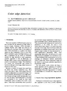
Figure 1: Most edge detectors make mistakes when (a) lowcontrast edges exist near high-contrast edges, or (b) a region contains strong internal edges.

Introduction

With few exceptions, the fundamental assumption of all step edge detectors is that the regions on either side of an edge are constant in color or intensity. Much effort has gone into making them robust to noise, but the noise is assumed to have statistically simple properties. Convolution masks are ideal for realizing this assumption because the sign of the weight at a pixel tells us what side of the edge it is hypothesized to be on. We can think of a convolution as finding the weighted mean of each side and then computing the distance between the two means. Using additional convolution masks, Wang and Binford [13] were able to find edges when shading caused regions to match a more general intensity surface. While this assumption holds well enough for many applications, it does not hold in all cases. For instance, as scale increases, it is more likely that the weighted mean of each side will not be meaningful because an operator will include image features unrelated to the edge. This observation is even more true of color images. When only intensities are involved, the average over a large window is still perceptually meaningful because intensities are totally ordered. In color images, there is no such ordering, so the “mean color” of a large window may have little perceptual similarity to any of the colors in it. Figure 1 shows two examples where the traditional assumptions do not hold. In Figure 1(a) the curved helmet of a statue occludes a complex background containing light

and dark regions. Though the two dark regions have a noticeable edge between them, the contrast is smaller than that between the light and dark regions. At the two corners near the center, the high-contrast edges’ responses will suppress the low-contrast edge’s response, and the true boundary will be lost. Increasing the scale parameter will eventually recover the edge, but other important edges will disappear. Only two regions are present in Figure 1(b), but the texture on the right contains both strong edges and the color of the region on the left. Though the boundary between the two regions is salient over a wide range of scales, not all edge detectors can distinguish it from the intra-texture edges at all scales. We propose an edge model that assumes that the two distributions of pixel values on either side of an edge are different. Distributions allow for more control over how each region is represented and how the distance between two regions is computed than can be achieved by using only the mean value. Besides handling the two cases of Figure 1, this edge model has other advantages. The first is a lack of false negatives compared to other models (e.g., Hueckel [4] and Nalwa-Binford [6]). According to Nalwa [5], false negatives result from a failure to “take into account all possible intensity variations that might accompany a step edge in practice” (p. 103). Since we use distributions, almost all of these variations are modeled implicitly. Inhomogeneities

can be uncorrelated (due to noise) or correlated (due to texture) without affecting performance. The second benefit is that using distributions creates a unifying framework for edge detection in binary, greyscale, color, or multi-spectral images, so long as a meaningful ground distance is defined. To place this model and the resulting edge detector in perspective with other color edge detectors, we briefly review the literature, which we divide into three categories: output fusion methods, multi-dimensional gradient methods, and vector methods. Output fusion methods perform greyscale edge detection on each color channel and combine the results into a single edge map. Alberto Salinas et al. [1] typify this method, using regularization to constrain the edge map to one that matches the data well and has minimum curvature at all points. Nevatia’s extension of the Hueckel operator [8] also falls into this category. Multi-dimensional gradient methods use all three channels to compute a single gradient. Di Zenzo [3] gives formulas for computing the magnitude and direction of the gradient (which, for color images, is a tensor) given the directional derivatives in each channel. There are two notable methods that process each pixel’s color as a vector. Yang and Tsai [15] perform bi-level thresholding on 8  8 blocks to find the best 3-D projection axis to convert each block to greyscale. Trahanias and Venetsanopoulos [12] use vector order statistics to compute a variety of measures for edge detection. In general, though, most color edge detectors do not treat a pixel’s color as a point in a color space, opting instead to decompose it into three separate values and combine them later. This is the natural result of starting with a greyscale edge detector, which usually makes explicit use of the fact that an image is a function from 2 to to fit a surface to the data, and trying to ‘extend’ it to color. We do not believe that feature extraction in human visual systems proceeds by separately projecting colors onto three axes. Therefore, the whole notion of ‘extending’ a greyscale edge detector to handle color images is suspect. The operator we propose avoids this difficulty. Consider placing an idealized, circular “compass” at a point in the image, and, as the “needle” spins, computing a scalar measure of the difference between the distributions of pixel values on either side of the needle. The orientation producing the maximum difference is the edge’s direction, and the magnitude yields a measure of edge strength. Combined, the two form a vector quantity similar to a gradient. In the sense that it does not compute derivatives of the image function, this “compass operator” is similar to the SUSAN operator [11]. However, SUSAN assumes that the two regions are constant, and it uses the spatial distribution of pixels to determine edge strength and orientation. It

R R

was designed for greyscale images, though creating a color version would be straightforward. The compass operator uses a more general model, though, so it is able to compute a richer description of an edge. For example, the orientation of an edge is often uncertain because of curvature or other reasons; we can detect this phenomenon and measure the amount of uncertainty. More importantly, the compass operator assumes equal color distributions if we place the needle normal to an ideal step edge, which is true regardless of edge contrast or of the smoothness of the transition between the two sides. By measuring the minimum difference over all orientations, we can determine how well the image window fits our edge model. A high minimum value often indicates a junction where three or more edges meet. The rest of this paper is organized as follows: Section 2 describes the design of the compass operator, Section 3 compares it to a multi-dimensional gradient method, and we conclude in Section 4.

2

The Compass Operator

In this section we develop the compass operator for color images. We start with the creation of distributions in Section 2.1. Section 2.2 describes the perceptual distance between two color points, followed by Section 2.3, which does the same for two color distributions. Section 2.4 shows how edge information is extracted from our computation.

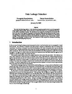
2.1 Creating Distributions A distribution of pixel colors on one side of an edge is represented as a color signature, a set of point masses in a color space [10]. The size of each point mass is determined by a weighting function that assigns a positive number to each pixel, and the number of point masses is determined by the complexity of the data. The pixels that comprise the two distributions used in each application of the operator are specified by the length, orientation, and position of a hypothesized edge; doing so creates a circle split into two semicircles with the edge as the diameter. There are two parts to the weighting function used to define the mass contributed by each pixel to each region: a “member” function whose value is equal to the area of a pixel (modeled as a square of unit area) inside the region, and a function that approaches zero as we move radially outward. The final weight is the product of the two values at each pixel. We take for granted Canny’s analysis of the onedimensional step edge that led to his optimal edge detector [2] and that the derivative of a Gaussian is a close approximation. In order to make all the mask weights positive, however, we flip the negative side of the function (Figure 2(a)). Instead of adding one side to the other, as is done in convolution, we instead compute a distance between the two signatures.

(a)

(b)

Figure 2: Weighting functions. (a) The Canny operator in 1-D. The negative side has been “flipped” so that all weights are positive. (b) Our weighting function, a surface of revolution of (a). Canny’s extension of his operator to two dimensions was motivated by computational considerations, as is our extension. We create an isotropic weighting function by forming a surface of revolution, as shown in Figure 2(b). In polar coordinates, it is written as f (r) = cr exp(;r 2 =22 ), where c is a normalizing constant and  is the scale parameter. The radius of the circle is 3. Using an isotropic weighting function makes it easier to compute distance values for all orientations because the mass that each pixel contributes remains constant. Furthermore, we sample the set of edge orientations uniformly, breaking the circle into wedges and allowing efficient updating of the signatures. The number and location of the point masses must still be determined. In theory, every distinct triple of color values could become a separate point mass, but this is prohibitively expensive, and for small radii the operator will suffer from overfitting. Vector quantization reduces the number of colors while retaining the modes of the distribution. Each image window is quantized once. We use the binary split algorithm of Orchard and Bouman [9], because it was developed for color images and allows control over the maximum codebook size. It is a greedy, tree-based algorithm that, at each step, takes the cluster whose covariance matrix contains the largest principal eigenvalue and splits it with a plane that is normal to the corresponding eigenvector and runs through the cluster’s mean. We could simply use histograms, which are a subset of signatures, but we do not wish to partition color space independently of the data. The maximum size of the codebook should be proportional to the value of . However, if an image window contains only a few colors, the signature need not have the maximum size. Therefore, our version of the binary split algorithm terminates early if the largest eigenvalue over all the clusters becomes too small.

2.2 A Perceptual Ground Distance Before defining the distance between two color signatures, we must first define the ground distance between two

colors. Because this distance should conform well to human perceptual distance as measured by psychophysicists, we use the CIE-Lab color space, in which small Euclidean distances are perceptually accurate [14]. If two colors are separated by a long distance, however, that distance is no longer quantitatively meaningful; the most we can say about the colors is that they are different. Using the Euclidean distance by itself presumes that an edge with a contrast of 80 units is twice as salient as an edge with a constrast of 40 units, which need not be true. We desire a distance measure that approaches but does not exceed 1 once the colors are far enough apart. There are many functions that satisfy this criterion, and we have chosen dij = 1 ; exp(;Eij = ); where Eij is the Euclidean distance between color i and color j and is a constant that determines the steepness of our function. We have empirically chosen = 14:0 for our experiments. It could be argued that such a measure is unnecessary, because edges are ultimately detected using a threshold, and we can set it to a lower value to detect edges of lower contrast. However, it is vital that this information regarding contrast is incorporated before the direction and strength of the edge are computed, not after. Otherwise, when edges of high and low contrast appear in the same window, the higher-contrast edge will suppress the response to the lower-contrast edge.

2.3 The Earth Mover’s Distance By dividing the circle in half, we have created two color signatures of equal mass, which we denote S1 and S2 . Finding the distance between them can be seen as an instance of the transportation problem (see [7]), in which we wish to find the minimum amount of physical work needed to move the masses of S1 into correspondence with those of S2 in color space. The Earth Mover’s Distance (EMD) [10] is based on a solution to this problem. It has been proven to be more robust than other distance measures when comparing the color signatures of entire images because it avoids many quantization and discretization artifacts. Given dij , the ground distance between every pair (i; j ) of colors, where color i is in S1 and color j is in S2 , the EMD finds a set of flows fij that minimizes

XX

dij fij ;

i2S1 j 2S2

subject to constraints ensuring that all the mass is moved from S1 to S2 . By normalizing the total mass of each signature to be 1 and choosing a ground distance that never exceeds 1, the EMD will always lie in [0, 1], regardless of scale.

1

0.8

EMD

0.6

0.4

0.2

0

0

50

100 Orientation

150

100 Orientation

150

f ()

Ideal Step Edge 1

0.8

EMD

0.6

0.4

0.2

0

Real Step Edge

0

50

f ()

Figure 3: Plots of EMD vs. orientation for ideal and real step edges. The EMD has two useful properties besides its robustness. First, it is a true metric, because our ground distance is a metric and the total mass of the signatures is equal. Also, it is a linear programming problem, so efficient algorithms are available.

2.4 Computing Edge Information We can now summarize the algorithm. Having computed the color signature of each wedge of the circle, the compass operator computes the EMD between the color signatures of every pair of semicircles formed by aggregating half the wedges together. The resulting EMD’s can be represented as a (periodic) function f (), 0   < 180 . The last step is to extract edge information from this function. The top row of Figure 3 shows the compass operator on an ideal step edge; f () is one period of a triangular wave. We define the orientation at the center point to be ^ = arg max f (), 90 in the example, and the strength to be f (^), which is 1 in this case. Note, however, that f () is sampled. To find the orientation and strength of an edge in general, we fit a parabola to the maximum point and the points on either side of it; the location of the vertex yields both values. In general, the image data may not be ideal for a number of reasons: (1) the edge could be blurred, (2) the two sides could share some color(s), (3) the center of the compass might be near but not on the edge, (4) the edge might be curved with respect to the chosen scale (including being part of a corner), or (5) the center could be near a junction where three or more edges meet. Many of these reasons are illustrated in the bottom example of Figure 3. Reasons (1) and (2) affect the strength but not the orientation. Blurring and overlap both cause partial correspon-

dence between the signatures, lowering the EMD. The other three causes are more problematic in that the edge orientation is uncertain. Many orientations may yield either the same pair of color signatures or merely the same EMD, and f () will contain a “maximum plateau” rather than a single maximum. There is no best way to determine the existence of a plateau empirically; we find the largest interval [a; b] that contains ^ (the orientation yielding the maximum EMD) and in which all EMD’s for orientations in [a; b] are above a threshold. This threshold is expressed as cf (^) ; d, where c  1 and d  0 are constants, so that it becomes tighter for higher strengths. If the width of this interval is no bigger than the orientation sampling interval (i.e. one or two samples are above threshold), fitting a parabola will give accurate strength and orientation information. If it is larger, we define the orientation to be the midpoint of the plateau, the strength to be the maximum EMD, and the uncertainty to be the width of the plateau. While the importance of the maximum is intuitive, the minimum is equally important. Regardless of strength, the minimum may still be zero if there is an orientation that produces two equal color signatures. The minimum measures the photometric symmetry of the data; when it is high, our edge model is violated. For this reason, the value min f () is called the abnormality. One cause of high abnormality is the existence of a junction. To illustrate this point, consider a pathological case where the circle encompasses k equal-size wedges meeting at the center, and each wedge is perceptually different from all others. Simple geometry shows that if k is odd, f () = (k ; 1)=k, and if k is even, f () contains k=2 periods of a triangular wave that varies between (k ;2)=k and 1. It is interesting to note that if the image data is odd symmetric with respect to the center of the circle (a checkerboard being the simplest case), then at the junctions, the EMD is zero at all orientations. Figure 4 shows three regions (white, blue, and black) meeting in a T-junction, with the strength and abnormality of each point shown as an intensity. A small gap in the strength occurs near the junction, which would likely result in the two edges being disconnected. The peak in the abnormality (the maximum value over all the minima) indicates the junction’s location. The notion of abnormality is important conceptually because it supports Wang and Binford’s claim that the direction of an edge is not always normal to the image gradient. When abnormality is high, the difference between the gradient direction and the edge normal is likely to be large. However, we do not advocate using abnormality to detect junctions directly because localization is dependent on

Image

Strength

Abnormality

Figure 4: When an image contains a junction, the strength of one of the edges invariably drops as it approaches, resulting in a gap. The abnormality (normalized for display) peaks near the junction’s location. the colors found in the region. If, unlike in Figure 4, two of the regions share some color, the junction will be displaced, and it will move as scale increases. Single corners cannot be detected because they have an axis of symmetry, resulting in no abnormality.

3

Edge Detection at Multiple Scales

There are three main advantages to the compass operator: the use of variable-length descriptions, which contain more information about a region than the weighted mean; the computation of EMD as a function of orientation, which ensures accurate orientation estimates while simultaneously providing uncertainty and abnormality information; and a saturating distance function, which removes the bias toward high-contrast edges. We now show a set of examples making clear the effect of these advantages by comparing the compass operator to a multi-dimensional version of Canny’s method [2]. The gradient is computed in a manner similar to that of Di Zenzo [3], by convolving each CIE-Lab color channel with a Gaussian derivative and combining the components into a single gradient vector. In the top left corner of Figure 5, the helmet of a statue occludes a brick wall, with a window sill casting a shadow. The shadow and the helmet are different shades of dark grey, but their contrast is minimal compared to the adjacent bricks and window sill. The four middle columns show, for  = 1, 4, 8, and 16, the gradient magnitude and extracted edges. The low-contrast boundary cannot be recovered using Canny’s method unless we are willing to sacrifice the outline of the window sill altogether. The compass operator, however, detects all of the important boundaries, as shown in the last column of Figure 5. In addition, the two maxima in the abnormality output (bottom left corner) show approximate locations of the two junctions where the shadow meets the helmet. The boundary between the two regions in Figure 6 is salient at a wide range of scales. As we track this edge through scale space, however, we see that Canny’s method makes a mistake at  = 8 and connects an intra-texture

edge to the boundary. The mistake is eventually corrected, but the edge at  = 16 has a curve and is, therefore, not well localized. The compass operator’s output is stable throughout. Our final example shows edges extracted by each method over a large 320160 image from which Figure 5 was taken. Figure 7(c) shows the edges detected by Canny’s method, while Figure 7(d) shows the compass operator’s edges. The difference between the two is very apparent, especially in the figure’s helmet, shield, right arm, and legs. The compass operator produces smaller gaps between edges and retains more of the actual boundary of the statue. Furthermore, the abnormality (Figure 7(b)), a quantity Canny’s edge detector cannot produce, shows a number of places where we might look to link edges together into junctions. One area where the gradient magnitude is demonstrably better than the compass operator strength is in computation time. Canny’s edge detector can process an entire image in seconds, while the compass operator’s time varies from 24,000 pixels per minute for  = 2 to 5,000 pixels per minute for  = 16 on an SGI Indigo 2. To improve the running time, we suggest sampling the image spatially every =2 pixels and interpolate the intermediate values, which produces only minor degradation. One could also use cruder vector quantization methods, such as histogramming, and a cruder distance measure instead of the EMD, but the quality of the results is likely to suffer greatly.

4

Conclusion

The compass operator substitutes vector quantization and the Earth Mover’s Distance for Gaussian smoothing and taking derivatives. The resulting framework is applicable to any image range, with the only changes being the dimensionality of the data and the ground distance between two values. The model is powerful enough to detect edges that Canny’s edge detector cannot, and it remains more stable as scale varies. Uncertainty in the edge orientation can also be computed, as well as a rough estimate of the location of junctions. We have identified the stability of a pixel’s representative after vector quantization as a key issue. Because all windows are treated independently, a pixel can conceivably be mapped to different colors. This instability can cause gaps or even the loss of entire edges. An interesting observation is that the principles behind the operator can be applied to any zero-mean convolution mask. Potentially, the need for color images to require three times as many filters as a greyscale image could be eliminated, as could the need for correlation functions between different color channels. Another intriguing extension of our work is to combine the wedges of the circle asymmetrically, creating a corner

——– Multi-Dimensional Gradient Magnitude ——– (Di Zenzo [3] and Canny [2])

Image

Compass Abnormality

=1



=4



=8

 = 16

Compass Strength



=4

——————– Edges extracted from the above images ——————– (Non-maximal suppression and thresholding)

Figure 5: The shadow cast by the window sill causes the helmet of a statue to have both high- and low-contrast edges. No value of  allows the Canny operator to detect all the relevant edges that the compass operator does. The bright spots in the abnormality image indicate two junctions in the vicinity. The gradient magnitude images are normalized. Edges found using the Canny Edge Detector

Image

=2



=4



=8

 = 16

Edges found using the Compass Operator Figure 6: The main edge in this image is salient at a large range of scales even though one side is heavily textured. Canny’s edge detector makes an error by  = 8, and the lone edge at  = 16 is curved. The compass operator is stable throughout scale space.

(a)

(b)

(c)

(d)

(e)

Figure 8: (a) An ideal corner. (b) Compass operator strength. (c) Magnification of (b); the corner point (center) is not a maximum in any direction. (d) 90 corner detector strength. (e) Magnification of (d); the corner point is a local maximum.

detector that computes the EMD between color distributions of unequal mass. In Figure 8, we compare the edge strength of the compass operator to the corner strength of a 90 corner detector based on the same principles. Future work will focus on these extensions, along with the integration of edges, corners, and junctions.

Acknowledgement We thank Yossi Rubner for providing the EMD code.

References [1] R. Alberto Salinas, C. Richardson, M.A. Abidi, and R.C. Gonzalez. Data fusion: Color edge detection and surface reconstruction through regularization. IEEE Trans. on Ind. Elec., 43(3):355–363, June 1996. [2] J. Canny. A computational approach to edge detection. PAMI, 8(6):679–698, November 1986. [3] S. Di Zenzo. A note on the gradient of a multi-image. CVGIP, 33(1):116–125, January 1986. [4] M. Hueckel. An operator which locates edges in digitized pictures. JACM, 18(1):113–125, January 1971. [5] V.S. Nalwa. A Guided Tour of Computer Vision. AddisonWesley, Reading, MA, 1993.

(a) Image

(b) Abnormality

[6] V.S. Nalwa and T.O. Binford. On detecting edges. PAMI, 8(6):699–714, November 1986. [7] A.D. Nering and A.W. Tucker. Linear Programs and Related Problems, chapter 9. Academic Press, 1993. [8] R. Nevatia. A color edge detector and its use in scene segmentation. IEEE Trans. on Sys., Man, and Cyb., 7(11):820– 826, November 1977. [9] M.T. Orchard and C.A. Bouman. Color quantization of images. IEEE Trans. on Signal Proc., 39(12):2677–2690, December 1991. [10] Y. Rubner, C. Tomasi, and L.J. Guibas. A metric for distributions with applications to image databases. In ICCV98, pages 59–66, January 1998. [11] S.M. Smith and J.M. Brady. Susan: A new approach to low-level image-processing. IJCV, 23(1):45–78, May 1997.

(c) Canny

(d) Compass Operator

Figure 7: Comparison of edges on a 320  160 image. Note the differences in the helmet, shield, right arm, and legs. The peaks in the abnormality (b), normalized for display, indicate potential junctions. Both algorithms were run using  = 4.

[12] P.E. Trahanias and A.N. Venetsanopoulos. Vector orderstatistics operators as color edge detectors. IEEE Trans. on Sys., Man, and Cyb.-B, 26(1):135–143, February 1996. [13] S.-J. Wang and T.O. Binford. Generic, model-based estimation and detection of discontinuities in image surfaces. In Image Understanding Workshop, volume II, pages 113–116, November 1994. [14] G. Wyszecki and W.S. Stiles. Color Science: Concepts and Methods, Quantitative Data and Formulae. John Wiley and Sons, New York, NY, 1982. [15] C.K. Yang and W.H. Tsai. Reduction of color space dimensionality by moment-preserving thresholding and its application for edge-detection in color images. Pattern Rec. Letters, 17(5):481–490, May 1996.