to perform corner detection on color images whose re- gions contain texture. We show ... The next two sections explain the region and edge models, respectively ...
In IEEE Seventh International Conference on Computer Vision, Volume 2, pages 1039-1045, September 1999
Corner Detection in Textured Color Images Mark A. Ruzon
Carlo Tomasi
Computer Science Department Stanford University Stanford, CA 94305
Abstract
Corner models in the literature have lagged behind edge models with respect to color and shading. We use both a region model, based on distributions of pixel colors, and an edge model, which removes false positives, to perform corner detection on color images whose regions contain texture. We show results on a variety of natural images at di�erent scales that highlight the problems that occur when boundaries between regions have curvature. 1
Introduction
Corners and junctions (multiple corners at the same image location) are crucial for high-level vision tasks because they represent occlusions useful to stereo and motion algorithms, and they provide shape information for object recognition. They are arguably at least as important as edges, yet current edge models invoke fewer assumptions and are more robust than current corner models. Speci cally, edge models proposed in the literature are superior to existing corner models with respect to color and shading. Many color edge detectors have been proposed ([1], [5], and [11] form a representative sample), but corner detectors have been con ned to greyscale images. Certain algorithms (e.g. [8]) appear to be easily extendable to color images. The e�ects of shading on the direction of the image gradient were modeled by Wang and Binford [12] to create an edge detector insensitive to shading, while most corner detectors assume that regions are of constant intensity (Alvarez and Morales [2] assumed level sets). Many corner detectors start with an edge map rather than an image (e.g. [6] and [7]), which would appear to mitigate such e�ects. However, we argue against using these indirect methods for two reasons: (1) using the output of an algorithm whose goal is something other than corner detection causes unknown biases and errors to propagate into the corner detector, and (2) the analysis of Deriche and Giraudon
[4] showed that edges found by rst-derivative operators tend to \round o�" corners. Without using the image itself, it is impossible to distinguish true corners from curved boundaries. Therefore, we opt for a direct approach. At a conceptual level, corner and edge detection algorithms both compute the degree to which two adjacent regions are dissimilar. Corners do not bisect an operator's support, however, and the resulting asymmetry must be accounted for. Also, corners are point features, so only one response to the same part of the image can be accepted. Detecting junctions, though, requires accepting multiple responses of the corner detector in the same or nearly the same image location. Our approach uses both a region model, from which we create a set of corner candidates, and an edge model, which decides whether to accept or reject a candidate. We model a corner as two adjacent regions that di�er in their color distributions. The resulting operator generalizes edge detection to asymmetric regions with multiple colors per region. Multiple colors are represented by a set of point masses in a color space. The distance between two such sets is found using the Earth Mover's Distance, which measures the minimumamount of \work" required to transform one set into the other in that space. The advantage of this model is that we can detect corners (and edges, see [10]) in textured regions where other detectors cannot. Two textures may have the same \mean color," for example, even though they have no color in common. Furthermore, the texture need not be homogeneous as long as its colors are suf ciently di�erent from its neighbors. An edge model is also necessary, because corners cannot exist independently of edges. Our model, inspired by Deriche and Giraudon's, presumes that at the two endpoints of the corner, there is a strong edge response in the same direction. Furthermore, the edge response between the two endpoints of the corner should be weaker than the corner response. We can
A
B
R (x,y)
α
SO SI
θ
(a)
(b)
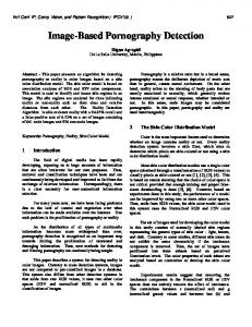
Figure 1: Parts of the region model. (a) Illustration of operator parameters. (b) The pixel weighting function, a surface of revolution of half of a Gaussian derivative function. compare corner candidates with this model to exclude most false positives in the operator's response. If multiple candidates all respond well to the same corner, we group them and choose the \best" candidate. The next two sections explain the region and edge models, respectively, after which we present the results and our conclusions. 2
The Region Model
In this section we develop a model of two adjacent regions and the perceptual distance between them. In Section 2.1 we summarize the representation of a region as a color signature; details are in [10]. Section 2.2 tackles the problem of asymmetry between the two regions, and Section 2.3 explains how initial corner candidates are selected.
2.1 Color Signatures
A color signature is a set of point masses that represents one of the two regions. There are ve parameters that determine which pixels will belong to each region: (x; y), the location of the center of the window; � 2 [0; 360), the orientation of the corner (de ned as the angle formed by the positive x-axis and the \clockwise" side of the corner); � 2 (0; 180], the angle subtended by the corner; and R, the scale parameter (Figure 1(a)). Because it is natural to consider a corner as a wedge, the window is a circle of radius R. Vector quantization applied to the circle determines the number and location of the point masses. Each pixel contributes a weight dependent only on its distance to the center. The polar function f (r) = r2 ; 2 2 � cre , where c is a normalizing constant and � = R=3, is the positive half of a 1-D Gaussian derivative function revolved around the y-axis (Figure 1(b)). Isotropy simpli es computations over all combinations of � and � because the mass that each pixel contributes remains constant. Sampling the ranges of � and �
partial
A B
SI 1 SO 1
EMD: 0
0 6
normalized
A B SI 1 0 SO 1=7 6=7 EMD: 6=7
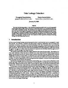
Figure 2: The normalized EMD can detect corners that the partial EMD cannot. equally breaks the circle into wedges, allowing e�cient updating of the signatures. We use 15� wedges. We represent colors in the CIE-Lab color space [13], in which short, Euclidean distances are perceptually accurate. To account for the fact that long distances are not, we use a normalized measure that saturates: dij = 1 ; exp(;Eij = ); where Eij is the Euclidean distance between color i and color j , and = 14:0 is a constant determining the steepness of the function. The distance between two color signatures is found using the Earth Mover's Distance (EMD) [9]. The EMD measures the minimumamount of physical work needed to move the masses of one signature into correspondence with the other. In our formulation, the EMD lies in [0, 1] since the maximum amount of mass that can be moved and the maximum distance it can move are both 1.
2.2 Partial EMD vs. Normalized EMD
After creating two color signatures, SI inside the corner and SO outside it, we can use the EMD to measure the similarity between the two regions. An important issue in this computation that is not present when using this model for edge detection is that SO always has more mass than SI . We normalize SI to have a mass of 1, regardless of the value of �, to preserve the same output range. There are two ways to normalize SO : we can use the same constant and nd the EMD between signatures of unequal mass (\partial" EMD), or we can assign SO a mass of 1 also (\normalized" EMD). Each type of EMD has di�erent advantages. In Figure 2 the normalized EMD detects a corner that the partial EMD does not. A 45� corner consists entirely of color A, while the oustide region has amounts of colors A and B (a perceptual distance of 1 from A) in
in natural images. For the corners that we do detect, it is best to describe them as accurately as possible.
B SO
1111 0000 0000 1111 0000 1111 S 0000 1111 0000A 1111
2.3 Finding Corner Candidates
I
30�
SI SO
partial
A
B
1 0 0.8 10.2 EMD: 0.2
60�
SI SO
partial
A
B
0.9 0.1 0 5
normalized
A
B SI 1 0 SO 0:07 0:93 EMD: 0.93
normalized
A B SI 0.9 0.1 SO 0 1
EMD: 0.9
EMD: 0.9
partial
normalized
The process of corner detection begins by measuring the EMD over all circular windows and for all combinations of � and �. The result is a list of threedimensional tensors, one for each value of �. Corner candidates are maximum values over x, y, and � that are above a threshold. Parabolic interpolation over � gives the actual strength and orientation of a candidate. Output for di�erent values of � cannot be compared directly, however, even though the range of values is the same. From a purely statistical standpoint, it is less likely that a large EMD will result from a smaller value of � because of the greater imbalance in the amount of mass. The net e�ect is that we must vary our threshold linearly with �. In addition, we must choose bounds on � because the output at small values is less reliable due to noise, and large corners are hard to distinguish from edges. We have chosen �min = 30� and �max = 150� . 3
Corner Detection
Figure 3: The partial EMD can more accurately describe a corner.
In this section, we present our edge model (Section 3.1) and consider the problem of pruning multiple responses to the same corner that all satisfy this model (Section 3.2).
a 1:6 ratio. We de ne the mass of SI to be 1, and the mass of SO can be either 1 or 7. If we choose the mass to be 7 (partial EMD), then SI becomes a subset of SO , and the distance is 0. If instead we choose the mass of SO to be 1 (normalized EMD), the distance is 6=7, and a corner is likely to be found. Figure 3 shows a situation where the partial EMD describes a corner more accurately than the normalized EMD. A 60� corner consists entirely of color A except for the two edges, which contain some pixels of color B . If 10% of the pixels inside the corner have color B , then the values of the EMD are those shown in the accompanying table. Both types of EMD detect a corner, but the normalized EMD estimates � to be 30� while the partial EMD correctly estimates � to be 60� . An example of the di�erences for real image data is shown below the table. The corner found by the partial EMD runs along the edges, while the other does not. We have chosen the partial EMD for our experiments. Although we may have false negatives, the number is likely to be small because the frequency of the phenomenon illustrated in Figure 2 is inversely proportional to �, and such corners are less frequent
In order for a true corner to exist, there must be evidence of strong edges that are consistent with the location, orientation, and angle of the corner. A basic schematic of our model is illustrated in Figure 4(a). Speci cally, our model incorporates three ideas: 1. Edge direction at each end of a corner must match the orientation of the side of that corner. 2. Edge response at each end of a corner must be high. 3. Between the two ends of a corner, the edge response must be weaker than the corner response. In theory, none of these conditions is satis ed when a corner candidate falsely responds to an edge (Figure 4(b)). Before we can measure the degree to which a corner matches our model, we must have edge information. This is found by applying our operator with � = 180�, and nding the orientation at each image location that maximizes the response (see [10] for details). Once this is done, we nd two angles: �C , the di�erence in orientation between the clockwise side of the
3.1 The Edge Model
(a)
(b)
Figure 4: (a) A true corner. The edge is aligned with the corner at the endpoints and \rounded o�" in the middle, where the response weakens. (b) A false positive due to inhomogeneities on one side of an edge. corner and the edge response at the corner's endpoint, and �CC , the corresponding angle for the counterclockwise side. Because edges have two valid orientations (di�ering by 180�), we choose the one that yields the smaller angle. Our measurement P can be expressed as P = cos �C + cos �CC ; which lies between 0 and 2. We threshold P at 1.97. Finally, where the edge crosses the line that bisects the corner, the projection of the edge response onto the line normal to the bisector must be weaker than the corner response. We check responses on a small interval along the bisector line centered at a point R(sec �2 ; tan �2 ) pixels away from the corner. This quantity is the distance from the corner point to the circumference of an imaginary circle tangent to the sides of the corner at its endpoints. Applying all three parts of the model to the set of initial corner candidates greatly reduces their number. Figure 5(a) shows the candidates for an image patch consisting of cut stone against an ivy-covered wall. Though all the candidates are near the boundary between the two regions, most of them do not t the boundary well. Figure 5(b) shows the results after applying the edge model.
3.2 Pruning Multiple Responses
Using edge data, however, does not completely solve our problem. Figure 5(b) contains two corners, each of which gives a strong corner response to the same area of the image and matches the edges well. Obviously, we would like to have only one. The question of which corners to group together in this image is trivial, but the general question of when two or more corners are \close enough" to each other that one should be accepted and the rest rejected has no de nitive answer in natural images. We de ne two corners as being \close enough" if the corner points are within 3R=4 pixels of each other
(a)
(b)
(c)
Figure 5: Corner detection steps applied to operator output of cut stone occluding an ivy-covered wall. (a) Initial corner candidates. (b) After applying the edge model. (c) Final result after pruning multiple responses. and one of the following conditions is true: (1) the two clockwise orientations di�er by no more than 10�, (2) the two counterclockwise orientations di�er by no more than 10�, or (3) the sum the di�erences is no more than 40� . These conditions group \nested" corners while preserving multiple corners near junctions. An ambiguity arises when corner X is close to corners Y and Z , but Y and Z are not close to each other. If our notion of \closeness" is global, then the order in which we examine corners a�ects the nal output. Since this is unacceptable, we compute the transitive closure of \closeness," that is, X , Y , and Z will all become part of the same set. It is theoretically possible that corners in distant parts of the image could become part of the same set; in practice, however, the application of the edge model removes enough candidates that this does not happen often. Once we have computed the transitive closure, we pick the member of each set that maximizes the expression 2C + P + E , where C is the corner response, P is the degree of orientation match described earlier, and E is the sum of the edge responses at the endpoints of the two sides of the corner. C is doubled so that each term contributes equally. The nal corner of our example is shown in Figure 5(c). 4
Results
In this section we present results on a variety of image patches in order to convey the versatility of the operator. All the results in this paper that use the partial EMD were computed with the same thresholds. The lengths of the sides of the corners in the images are equal to the chosen value of R. Color versions of the results are available from http://vision.stanford.edu/public/publication/. Figure 6 shows one fabric occluding another. Al-
Figure 7: Corners found between three regions.
Figure 6: Two fabrics. Note the heterogeneity of each texture, as well as the existence of shadows. though each contains texture that varies greatly in color and has regions in partial shadow, the corner is correctly detected. Figure 7 is more complicated because three textures are involved: trees (upper left), rock (lower left), and rock in deep shadow (right). Five corners are found that separate the regions and, incidentally, form most of the boundary of the illuminated rock. In Figure 8 we show output at three di�erent scales. The image contains a junction, but the textured region subtends an angle greater than �max , and the region boundaries are not rays emanating from the junction. At all three scales we nd the two smaller corners with compatible orienations and corner points near each other. We emphasize that corners are estimated independently; a true junction detector would combine these corners, perhaps with knowledge of the lack of symmetry near the junction [10], to estimate its location and parameters. Other researchers have examined the evolution of corners across scales in more detail. Mokhtarian and Suomela [7] detected corners at a large scale and used smaller scales to localize them, an approach that might work well here. Alvarez and Morales' framework [2] caused corners to evolve along the line bisecting the corner. Their framework depends on the level set as-
sumption, which is violated here. Neither appears to have been tested on boundaries with continuously changing curvature or on corners as large as 150�, though. Finally, we wish to mention the running time. The operator is implemented in C and can process image locations (each including all combinations of � and �) at a rate on the order of 1500 per minute on an SGI Indigo 2, depending on R. 5
Conclusion
We have presented an operator that outputs high values when two regions inside and outside of a corner have di�erent color distributions. Using color signatures and the Earth Mover's Distance allows us to detect corners in situations that others have not even considered because they are forced to assume that each region is constant. The edge model eliminates those corners that are not supported by evidence of strong edges. This basic dependence of corners on edges is both conceptually important and practically e�ective. The application of corner detection to natural images that are not composed mostly of polygons brings up many interesting issues, the most important of which is the de nition of a corner. We have not speci ed an optimality condition from which our operator can be derived, because deciding that a corner exists is mostly a question of thresholding the curvature of an edge with respect to the chosen scale. By the same token, there is no ground truth in natural images to compare our results to. The results are best evaluated
Figure 9: A rock with edges (black) and corners (white) drawn. The features are complementary. in the context of an application, such as tracking landmarks for robotic navigation or, more generally, shape recovery for object recognition. Another fundamental issue is the integration of corners and edges. One approach may be to detect them separately and use the corners to perturb the edges toward the true boundary. In Figure 9 we have drawn, in addition to the two corners, a set of edges found by thresholding and performing non-maximal suppression [3] on the operator's output at � = 180�. Through a suitable process (e.g. energy minimization), it may be possible to conform the edges to the corners and produce a more accurate boundary. However, the fact that we can compute edge and corner information in the same framework by changing the value of � begs the question of whether the two are fundamentally di�erent at all. It is unsatisfactory that we must exclude corners between 150� and 180�. In Figure 10 we have drawn both edges and corners, including � = 165�, on top of a natural image. The large amount of overlap indicates that the two di�erent algorithms are producing nearly the same output, though they do complement each other in a few places. Future research will investigate a boundary model in which both edges and corners can be detected and related to each other without creating an arti cial distinction between them.
Acknowledgment Figure 8: Comparison of output at three di�erent scales near a junction. One corner of the junction is greater than 150� and cannot be recovered directly.
We thank Yossi Rubner for the EMD code.
References [1] R. Alberto Salinas, C. Richardson, M.A. Abidi, and R.C. Gonzalez. Data fusion: Color edge detection and
Figure 10: Canyon with corners (left) and edges (right). Note the high amount of overlap. 165� corners have been included.
[2] [3] [4] [5] [6] [7]
surface reconstruction through regularization. IEEE Trans. on Ind. Elec., 43(3):355{363, 1996. L. Alvarez and F. Morales. A�ne morphological multiscale analysis of corners and junctions. IJCV, 25(2):95{107, 1997. J. Canny. A computational approach to edge detection. PAMI, 8(6):679{698, 1986. R. Deriche and G. Giraudon. A computational approach for corner and vertex detection. IJCV, 10(2):101{124, 1993. S. Di Zenzo. A note on the gradient of a multi-image. CVGIP, 33(1):116{125, 1986. Q. Ji and R. Haralick. Breakpoint detection using covariance propagation. PAMI, 20(8):845{851, 1998. F. Mokhtarian and R. Suomela. Robust image corner detection through curvature scale space. PAMI, 20(12):1376{1381, 1998.
[8] L. Parida, D. Geiger, and R. Hummel. Junctions: Detection, classi cation, and reconstruction. PAMI, 20(7):687{698, 1998. [9] Y. Rubner, C. Tomasi, and L.J. Guibas. A metric for distributions with applications to image databases. In ICCV98, pages 59{66, 1998. [10] M. Ruzon and C. Tomasi. Color edge detection with the compass operator. In CVPR99, volume 2, pages 160{167, 1999. [11] P.E. Trahanias and A.N. Venetsanopoulos. Vector order-statistics operators as color edge detectors. IEEE SMC-B, 26(1):135{143, 1996. [12] S.-J. Wang and T.O. Binford. Generic, model-based estimation and detection of discontinuities in image surfaces. In ARPA IUW, volume II, pages 113{116, 1994. [13] G. Wyszecki and W.S. Stiles. Color Science: Concepts and Methods, Quantitative Data and Formulae. John Wiley and Sons, New York, NY, 1982.