Color Histogram Features Based Image Classification in Content ...

Color Histogram Features Based Image Classification in Content-Based Image Retrieval Systems Szabolcs Sergyán Budapest Tech John von Neumann Faculty of Informatics Institute of Software Technology Bécsi u´ t 96/B, Budapest, H-1034, Hungary [email protected] Abstract— In content-based image retrieval systems (CBIR) the most efficient and simple searches are the color based searches. Altough this methods can be improved if some prepocessing steps are used. In this paper one of the prepocessing algorithms, the image classification is analized. In CBIR image classification has to be computationally fast and efficient. In this paper a new approach is introduced, which based on low level image histogram features. The main advantage of this method is the very quick generation and comparison of the applied feature vectors.

I. I NTRODUCTION In content-based image retrieval systems (CBIR) [3] is very useful and efficent if the images are classified on the score of particular aspects. For example in a great database the images can be divided into such classes as follows: landscapes, builidings, animals, faces, artifical images, etc. Many color image classification methods use color histograms. In [5] feature vectors are generated using the Haar wavelet and Daubechies’ wavelet of color historgrams. Another histogram based approach can be found in [1], where the so-called blobworld is used to search similar images. The aim of this paper to develop such a color histogram based classification approach, which is efficient, quick and enough robust. In the interest of this I used some features of color histograms, and classified the images using these features. The advantage of this approach is the comparison of histogram features is much faster and more efficient than of other commonly used methods. In Section 2 the theoretical background of my approach is introduced. In Section 3 the experiments can be found, and in Section 4 I wrote the conclusions and possible further works. II. T HEORETICAL BACKGROUND Hereinafter I summarize the theoretical background of my classification method. The certain subsections are based on [4]. A. Histogram Features The histogram of an image is a plot of the gray level values or the intensity values of a color chanel versus the number of pixels at that value. The shape of the histogram provides us

978-1-4244-2106-0/08/$25.00 © 2008 IEEE.

with information about the nature of the image, or subimage if we are considering an object within the image. For example, a very narrow histogram implies a low contrast image, a histogram skewed toward the high end implies a bright image, and a histogram with two major peaks, called bimodal, implies an object that is in contrast with the background. The histogram features that we will consider are statisticalbased features, where the histogram is used as a model of the probability distribution of the intensity levels. These statistical features provides us with information about the characteristics of the intensity level distribution for the image. We define the first-order histogram probability, P (g), as: P (g) =

N (g) M

(1)

M is the number of pixels in the image (if the entire image is under consideration then M = N 2 for an N × N image), and N (g) is the number of pixels at gray level g. As with any probability distribution all the values for P (g) are less than or equal to 1, and the sum of all the P (g) values is equal to 1. The features based on the first order histogram probability are the mean, standard deviation, skew, energy, and entropy. The mean is the average value, so it tells us something about the general brightness of the image. A bright image will have a high mean, and a dark image will have a low mean. We will use L as the total number of intensity levels available, so the gray levels range from 0 to L − 1. For example, for typical 8-bit image data, L is 256 and ranges from 0 to 255. We can define the mean as follows: g¯ =

L−1 X g=0

gP (g) =

X X I(r, c) r

c

M

(2)

If we use the second form of the equation we sum over the rows and columns corresponding to the pixels in the image under consideration. The standard deviation, which is also known as the square root of the variance, tells us something about the contrast. It describes the spread in the data, so a high contrast image will

221

SAMI 2008 • 6th International Symposium on Applied Machine Intelligence and Informatics

have a high variance, and a low contrast image will have a low variance. It is defined as follows: v uL−1 uX 2 σg = t (g − g¯) P (g) (3) g=0

The skew measures the asymmetry about the mean in the intensity level distribution. It is defined as: SKEW =

L−1 1 X 3 (g − g¯) P (g) σg3 g=0

(4)

The skew will be positive if the tail of the histogram spreads to the right (positive), and negative if the tail of the histogram spreads to the left (negative). Another method to measure the skew uses the mean, mode, and standard deviation, where the mode is defined as the peak, or highest, value: SKEW ′ =

g¯ − mode σg

(5)

This method of measuring skew is more computationally efficient, especially considering that, typically, the mean and standard deviation have already been calculated. The energy measure tells us something about how the intensity levels are distributed: EN ERGY =

L−1 X

C. Distance and Similarity Measures 2

[P (g)]

(6)

g=0

The energy measure has a maximum value of 1 for an image with a constant value, and gets increasingly smaller as the pixel values are distributed across more intensity level values (remember all the P (g) values are less than or equal to 1). The larger this value is, the easier it is to compress the image data. If the energy is high it tells us that the number of intensity levels in the image is few, that is, the distribution is concentrated in only a small number of different intensity levels. The entropy is a measure that tells us how many bits we need to code the image data, and is given by EN T ROP Y = −

L−1 X

feature and assign a number to it, it becomes a numerical feature. Care must be taken is assigning numbers to symbolic features, so that the numbers are assigned in a meaningful way. For example with color we normally think of the hue by its name such as ”orange” or ”magenta”. In this case, we could perform an HSL transform on the RGB data, and use the H (hue) value as a numerical color feature. But with the HSL transform the hue value ranges from 0 to 360 degrees, and 0 is ”next to” 360, so it would be invalid to compare two colors by simply subtracting the two hue values. The feature vector can be used to classify an object, or provide us with condensed higher-level image information. Associated with the feature vector is a mathematical abstraction called a feature space, which is also n-dimensional and is created to allow visualization of feature vectors, and relationships between them. With two- and three-dimensional feature vectors it is modeled as a geometric construct with perpendicular axes and created by plotting each feature measurement along one axis. For n-dimensional feature vectors it is an abstract mathematical construction called a hyperspace. As we shall see the creation of the feature space allows us to define distance and similarity measures which are used to compare feature vectors and aid in the classification of unknown samples.

P (g) log2 [P (g)]

(7)

g=0

As the pixel values in the image are distributed among more intensity levels, the entropy increases. A complex image has higher entropy than a simple image. This measure tends to vary inversely with the energy. B. Feature Vectors and Feature Spaces A feature vector is one method to represent an image by finding measurements on a set of features. The feature vector is an n-dimensional vector that contains these measurements, where n is the number of features. The measurements may be symbolic, numerical, of both. An example of a symbolic feature is color such a ”blue” or ”red”; an example of a numerical feature is the area of an object. If we take a symbolic

The feature vector is meant to represent the object and will be used to classify it. To perform the classification we need methods to compare two feature vectors. The primary methods are to either measure the difference between the two, or to measure the similarity. Two vectors that are closely related will have a small difference and a large similarity. The difference can be measured by a distance measure in the n-dimensional feature space; the bigger the distance between two vectors, the greater the difference. Euclidean distance is the most common metric for measuring the distance between two vectors, and is given by the square root of the sum of the squares of the differences between vector components. Given two vectors A and B, where:     a1 b1  a2   b2      A =  .  and B =  .  (8)  ..   ..  an

bn

then the Euclidean distance is given by: v u n uX 2 t (ai − bi )

(9)

i=1

Another distance measure, called the city block of absolute value metric, is defined as follows (using A and B as above): n X

|ai − bi |

(10)

i=1

222


This metric is computationally faster than the Euclidean distance, but gives similar results. A distance metric that considers only largest difference is the maximum value metric defined by: max {|a1 − b1 | , |a2 − b2 | , . . . , |an − bn |}

(11)

We can see that this will measure the vector component with the maximum distance, which is useful for some applications. A generalized distance metric is the Minkowski distance defined as: "

n X

|ai − bi |

r

i=1

#1/r

(12)

where r is a positive integer. The Minkowski distance is referred to as generalized because, for instance, if r = 2 it is the same as Euclidean distance and when r = 1 it is the city block metric. The second type of a metric used for comparing two feature vectors is the similarity measure. Two vectors that are close in the feature space will have a large similarity measure. The most common form of the similarity measure is the vector inner product. Using our definitions for the two vectors A and B, we can define the vector inner product by the following equation: n X

ai bi

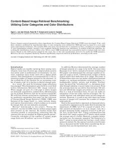
K = 5. Then we assign the unknown feature vector to the class that occurs most often in the set of K-Neighbors. This is still very computationally intensive, since we have to compare each unknown sample to every sample in the training set, and we want the training set as large as possible to maximize success. We can reduce this computational burden by using a method called Nearest Centroid. Here, we find the centroids for each class from the samples in the training set, and then we compare the unknown samples to the representative centroids only. The centroids are calculated by finding the average value for each vector component in the training set. III. E XPERIMENTS During the experiments 200 several images were used, which was divided into four equal size classes: landscapes, buildings, faces and indoor images with one object with homogenous background. One image of each class can be seen in Figure 1.

(13)

i=1

Another commonly used similarity measure is the Tanimoto metric, defined as:

n P

i=1

a2i +

n P

i=1 n P

i=1

ai bi b2i −

n P

(14) ai bi

i=1

This metric takes on values between 0 and 1, which can be thought of as a ”percent of similarity” since the value is 1 (100%) for identical vectors and gets smaller as the vectors get farther apart. D. Classification Algorithms and Methods The simplest algorithm for identifying a sample from the test set is called the Nearest Neighbor method. The object of interest is compared to every sample in the training set, using a distance measure, a similarity measure, or a combination of measures. The ”unknown” object is then identified as belonging to the same class as the closest sample in the training set. This is indicated by the smallest number if using a distance measure, or the largest number if using a similarity measure. This process is computationally intensive and not very robust. We can make the Nearest Neighbor method more robust by selecting not just the closest sample in the training set, but by consideration of a group of close feature vectors. This is called the K-Nearest Neighbor method, where, for example,

Fig. 1. Sample images of each class: landscape, building, face, indoor image with one object

From each image classes 25 images were the member of the training class. During the train period the YCbCr color space was applied, beacuse in an earlier paper [2] I analized which color space is the most efficient for classification, and this one was found. Using each training set the historgrams of the three color chanels were generated, and the abovementioned histogram features were calculated. Hence in each training set there were 25 pieces 15-dimensional feature vectors, which were made a 15-dimensional hyperspace. In these hyperspaces the Nearest Centorids were calculated as the class property using the absolute value metric. After the property generation of the training set I analized that the remaining 100 images are closest to which class. I found the 87% of images were well classified during the experiment. The algorithms were coded in MATLAB, because this system is computationally is rather fast, and the code generation is

223


very simple. For example the MATLAB code of the histogram feature generation can be seen in Figure 2. function t=HistogramProperties(PrH,N) t.m=sum([1:N]’.*PrH); t.s=sqrt(sum(([1:N]’-t.m).ˆ2.*PrH)); t.sk1=sum(([1:N]’-t.m).ˆ3.*PrH)/t.s.ˆ3; mode=find(PrH == max(PrH)); t.sk2=(t.m-mode(ceil(length(mode)/2)))/t.s; t.er=sum(PrH.ˆ2); t.ep=-sum(PrH.*log2(PrH+eps)); Fig. 2.

MATLAB code of the generation of histogram features

R EFERENCES [1] C. Carson, M. Thomas, S. Belongie, J.M. Hellerstein, J. Malik, “Blobworld: A System for Region-Based Image Indexing and Retrieval,” Third International Conference on Visual Information Systems, Springer, 1999. [2] Sz. Sergyán, “Color Content-based Image Classification,” 5th SlovakianHungarian Joint Symposium on Applied Machine Intelligence and Informatics, Poprad, Slovakia, pp. 427–434, 2007. [3] A.W.M. Smeulders, M. Worring, S. Santini, A. Gupta, R. Jain, “ContentBased Image Retrieval at the End of the Early Years,” IEEE Transactions on Pattern Analysis and Machine Intelligence, vol. 22, no. 12, pp. 1349– 1380, 2000. [4] S.E. Umbaugh, “Computer Imaging – Digital Image Analysis and Processing,” CRC Press, 2005. [5] A. Vadivel, A.K. Majumdar, S. Sural, “Characteristics of Weighted Feature Vector in Content-Based Image Retrieval Applications,” International Conference on Intelligent Sensing and Information Processing, pp. 127– 132, 2004.

IV. C ONCLUSIONS In this paper a new approach of color image classification was introduced. The main advantage of this method is the usage of simple image features, as histogram features. Histogram features can be generated from the image histogram very quickly and the comparison of this features is computationally fast and efficient. In further works a bigger test seems very important. I will make simiral experiment with more image classes and more than thousand images.

224