obstacle avoidance and team play skills, such as passing the ball to a team mate. How- ever, given the limited computational resources of the Nao robot and the ...
In Proceedings of 15th RoboCup International Symposium, Istanbul, Turkey, 2011. In: RoboCup 2011: Robot Soccer World Cup XV, LNCS 7416, pp. 149-161, Springer, 2012.
Learning Visual Obstacle Detection Using Color Histogram Features Saskia Metzler, Matthias Nieuwenhuisen, and Sven Behnke Autonomous Intelligent Systems Group, Institute for Computer Science VI University of Bonn, Germany
Abstract. Perception of the environment is crucial in terms of successfully playing soccer. Especially the detection of other players improves game play skills, such as obstacle avoidance and path planning. Such information can help refine reactive behavioral strategies, and is conducive to team play capabilities. Robot detection in the RoboCup Standard Platform League is particularly challenging as the Nao robots are limited in computing resources and their appearance is predominantly white in color like the field lines. This paper describes a vision-based multilevel approach which is integrated into the B-Human Software Framework and evaluated in terms of speed and accuracy. On the basis of color segmented images, a feed-forward neural network is trained to discriminate between robots and non-robots. The presented algorithm initially extracts image regions which potentially depict robots and prepares them for classification. Preparation comprises calculation of color histograms as well as linear interpolation in order to obtain network inputs of a specific size. After classification by the neural network, a position hypothesis is generated.
1
Introduction
In RoboCup Standard Platform League (SPL), two teams of three Nao robots compete in the game of soccer. For them as autonomous systems, acquiring information on the current state of the environment is essential for playing successfully. In particular the detection of other robots is important for successfully planning upcoming actions, dribbling the ball along the field, and scoring goals. It is also conducive in terms of reactive obstacle avoidance and team play skills, such as passing the ball to a team mate. However, given the limited computational resources of the Nao robot and the impossible task of discriminating robots from field lines by their color, visual robot detection is a demanding task. The approach presented here is a multilevel analysis of visual sensor data. This includes the steps of selecting interesting regions within an image, reducing their dimensionality, and finally classifying them to decide if there is a robot. The classification step is accomplished using an artificial neural network. In this paper, the implementation of the detection approach is described and evaluated in terms of speed and accuracy. After discussing related work, the hardware and software prerequisites are described in Sect. 3. In Sect. 4 the robot detection process is described in detail. Subsequently, the results of the evaluation of the detection process are presented in Sect. 5. This comprises simulated as well as real-robot experiments.
2
Related Work
Before 2008, the SPL was staged on four-legged Sony AIBO robots [12]. Among others, Fasola and Veloso [5] as well as Wilking and R¨ofer [15] established object detection mechanisms for these robots. Nao robot detection approaches significantly depend on the competition rules. Until 2009, the current robots’ gray patches were either bright red or blue according to the team color. Whereas now, only the waist bands denote the team color. Danis¸ et al. [3] describe a boosting approach to detect Nao robots by means of their colored patches. It is based on Haar-like features as introduced in [13] and is conducted using the Haartraining implementation of the OpenCV [2] library. A different technique for Nao robot detection was proposed by Fabisch, Laue and R¨ofer [4]. The approach is intended for team marker-wearing robots. A color-classified image is scanned for the team colors. If a spot of interest is found, heuristics are applied in order to determine whether it belongs to a robot. Ruiz-del-Solar et al. [11] detect Nao and other humanoid soccer robots using trees of cascades of boosted multiclass classifiers. They aim at predicting the behavior of robots by determining their pose. In the context of RoboCup Middle Size League Mayer et al. [9] present a multistage neural network based detection method capable of perceiving robots that have never been seen during training. And as Lange and Riedmiller [6] demonstrate, it is also possible to discriminate opponent robots from team mates as well as from other objects with no prior knowledge on their exact appearance. Their approach makes use of Eigenimages of Middle Size robots and involves training of a Support Vector Machine for recognition.
3
Robot Platform
Humanoid Aldebaran Nao robots are equipped with a x86 AMD Geode LX 800 CPU running at 500 MHz. It has 256 MB of RAM and 2 GB of persistent flash memory [1]. This means, the computational resources are rather limited and low computational complexity is an important demand to the robot detection algorithm. The sensor equipment of the robots includes, among other devices, two head cameras pointing forward at different angles. These are identical in construction and alternately provide images at a common frame rate of 30 fps. The image resolution is 640 × 480 pixels, however the first step of image processing is a reduction to 320 × 240 pixels. The software development of the robot detector is based on the B-Human Software Framework 2009 [10]. This framework consists of several modules executing different tasks. Additionally, a simulator called SimRobot is provided. The robot detection process is integrated as a new module and makes use of already processed image data.
4
Robot Detection Process
The objective of finding robots in an image is to find their actual position on the field. Thus, not the complete robot is relevant but only its foot point. The new module provides the positions of other players on the field by processing visual information and comprises the following stepwise analysis:
– Pre-selection of interesting areas out of a whole image making use of the region analysis of the B-Human framework. – Calculation of color histograms for the pre-selected areas. – Down-scaling histograms to a fixed size which reduces their dimensionality. – Utilization of a neural network to classify the reduced data. – Consistency checks ensure the final representation only consists of the bottommost detection at a certain x-position assuming that this position refers to the feet of the robot feet whereas the ones above most likely belong to the same robot. – Transformation of the center of the areas where robots are detected into the actual field position. Subsequently, the steps of processing are described in further detail and the preparation of training data is stated. 4.1
Finding Potential Robot Locations
During the region analysis within the B-Human system, white regions are classified whether they potentially belong to lines or not. Those regions which do not meet the criteria for lines, such as a certain ratio length and width, a certain direction, and only little white in the neighborhood, are collected as so called non-line spots. The region classification has a low false positive rate, hence it takes most of the actual line fragments but no more. This means, the non-line spots include regions belonging to robots, to lines, in particular crossings of lines, and sometimes also to the net and to the boards. Non-line spots, associated to robots, usually belong to the lower part of the robot body as only objects below the field border are considered for region building. In the case where a robot is standing, the upper body part normally appears above the field border and thus cannot cause non-line spots except the field border is distorted. As the classification whether a spot is a robot or not is done as often as there are potential robot positions, these non-line spots are merged in advance if they are close to each other. Proximity is defined relative to the expected width of a robot at the same location. Hence less classifications are needed which increases efficiency. The result of two merged locations is represented by a point with the average x-coordinate and the maximum y-coordinate of the original locations. The origin of the image coordinate system is at the upper left corner. The y-direction is not averaged, as the foot points of the robots are most important because they are needed to project the image position to the field. Non-line spots that cannot be merged are reduced to their own maximum yand average x-coordinate. This merging reduces the number of potential positions immensely, so that unless a robot is very close, it is usually represented by a single potential spot located between its feet. Importantly, from one frame to another, the potential robot locations deviate slightly. This is caused by deviations in the exact positions of the non-line spots to merge. As a consequence, the detection algorithm is required to be robust against such displacements. 4.2
Histograms and Linear Interpolation for Complexity Reduction
The neural network detection algorithm expects all classifier input to have the same dimension, as is the case for most classifiers. Additionally, the complexity of the algo-
(a) Crossing.
(b) Penalty spot.
(c) Robot feet.
(d) Robot foot.
Fig. 1. Horizontal color histograms of potential robot positions. The original windows are shown at the top. Note that they are not necessarily quadratic due to overlay with the image border.
rithm heavily depends on the dimensionality of the input. Thus, some effort is made for preparing the input data accordingly. For each potential robot position, a quadratic window of the expected robot-width at the respective position is extracted out of the color-classified image. More precisely, the window is quadratic unless there is an image border which crops the window. The first step of dimensionality reduction is to obtain the color histogram of each window. To this end, every window is traversed pixel-wise. While traversing, the sum of pixels of each color is recorded for each row. As this summation is done on an already color-classified image, the number of different colors is usually three: white, green and “none”. There exist some more colors which do not occur in the majority of windows of interest, such as orange, blue and yellow, which are disregarded. The second step is to scale each histogram to a common length of 20, which is a sufficient size. Thereby, histograms of non-quadratic windows are brought to a consistent size. For scaling, linear interpolation is applied to each color of the histogram separately. Hence, the final input vector is of dimension 60. Figure 1 shows a variety of windows obtained from potential robot positions as well as their respective scaled histograms. 4.3
Classification of Potential Robot Locations
The scaled histograms serve as input to the a neural network which is implemented and trained to decide whether a histogram originates from a robot or not. The utilized network implementation follows a fully connected feed-forward architecture. It has 60
input neurons, as this is the size of the histograms to classify, and 2 output neurons representing the classes “robot” and “non-robot”. All non-input neurons use the Fermi function as non-linear activation function. Training is accomplished by backpropagation of error. In order to find a good network configuration, several architectures have been explored empirically. 4.4
Preparation of Training Data
The training data sets are derived from a simulated as well as a real scene. The simulated data is obtained from the camera of one robot out of three robots moving around the field. For the samples, taken from a real scene, only the recording robot is moved around while the two others are standing still at different positions on the field. The color-classified windows of potential robot locations are sorted manually into three subgroups. One group is formed by positive data, meaning the pictures which clearly show the feet of a robot. One group consists of pictures showing for instance line fragments or parts of the board, which is the negative data. The third group contains all pictures for which both answers are valid. For example, if a robot hand is shown in the picture, this is considered neither positive nor negative. Either result is acceptable, because hands usually occur above the feet in about the same x-position and the detection module only considers the windows with maximum y-coordinates for each position. Excluding such ambiguous samples keeps the learning task simple and thus allows for a rather simple network architecture. Out of the sets of positive and negative data, training patterns are generated. For each picture, the 3 × 20-dimensional color histogram is calculated. This histogram serves as input pattern, whereas the expected output is defined by means of a 1-of-2 encoding. The prepared training patterns from the real scene as well as from the simulated scene comprise about 1000 positive examples and 1000 negative examples each which are used for training. The remaining patterns are retained for testing the trained networks: For the samples derived from simulation, there is the same amount of test patterns as for training. The amount of test patterns for the reality-derived samples is 250.
5 5.1
Evaluation Choice of Network Structure
With respect to the contrary requirements of maximal accuracy and minimal computation time, it is worth choosing a network architecture which is as cheap as possible regarding time consumption while providing a reasonable capability to classify the potential robot locations. On the basis of training data obtained from the simulation, two out of the possible architectures are studied in detail regarding their performance for different variants of the network input. The types of network input analyzed are horizontal as well as vertical color histograms. Vertical histograms are computed by the amount of pixels of each color per column unlike those described in Sect. 4.2 for the case of horizontal histograms. Also the benefit of normalizing this histogram data by subtracting the mean before presenting it to the network is examined. Furthermore, the use of only two-colored histograms
Architecture
Input type
60 - 2 Vertical histograms 60 - 20 - 2 Vertical histograms 60 - 7 - 3 - 2 Vertical histograms 60 - 8 - 2 Vertical histograms 60 - 7 - 3 - 2 Horizontal histograms 60 - 8 - 2 Horizontal histograms 60 - 7 - 3 - 2 Normalized horizontal histograms 60 - 8 - 2 Normalized horizontal histograms 40 - 7 - 3 - 2 Two-colored vertical histograms 400 - 7 - 3 - 2 Full color-classified image
Accuracy (%) Computational cost Training set Test set (# multiplications) 90.4 98.9 99.1 98.3 98.8 99.0 98.4 98.6 82.7 99.1
88.6 95.1 94.0 93.2 96.5 96.4 91.0 91.7 82.5 84.8
122 1262 459 506 459 506 459 506 319 2839
Table 1. Accuracy and computational cost of different networks with different types of input. All networks are trained and tested using data obtained from simulation. Learning the classification task with horizontal histograms as input yields the highest accuracy. Especially the generalization capability is enhanced compared to all other variants with at least equally high accuracy on the training set. The number of multiplications is derived assuming a fully connected feed-forward network and a bias neuron in each non-output layer.
is considered. This is motivated by the fact that detection windows mostly consist of exactly three colors. Thus, in three-colored histograms, one color can be expressed by subtraction of the two others from the maximum histogram height. Omitting one color yields a histogram of size 2 × 20 referring to the column-wise amount of green and white pixels, and accordingly, the network input is of dimension 40. Moreover the complete color-classified detection windows scaled to a size of 20 × 20 are taken as 400-dimensional network input in order to determine whether the use of histograms is at all preferable over larger input dimensions. The two network architectures for which different input kinds are analyzed are built up as follows: The first network has a 60-dimensional input layer followed by one hidden layer with 8 neurons and an output layer of 2 neurons. This architecture is denoted as 60-8-2. The second one has two hidden layers, the first one with 7 neurons and the second with 3 neurons, which is hereafter referred to as 60-7-3-2. In both architectures neighboring layers are fully connected. In order to justify the choice of these two architectures for detailed analysis, also the network architectures 60-2 and 60-20-2 are evaluated in terms of their ability to solve the classification task. Accuracy as well as the computational complexity are compared. The comparison is based on an input of vertical histograms and is summarized in Table 1. The most accurate networks are obtained by utilizing three-colored horizontal histograms. Utilizing these, the test data can be classified 96.5% accurate by a 60-7-3-2 network as well as a 60-8-2 network. 5.2
Application on the Real System
For analyzing the performance on real data networks with 8 and with 7-3 hidden neurons and horizontal three-colored histograms as input type are considered. Training is
Architecture Training set Accuracy on test set (%) Real Simulated 60 - 7 - 3 - 2 Simulated 60 - 8 - 2 Simulated 60 - 7 - 3 - 2 Real 60 - 8 - 2 Real 60 - 7 - 3 - 2 Mixed 60 - 8 - 2 Mixed
69.9 71.8 95.5 96.0 95.9 93.4
96.5 96.4 85.0 83.9 95.8 93.0
Table 2. Accuracy for different input data sets. Test data obtained from the simulation can be classified more accurate by a network trained on simulation data than by a network trained with real data and vice versa. If pattern of both, the real and the simulated data are presented during training, the resulting network can perform equally well on both types of data.
repeated with samples from the real system and with a set of mixed samples from the real as well as the simulated environment. An overview on the results is given in Table 2 where cross tests between simulated, real and mixed training and validation sets are conducted. The best 60-7-3-2 network obtained after training on a mixed data set can classify unknown real data with an accuracy of 95.9% and performs equally well on simulated data. This shows that detection of robots is transferable between the real and the simulated system and also suggests that due to the color space discretization, the robot detection is fairly independent from the lighting conditions on the field if the network has learned the concept of what a robot is in a sufficiently abstract manner. 5.3
Evaluation of Speed
For measuring the average processing speed of the robot detector a real scene is considered. The setting resembles the one shown in Fig. 2 except that real robots are used. If the robot detector utilizes a 60-8-2 network, about 1.1 ms of computation time are needed for evaluation of one image. For a 60-7-3-2 network, the processing time is only 1 ms. For comparison, the processing takes on average about 4.7 ms when utilizing a 400-7-3-2 network. Hence, the robot detector is usable in the real-time vision system which provides 30 frames per second.
Fig. 2. Reconstruction of the setting for evaluating speed. The experiment has been conducted on the real system. The blue robot records data. All robots are standing still.
5.4 Evaluation of Accuracy Accuracy of the robot detection module is accessed on two different levels. One is to measure the quality of the classification provided by the neural network. The other is to measure how accurate position of other robots can be estimated with the developed robot detector. Detection Rates in Comparison to k-Nearest Neighbors k-Nearest Neighbors (kNN) is a popular classification algorithm since it is straightforward and easy to implement. Like in the context of handwritten digit recognition [8, 7], kNN is incorporated as a benchmark in order to rate the performance of the neural network based robot detection. For the comparison, the kNN algorithm is initialized with the mixed set used to train the 60-7-3-2 network in Sect. 5.2 and k = 1. It yields an accuracy of 96.4% on the test data. The trained network can classify the same set of samples with an accuracy of 95.8% which shows that the performance of the network is similar, if not equal the benchmark. Accuracy of Positions of Detected Robots The accuracy of the position estimation of the robot detector is determined by comparing the detected positions to independently derived position information. For this purpose, a scene with a defined setting is examined in simulation and on the real field. For the latter, a motion capture system is used to obtain an independent measurement of the robot positions. The scene itself is constituted by two robots on the field. One is standing still on the penalty spot, which is at position (1.2 m, 0 m). The other starts at the opposite goal line, coordinates are (−3 m, 0 m), and moves towards the standing robot. Meanwhile, its estimated distances to the standing robot are recorded. In order to minimize distortion, the head of the recording robot is kept still at zero degrees. This scene is played in the simulator as well as on the real field. In the simulation, to confirm that the detection is view-independent, the simulated scene is replayed with the standing robot oriented to the side as well as the back. Also, the scene is recorded with this robot lying on the penalty spot. Setting
Simulation, frontal view Simulation, back view Simulation, side view Simulation, lying robot Real scene, frontal view
Error in distance estimation Distance Distance RMSD dependent indepen(%/m) dent (%) 4.9 1.3 14.3 -1.2 3.8
-2.0 11.7 -8.8 16.4 2.4
7.1 16.5 11.9 6.6 11.5
Error in angle estimation Distance Distance RMSD dependent indepen(deg/m) dent (deg) 0.29 0.97 0.57 -0.00 -0.61
-0.87 -2.14 -2.01 3.74 0.82
1.44 2.35 1.85 2.90 3.58
Table 3. Position estimation error in each experiment. The overall observed error in distance and angle is subdivided into three components. Distance dependent refers to the offset in slope of the fit of the detections compared to the reference. The distance independent error refers to the y-intercept of the fit, i. e. the permanent offset towards the reference. The RMSD value yields from analysis of the deviation of detections towards the fit.
Relative Deviation of Distance (%)
Reference Measurements (Upper Camera) Measurements (Lower Camera) Linear Regression
80 60 40 20 0
Deviation of Angle (deg)
4
3.5
3 2.5 2 1.5 1 Actual Distance to Robot (m)
0.5
0
0.5
0
30 20 10 0 Reference Measurements (Upper Camera) Measurements (Lower Camera) Linear Regression
-10 -20 -30
4
3.5
3 2.5 2 1.5 1 Actual Distance to Robot (m)
(a) Deviation of distance and angle during the scene.
(b) Field view of the trajectory of the moving robot as well as its detections, including discarded ones.
Fig. 3. Real field, frontal view: Position estimation accuracy of the robot detector in a real scene with frontal view of the robot to detect. The plots in (a) show the deviation of measured distances and angles towards the standing robot throughout the captured scene. The deviation in distance measurements is depicted as a percentage of the actual distance while negative distances refer to measurements shorter than the reference. The deviation of the angle is depicted in degrees relative to the reference. Colors encode which camera a measurement originates from. Detections in the blind spot between the fields of view of the cameras have been discarded. The dotted line in each plot denotes the fit obtained by linear regression on all depicted data points. (b) provides a field view of the perceptions. The color encoding refers to the cameras as in (a). Additionally, pale red spots indicate locations of discarded perceptions. The movement of the recording robot yields the trajectory visualized in black. The robot to be detected is located at the upper penalty spot, in the real scene this is position (1.24 m, 0.07 m).
Importantly, although the detection algorithm does not involve filtering, some detections are not considered for the analysis. The robot does not move the head while recording in the experiments. Thus there is a blind spot between the image of the upper and the lower camera. Detections are considered not meaningful if they occur at the lower border of the upper camera image which traces back to the feet of the standing robot being in the blind spot. Likewise, if detections originate from the upper camera while the lower camera provides perceptions, they are discarded. Such detections often refer to the upper body parts of the robot of which the feet are perceived through the lower camera. The majority of discarded perceptions originates from the hands of the robot which do not look too different from the feet. Overall, the position estimation is found to provide a reasonable amount of accuracy for any perspective. As summarized in Table 3, distance estimations deviate by at most 16.5%. The angle deviates by 2.9◦ in the worst case. Yet, for the case of side view, the deviation in distance is enlarged due to detections of the body instead of the feet (see Fig. 4c). Such larger deviations for far-away robots are acceptable as they most likely
40 20 0 4
Deviation of Angle (deg)
Relative Deviation of Distance (%)
60
3.5
3 2.5 2 1.5 1 Actual Distance to Robot (m)
0.5
20 10 0 Reference Measurements (Upper Camera) Measurements (Lower Camera) Linear Regression
-10 -20 -30
4
3.5
3
2.5
2
1.5
1
0.5
Reference Measurements (Upper Camera) Measurements (Lower Camera) Linear Regression
80 60 40 20 0
0
30
4 Deviation of Angle (deg)
Relative Deviation of Distance (%)
Reference Measurements (Upper Camera) Measurements (Lower Camera) Linear Regression
80
0
3.5
Deviation of Angle (deg)
Relative Deviation of Distance (%)
0 3 2.5 2 1.5 1 Actual Distance to Robot (m)
0.5
-30
4
3.5
30 20 10 0 Reference Measurements (Upper Camera) Measurements (Lower Camera) Linear Regression
-20 -30
4
3.5
3
2.5
2
1.5
Actual Distance to Robot (m)
(c) Side view.
0
3 2.5 2 1.5 1 Actual Distance to Robot (m)
0.5
0
0.5
0
3
2.5
2
1.5
1
0.5
0
Reference Measurements (Upper Camera) Measurements (Lower Camera) Linear Regression
80 60 40 20 0
0
4 Deviation of Angle (deg)
Relative Deviation of Distance (%)
20
-10
0.5
Reference Measurements (Upper Camera) Measurements (Lower Camera) Linear Regression
-20
(b) Back view.
40
3.5
1
0 -10
Actual Distance to Robot (m)
Reference Measurements (Upper Camera) Measurements (Lower Camera) Linear Regression
4
0
10
(a) Frontal view.
60
0.5
20
Actual Distance to Robot (m)
80
3 2.5 2 1.5 1 Actual Distance to Robot (m)
30
3.5
30 20 10 0 Reference Measurements (Upper Camera) Measurements (Lower Camera) Linear Regression
-10 -20 -30
4
3.5
3
2.5
2
1.5
1
Actual Distance to Robot (m)
(d) Lying robot.
Fig. 4. Position estimation accuracy during the simulated scenes with the standing robot oriented to different directions. For plot details see Fig. 3a. In (d), the linear regression is applied on upper camera measurements only. Perceptions from the lower camera are considered not meaningful, as the lying robot horizontally fills the complete image and hence there is no specific foot point.
have no impact during play. Detecting a robot at a distance of 4.0 m which is in fact only 3.5 m away under an accurate angle will usually not make any difference to a player’s behavior. In case the detected robot is lying, the position estimation seems to provide no meaningful results if the distance is shorter than 1 m (see Fig. 4d). This imprecision however is not necessarily a drawback. As a lying robot actually covers more ground than a standing one, the curve necessary to pass this robot might need to be larger than if it was standing. The amount of deviation in the angle estimation could be used as a hint whether the detected robot is lying on the ground. In the experiment conducted on the real field, the recording robot is not moving autonomously but slided along the route in order to minimize distortion factors in this experiment. As depicted in Fig. 3, the obtained results correspond to the findings in the
simulated experiments. In total, there is only a small error, in particular a distance independent offset of 2.4% and additionally an error of 3.8 %/m dependent on the distance. The root mean square deviation (RMSD) of the data towards the fit is 11.5% as there is a number of detections which deviate by approximately 30% from the reference. These detections mainly occur at a distance of 2 m to 3 m and probably refer to the upper legs or chest of the robot like observed in simulation. The angle estimation as well matches the results from simulation. Though, the RMSD of 3.58◦ is remarkably larger due some outliers which this measure accounts for. Notably, the angle estimations which originate from the lower camera only deviate to one direction unlike observed in the experiments before. This might be caused by inaccurate calibration of either the motion capture system or the transformation matrix of the robot. Another reason could be that the position of the standing robot changed slightly between measuring its position and capturing the scene. Likewise, it is possible, that the detection window is not central on the feet for most of the perceptions. But as this issue has not been encountered during simulation and the distance estimation is for the same perceptions as well more than 10% too large, a calibration issue is the more likely explanation.
6
Conclusion and Future Work
The presented neural network based algorithm is suitable for the robot detection task. It provides reasonable accuracy and is sufficiently efficient in terms of computational cost. The major contributions to efficiency are the pre-selection of potential robot positions, the reduction of image regions to color histograms and the use of a network with a small hidden layer. Still, there is room for improvements. The most obvious one is a filtering algorithm such as a Kalman filter [14]. During evaluation, perceptions from the upper camera have been omitted if there are results from the lower one and also perceptions from the lower border of the upper camera have been considered as invalid. Including these criteria into the algorithm will also be an enhancement. Additionally, as robots are never detected closer than they actually are but sometimes further away, a confidence factor could weight perceptions more the closer they are. In terms of accuracy, possible improvements can be made to the overall detection rate as well as to the precision of estimated positions of robots. The latter could be enhanced by explicit calculation of the foot point of the detected robot. Currently, the place where a detected robot meets the ground is assumed to be the same as the center of the detection window. This assumption holds as long as the feet are actually detected. But if knees, waist, shoulders or arms yield positive detections, this assumption is no longer valid. As the image segmentation already exists, the exact foot point could be derived by traversing continuous white segments within the detection window downwards until a green region is found. In this work, the robot detection approach has been considered in an isolated way. The next steps would be to integrate the resulting new perceptions into the behavior control system and to combine them with other perceptions.
A promising combination is to merge the robot detections with data obtained from the ultrasonic devices. At least within the range of up to 1.5 m the ultrasonic distance measure is very accurate and thus can refine the distance estimation. At the same time, the angle estimation which the ultrasonic sensors provide with an uncertainty of 60◦ can be refined by the neural network based detector. Regarding behavior control, robot perceptions definitely conduce to reactive obstacle avoidance as well as to planning paths on the field. In order to improve team play, perceptions of robots could be combined with localization information. The self localization is usually propagated via WLAN among the players of one team. As yet, it is rather error prone and thus cannot be used to precisely pass the ball between players. If the propagated position information can be verified and further refined by a robot detection in the same place, passing the ball with sufficient precision becomes possible.
Acknowledgement This work was partially funded by the German Research Foundation (DFG), grant BE 2556/2-3.
References 1. Aldebaran Robotics: Nao Robot Reference Manual, Version 1.10.10 (2010), internal Report 2. Bradski, G.R.: The OpenCV Library (2000), http://opencv.willowgarage.com/ 3. Danis¸, S., Meric¸li, T., C ¸ etin Meric¸li, Akın, H.L.: Robot Detection with a Cascade of Boosted Classifiers Based on Haar-like Features. In: RoboCup 2010: Robot Soccer World Cup XIV 4. Fabisch, A., Laue, T., R¨ofer, T.: Robot Recognition and Modeling in the RoboCup Standard Platform League. In: Proc. 5th Workshop on Humanoid Soccer Robots at Humanoids (2010) 5. Fasola, J., Veloso, M.M.: Real-time Object Detection using Segmented and Grayscale Images. In: IEEE International Conference on Robotics and Automation. pp. 4088–4093 (2006) 6. Lange, S., Riedmiller, M.: Appearance-Based Robot Discrimination Using Eigenimages. In: RoboCup 2006: Robot Soccer World Cup X, LNCS, vol. 4434, pp. 499–506 (2007) 7. Lee, Y.: Handwritten Digit Recognition Using K Nearest-Neighbor, Radial-Basis Function, and Backpropagation Neural Networks. Neural Computation 3, 440–449 (September 1991) 8. Liu, C.L., Nakashima, K., Sako, H., Fujisawa, H.: Handwritten Digit Recognition: Benchmarking of State-of-the-art Techniques. Pattern Recognition 36(10), 2271–2285 (2003) 9. Mayer, G., Kaufmann, U., Kraetzschmar, G., Palm, G.: Neural Robot Detection in RoboCup. In: Biomimetic Neural Learning for Intelligent Robots, LNCS, vol. 3575 (2005) 10. R¨ofer, T., Laue, T., M¨uller, J., B¨osche, O., Burchardt, A., Damrose, E., Gillmann, K., Graf, C., de Haas, T.J., H¨artl, A., Rieskamp, A., Schreck, A., Sieverdingbeck, I., Worch, J.H.: B-Human Team Report and Code Release 2009 (2009) 11. Ruiz-del-Solar, J., Verschae, R., Arenas, M., Loncomilla, P.: Play ball! fast and accurate multiclass visual detection of robots and its application to behavior recognition. Robotics Automation Magazine, IEEE 17(4), 43 –53 (2010) 12. Sony Corporation: AIBO (1999), http://support.sony-europe.com/aibo/ 13. Viola, P.A., Jones, M.J.: Rapid Object Detection using a Boosted Cascade of Simple Features. CVPR 1, 511–518 (2001) 14. Welch, G., Bishop, G.: An Introduction to the Kalman Filter. Tech. Rep. 95-041, University of North Carolina at Chapel Hill, Chapel Hill, NC, USA (1995) 15. Wilking, D., R¨ofer, T.: Realtime Object Recognition Using Decision Tree Learning. In: RoboCup 2004: Robot Soccer World Cup VIII, LNCS, vol. 3276, pp. 556–563 (2005)