Speeding up Parallel Graph Coloring Assefaw H. Gebremedhin1? , Fredrik Manne2 , and Tom Woods2 1
Computer Science Dept., Old Dominion University, Norfolk, VA 23529-0162, USA
[email protected] 2 University of Bergen, N-5020 Bergen, Norway {Fredrik.Manne,tomw}@ii.uib.no
Abstract. This paper presents new efficient parallel algorithms for finding approximate solutions to graph coloring problems. We consider an existing shared memory parallel graph coloring algorithm and suggest several enhancements both in terms of ordering the vertices so as to minimize cache misses, and performing vertex-to-processor assignments based on graph partitioning instead of random allocation. We report experimental results that demonstrate the performance of our algorithms on an IBM Regatta supercomputer when up to 12 processors are used. Our implementations use OpenMP for parallelization and Metis for graph partitioning. The experiments show that we get up to a 70 % reduction in runtime compared to the previous algorithm.
1
Introduction
A graph coloring asks for an assignment of as few colors (or positive integers) as possible to the vertices V of a graph G = (V, E) so that no two adjacent vertices receive the same color. This is often a crucial stage in the development of efficient, parallel algorithms for many scientific and engineering applications, see [8] and the references therein for examples. As a graph coloring is often needed to perform some later task concurrently, it is natural to consider performing the coloring itself in parallel. In the current paper, we consider how to parallelize fast and greedy coloring algorithms where vertices are colored one at a time and each vertex is assigned the smallest possible color. Several papers have appeared in the literature over the last couple of years dealing with this issue [5, 7, 8, 11]. We consider the algorithm in [8] and show how its performance can be enhanced both by paying attention to its sequential memory access pattern, and by employing graph partitioning to assign vertices to processors. The rest of the paper is organized as follows: In Section 2 we present relevant background information on parallel graph coloring, in Section 3 we motivate our methods, in Section 4 we report on experimental results, before we conclude in Section 5. ?
Supported by the U.S. National Science Foundation grant ACI 0203722
2
2
A.H. Gebremedhin, F. Manne, and T. Woods
Parallel Graph Coloring
The problem of finding a legal coloring using the minimum number of colors is known to be NP-hard for general graphs [6]. Moreover, it is a difficult problem to approximate [3]. However, in practice greedy sequential coloring heuristics have been found to be quite effective [2]. Previous efforts in designing fast efficient parallel graph coloring algorithms have been centered around various ways of computing an independent set in parallel. This research direction was initiated by Luby’s algorithm for computing a maximal independent set in parallel [10, 15]. The first algorithms proposed along this line enforce that one makes exactly one choice for the color of any vertex (i.e. no backtracking). To achieve this, while coloring a vertex v, the colors of already colored neighbors of v must be known, and none of the uncolored neighbors of v can be colored at the same time as v. The work of Jones and Plassmann [12], Gjertsen et al. [9], and Allwright et al. [1] follow this approach. All of these algorithms are based on the distributed memory model where the vertices of a graph are partitioned into the same number of components as there are processors. Each component including information about its inter- and intra-processor edges is assigned to and colored by one processor. To overcome the restriction that two adjacent vertices on different processors cannot be colored at the same time, Johansson [11] proposed a parallel algorithm where each processor is assigned exactly one vertex. The vertices are then colored simultaneously by randomly choosing a color from the interval [1, ∆ + 1], where ∆ is the maximum vertex degree in the graph. This may lead to an inconsistent coloring, and hence one may have to repeat the process recursively for the vertices that did not obtain legal colors. This algorithm was further investigated by Finocchi et al. [5] who performed extensive sequential simulations both of this algorithm and a variant where the upper-bound on the range of legal colors is initially set to be smaller than ∆ + 1 and then increases only when needed. Gebremedhin and Manne [8] developed a parallel graph coloring algorithm suitable for shared memory computers. Here it is assumed that the number of processors p is substantially less than the number of vertices n and each processor is assigned n/p vertices. Each processor colors its vertices sequentially, at each step assigning a vertex the smallest color not used by any of its neighbors (both on and off-processor). An inconsistent coloring arises only when a pair of adjacent vertices that reside on different processors are colored simultaneously. Inconsistencies are then detected in a subsequent phase and resolved in a final sequential phase. Figure 1 outlines this scheme as presented in [8]. This algorithm was later extended to various coloring problems in numerical optimization including distance-2 (d2) coloring, a case in which a vertex v is required to receive a color distinct from the colors of vertices within distance 2 edges from v [7]. This shared memory approach is the only algorithm that we know of that has been shown through parallel implementations to actually give lower running time as more processors are applied. In the current work we look at various ways in which this algorithm can be enhanced to run even faster.
Speeding up Parallel Graph Coloring
3
GM-Algorithm(G = (V, E)) Phase 0 : Partition Randomly partition V into p equal blocks V1 , . . . , Vp . Processor Pi is responsible for coloring the vertices in block Vi . Phase 1 : Pseudo-color for i = 1 to p do in parallel for each v ∈ Vi do assign a legal color to v, paying attention to already colored vertices (both on and off-processor). Phase 2 : Detect conflicts for i = 1 to p do in parallel for each v ∈ Vi do if ∃(v, w) ∈ E s.t. color(v) = color(w) and v ≤ w Li ← Li ∪ {v} Phase 3 : Resolve conflicts Color the vertices in the conflict list L = ∪Li sequentially. Fig. 1. The GM-algorithm as presented in [8]. In [8] it is shown that the expected number of conflicts in most cases is small and the resulting running time is bounded by O(∆n/p). Although Phase 0 states that the vertices be randomly distributed among the processors, practical experiments showed that the best running time was obtained by keeping the original ordering of the vertices of the graph.
3
Speeding Up the Algorithm
In the following we describe the various enhancements we have considered in order to speed up the GM-algorithm. Sections 3.1 and 3.2 deal with issues related to the partitioning of the graph onto the processors and the subsequent internal ordering, while Section 3.3 deals with algorithmic issues. In a parallel application the graph is usually already distributed among the processors in a reasonable way. This also includes distinguishing between interior and boundary vertices since the communication volume typically grows as a function of the number of boundary vertices while the amount of computation grows as a function of the total number of vertices assigned to a processor. This is true both for shared and distributed memory parallel computers. Thus it is not unreasonable to make the initial assumption that the graph is already partitioned in a reasonable way, with the vertices on each processor classified as either interior or boundary, and with an internal ordering of the vertices such that traversing the graph should be efficient. 3.1 Sequential Optimization It is a well known fact that sequential optimization can in many cases yield speedups comparable to those obtained by parallelization. The main objective
4
A.H. Gebremedhin, F. Manne, and T. Woods
here is to make the code more cache friendly by reusing data elements already in the cache. The GM-algorithm uses a compressed adjacency list representation of a graph. Each vertex has a pointer into this list that shows where its neighbors are located. The actual color values are stored in a separate vertex-indexed array. When accessing the list of neighbors of a vertex, the information will be in consecutive memory locations. However, accessing the colors of neighboring vertices might lead to sporadic memory access patterns with ensuing cache misses. This is particularly true if the neighbors are scattered rather than being clustered. In light of this, if the vertex set is randomly permuted as was suggested in Phase 0 of the GM-algorithm, one would expect the neighbors of a vertex to be randomly distributed throughout the set and thus cause a large number of cache misses. This could be one explanation why this scheme performed worse than keeping the natural order of the vertices. To reduce the number of cache misses, one would order the vertices in such a way that the neighbors of each vertex span as few cache lines as possible. One way this can be solved approximately is by employing a bandwidth or envelope size reducing ordering on the graph such as the reverse Cuthill-McKee ordering [4]. For an adjacency matrix representation this would have the effect of clustering the non-zero elements close to the diagonal. 3.2
Graph Partitioning
There exist several graph partitioning packages that can be used for partitioning the vertices of a graph into a predefined number of components in such a way that the number of vertices in each component is nearly the same and the number of cross-edges (edges with endpoints in different components) is as small as possible. In a parallel application this can be used to partition the graph into the same number of components as there are processors and then assign one component to each processor. Graph partitioning is also exploited in the parallel coloring algorithms presented in [12] and [9] where one takes advantage of the fact that boundary vertices (vertices incident on inter-processor edges) are the only vertices that call for communication, and interior vertices (vertices incident only on intra-processor edges) can be colored concurrently. The use of graph-partitioning software can help lower the run-time of the GM-algorithm in three different ways. i) Cross-processor memory accesses. In Phase 1 and 2 of the GM-algorithm, part of the run-time associated with the coloring of a vertex v can be divided into two separate parts: the time required to obtain the color of an adjacent on-processor vertex, and the time required to obtain the color of an adjacent offprocessor vertex. For most architectures, the latter will be larger since it most likely involves accessing memory that is associated with another processor. For this reason, one would like to maximize the number of neighbors of v that are allocated to the same processor as v itself. Thus an assignment of the vertices
Speeding up Parallel Graph Coloring
5
to processors that keeps the number of cross-edges low will also reduce the time spent on off-processor memory accesses. ii) Number of conflicts. In the context of the GM-algorithm, minimizing the number of cross-edges also reduces the number of conflicts since cross-edges are the only edges that can give rise to conflicts. This is because vertices in the same component will be colored (sequentially) by the same processor. Reducing the number of conflicts will subsequently reduce the time needed by Phase 3 of the algorithm. In fact, the bound of O(δp) on the number of expected conflicts shown in [8] can easily be improved to O(δpm0 /m). Here, δ¯ is the average vertex degree, m0 is the number of cross-edges, and m is the total number of edges in the graph. iii) Vertices that need to be checked for conflicts. As we have already seen, any conflict that arises in Phase 1 of the GM-algorithm will involve at least one boundary vertex. Thus by distinguishing between interior and boundary vertices, it is possible to avoid checking the interior vertices for conflicts in Phase 2. This should save up to half the processing time spent on the interior vertices. Although reducing the number of boundary vertices is not the main objective of graphpartitioning software, we expect this number to correlate with the number of cross-edges. Finally we note that in the case where a d2-coloring is desired, any conflict will still include at least one boundary vertex. This is because the d2-neighbors of an interior vertex v will either be in the same component as v or a boundary vertex of some adjacent component. Thus even in this case it is sufficient to check the boundary vertices to detect all possible conflicts. For distance-k coloring, k > 2 this is no longer true as the distance relationship then stretches further into each component. 3.3
Conflict Reduction
In [7] it was shown that for dense graphs the number of conflicts could become sufficiently high that the final sequential conflict resolution step starts to dominate the overall run-time. Also for dense graphs the effect of graph partitioning is less pronounced. One solution for reducing the number of conflicts suggested in [11] is to assign a vertex a random color from the interval [1, ∆ + 1]. However, with this scheme one is very likely to end up using close to ∆ + 1 colors while the actual number of colors needed is much smaller. To reduce the number of colors used, one would like each processor to choose a small legal color when coloring a vertex. If each processor always chooses the lowest possible color, the number of conflicts is likely to increase. This is particularly true during the early steps of the coloring process where there are relatively few forbidden colors. Thus one would like different processors to choose different low-numbered colors. In the following paragraphs we describe two solutions that have been suggested to this problem. Both are based on randomization. Gebremedhin et al. [7] suggested that one use a geometrically distributed random variable to determine which of the available legal colors to use. This
6
A.H. Gebremedhin, F. Manne, and T. Woods
was implemented by processing the available legal colors in increasing order, each time choosing a color with probability q. The process terminates as soon as a successful color choice is made. The disadvantages of this method is that it requires some fine-tuning of the parameter q and for small values of q, one might need to generate a large number of random numbers for each vertex. We note that the latter shortcoming can be alleviated by an inverse transformation method to simulate the required random variable and hence require only one random number generation [16]. Finocchi et al. [5] recently suggested the “Trivially Hungarian” (TH) method where the color of a vertex v is initially restricted to be chosen from the range [1, r], where r = deg(v)/s, deg(v) is the degree of v, and s is an a priori determined shrink factor of the algorithm. Only when there are no legal colors in the given range can the bound r be increased to 1 + min{c, deg(v)}, where c is the largest color used in the neighborhood of v. Again, this algorithm requires that a suitable value of s be found. The TH-method has not previously been implemented in an actual working parallel code.
4
Experiments
In the following we report on experiments performed on an IBM p690 Regatta supercomputer using up to 12 Power4 1.3 Ghz processors. Our objective is to show how the various strategies described in Section 3 can be used to speed up the GM-algorithm. The algorithms have been implemented in Fortran 90 and parallelized using OpenMP. Metis [14] was used for graph partitioning. 4.1
Vertex Ordering
Here we present experimental results that demonstrate the effect of vertex ordering on the practical run-time of the coloring algorithms. Due to space limitations, we only provide results for two representative graphs from our testbed, both of which are from finite element methods [13]. The left part of Table 1 lists relevant structural properties of these graphs. The column 2|E| labeled density shows the quantity |V |×(|V |−1) . The column marked ∆ gives the ¯ maximum vertex degree while column δ gives the average vertex degree in the graph. In the right part of Table 1, the columns labeled Natural, Random, and RCM show the time (in seconds) used by a sequential greedy coloring algorithm when the vertices are visited in their natural order, in a random order, and in the reverse Cuthill-McKee order, respectively. For each ordering, run-times for a d1-coloring and a d2-coloring are provided. Name |V | |E| density ∆ δ¯ Natural Random RCM mrng4 7,533,224 14,991,280 5.3 × 10⁻⁷ 4 3.98 3.6/17.2 10.5/73.9 2.5/10.4 auto 448,695 3,314,611 3.3 × 10⁻⁵ 37 14.77 0.5/8.0 0.8/12.1 0.4/5.0 Table 1. Structural properties of graphs (left) and run-times for d1 and d2 coloring using various vertex orderings (right).
7
Speeding up Parallel Graph Coloring
Table 1 shows that a random vertex ordering destroys any available locality and hence increases the running time by a factor of nearly three for d1-coloring and by a factor of four for d2-coloring. The RCM ordering reduces the running time by 31% and 20% for the d1-coloring and by 40% and 37% for the d2-coloring. 4.2
Vertex to Processor Mapping
1.4
0.16
1.2
0.14
0.8 0.6 0.4
0.1 0.08 0.06 0.04
0.2 0 2
Original RCM RCM+Metis RCM+Metis+Local
0.12
1
Time (In seconds)
Time (In seconds)
Figure 2 shows the parallel running times of our algorithms for d1-coloring as the number of processors is increased from 2 to 12. A substantial speedup was observed in going from one to two processors even if the parallel algorithm performs nearly twice as many operations as the sequential algorithm. (We believe this is due to access to more cache when using more than one processor.) We do not show this as it would disrupt the figures. The line labeled Original refers to the basic GM-algorithm as described in Section 2 run on the graph with the vertices in their natural order and partitioned into contiguous blocks of equal size (block-partition). The line labeled RCM corresponds to an RCM ordering of the vertices prior to a block-partition. The line RCM+Metis shows the case where the vertices are ordered using RCM and the graph partitioned using Metis. Finally RCM+Metis+Local shows when both RCM and Metis are used and the interior vertices are not checked for inconsistencies. It should be noted that Metis only specifies to which partition a particular vertex should belong, it does not alter the relative order among the vertices within a particular partition. In Figure 2, for a fixed number of processors, the decrease in running time relative to the basic algorithm ranges from 63% to 75% with a mean of 68%. Although not reported, we have also made experiments using only Metis, which gave similar results to the ones obtained using only RCM. In all cases, the number of conflicts was observed to be consistently low and did not influence the overall running time. As expected, we also observed that for a fixed number of processors, the number of conflicts decreased with the number of boundary vertices (and cross-edges). Moreover, the numbers of colors used remains close to that used by the sequential greedy algorithm.
0.02 4
6 8 Processors
10
12
0 2
4
6 8 Processors
10
Fig. 2. d1-coloring of the graphs mrng4 (left) and auto (right)
12
8
A.H. Gebremedhin, F. Manne, and T. Woods
To help further explain the decrease in running time we also present Figure 3 which shows the percentage of boundary vertices while using the original, RCM, and Metis ordering. Applying Metis to the RCM ordered graph has little effect as Metis is fairly insensitive to the original ordering. Note that RCM ordering improves locality but not as much as Metis does. Thus since applying either only RCM or only Metis gives approximately the same running times, the gain obtained by the Metis ordering where there are fewer cross-processor memory accesses and a smaller set of boundary vertices seems to be compensated for by the more efficient memory access pattern given by the RCM ordering. As is evident from Figure 3 the percentage of boundary vertices increases as the number of processors increases. But at the same time the number of interior vertices handled by each processor decreases. Thus one might suspect that the obtained speedup is mainly due to each processor spending less and less time on the interior vertices. This would be similar to the algorithm by Gjertsen et al. [9]. To see that this is not the case, note that already when using four processors more than 80 % of the vertices of both graphs are on the boundary but the speedup still continues. 90 Percentage of boundary vertices
Percentage of boundary vertices
100
80
60
40
20
0 2
4
6 8 Processors
10
12
80 70 60
Original
50
RCM
40
Metis
30 20 10 0 2
4
6 8 Processors
10
12
Fig. 3. Percentage of boundary vertices for graphs auto (left) and mrng4 (right) In Gjertsen et al. [9] the interior and boundary vertices are colored separately. We found that in our setting it is advantageous to store and color the interior and boundary vertices interleaved. We believe that this is due to external memory references being evened out in time and thus avoiding communication congestion. 4.3
Randomization
In the experiments in the previous section, the number of conflicts that had to be resolved was small enough that the final sequential phase did not influence the overall running time. In this section we report on experiments where this is not the case. Specifically we test how the randomized conflict reduction schemes described in Section 3.3 can be applied to improve the running time.
9
Speeding up Parallel Graph Coloring
For these experiments we report results obtained on a random graph (d2random) with 30,000 vertices, 8,999,700 edges, a maximum vertex degree of 699, and an average vertex degree of 600. This graph was chosen such that the original parallel d2-coloring algorithm would give a large number of conflicts. We have also performed experiments using graphs tailored toward d1-coloring. These gave results (omitted for space considerations) similar to those reported here. For the randomized algorithms we performed similar experiments as those discussed in Section 4.2. However, these did not yield any significant improvements in the running times over the original algorithm but kept the results fairly stable. The reason for this is that irrespective of the chosen ordering technique, almost all the vertices were on the boundary. Hence the experiments shown here are based on the basic algorithm with the vertices in their natural order. The main parameter that must be determined for the TH-algorithm is the shrinking factor s. In [5] a value between four and six is suggested for d1-coloring. Our configuration differs from theirs in that we rely on a shared memory model while they assume a distributed memory model. Also, they apply the algorithm recursively to the vertices that do not receive a legal color after the first round while our approach is to recolor illegally colored vertices in a sequential phase. Figure 4 shows the performance of the TH-algorithm for a d2-coloring of the graph d2-random using different values of s. The leftmost figure shows the number of colors used, the middle figure shows the number of conflicts, and the rightmost figure depicts the time used. As is evident from Figure 4, the 4
x 10
10000
p=8 Conflicts
Colors
8000
p=4
2.95 2.9 2.85 2.8
200
p=2 Time (in seconds)
3
6000 4000 2000
0
20
40 s
60
80
0
0
20
40 s
60
80
150 100 50 0
0
20
40 s
60
80
Fig. 4. The TH-algorithm run on the d2-random graph shrinking factor in the TH-algorithm is critical for its performance. If it is set too small, the algorithm can use more than double the number of colors used by the sequential greedy algorithm. On the other hand, if the shrinking factor is set too large, the number of conflicts, and consequently, the running time increases. The interval for the shrinking factor that produces the best values, both in terms of the number of colors used and run-time, is fairly small. Interestingly, in our experiments we found that the best results are obtained if the shrinking factor is set in such a way that the number of initial available colors is equal or almost equal to the number of colors used by the sequential greedy algorithm. We note that for practical purposes this might be difficult to estimate a priori. In order to compare the TH algorithm with the GMP-algorithm [7], we ran the GMP-algorithm on the d2-random graph using various values for the parameter q. Due to space limitations we do not show these numbers here but we
10
A.H. Gebremedhin, F. Manne, and T. Woods
observed that the optimal value of q in terms of speed seems to decrease as the number of processors increases. In terms of best possible running times, the TH and the GMP-algorithm have fairly similar values, but obtaining these requires fine tuning of the algorithms.
5
Conclusion
One open interesting question is: Given a partition, how should one order the vertices within each component to minimize cache misses both locally and between processors? Even though the randomized methods seem to be promising in terms of handling dense graphs, more work remains to be done to determine how these need to be tailored for specific applications. It would also be of interest to know how these techniques could be applied in a distributed memory setting.
References 1. J. Allwright, R. Bordawekar, P. D. Coddington, K. Dincer, and C. Martin, A comparison of parallel graph coloring algorithms, NPAC technical report SCCS-666, Northeast Parallel Architectures Center at Syracuse University, 1994. 2. T. F. Coleman and J. J. More, Estimation of sparse Jacobian matrices and graph coloring problems, SIAM J. Numer. Anal., 1 (1983), pp. 187–209. 3. P. Crescenzi and V. Kann, A compendium of NP optimization problems. http://www.nada.kth.se/~viggo/wwwcompendium/. 4. E. Cuthill and J. McKee, Reducing the bandwidth of sparse symmetric matrices, in proceedings of ACM NAT. Conf., 1969, pp. 157–172. 5. I. Finocchi, A. Panconesi, and R. Silvestri, Experimental analysis of simple, distributed vertex coloring algorithms, in Proc. 13th ACM-SIAM symposium on Discrete Algorithms (SODA 02), 2002. 6. M. R. Garey and D. S. Johnson, Computers and Intractability, Freeman, 1979. 7. A. H. Gebremedhin, F. Manne, and A. Pothen, Parallel distance-k coloring algorithms for numerical optimization, in proceedings of Euro-Par 2002, vol. 2400, Lecture Notes in Computer Science, Springer, 2002, pp. 912–921. 8. A. H. Gebremedhin and F. Manne, Scalable parallel graph coloring algorithms, Concurrency: Practice and Experience, 12 (2000), pp. 1131–1146. 9. R. K. Gjertsen Jr., M. T. Jones, and P. Plassmann, Parallel heuristics for improved, balanced graph colorings, J. Par. Dist. Comput., 37 (1996), pp. 171–186. 10. A. Grama, A. Gupta, G. Karypis, and V. Kumar, Introduction to Parallel Computing, 2ed, Addison Wesley, 2003. ¨ Johansson, Simple distributed δ + 1-coloring of graphs, Inf. Proc. Letters, 70 11. O. (1999), pp. 229–232. 12. M. T. Jones and P. Plassman, A parallel graph coloring heuristic, SIAM J. Sci. Comput., (1993), pp. 654–669. 13. G. Karypis. Private communications. 14. G. Karypis and V. Kumar, Multilevel k-way partitioning scheme for irregular graphs, J. Par. Dist. Comp., 48 (1998), pp. 96–129. 15. M. Luby, A simple parallel algorithm for the maximal independent set problem, SIAM J. Comput., (1986), pp. 1036–1053. 16. S. M. Ross, Introduction to Probability Models, 7ed, Academic Press, 2000.