Colour-Consistent Structure-from-Motion Models using Underwater Imagery Mitch Bryson, Matthew Johnson-Roberson, Oscar Pizarro and Stefan B. Williams Australian Centre for Field Robotics University of Sydney, Australia email:
[email protected]
Abstract—This paper presents an automated approach to correcting for colour inconsistency in underwater images collected from multiple perspectives during the construction of 3D structure-from-motion models. When capturing images underwater, the water column imposes several effects on images that are negligible in air such as colour-dependant attenuation and lighting patterns. These effects cause problems for human interpretation of images and also confound computer-based techniques for clustering and classification. Our approach exploits the 3D structure of the scene generated using structure-from-motion and photogrammetry techniques accounting for distance-based attenuation, vignetting and lighting pattern, and improves the consistency of photo-textured 3D models. Results are presented using imagery collected in two different underwater environments using an Autonomous Underwater Vehicle (AUV).
I. I NTRODUCTION In recent years, marine biologists and ecologists have increasingly relied on remote video and imagery from Autonomous Underwater Vehicles (AUVs) for monitoring marine benthic habitats such as coral reefs, boulder fields and kelp forests. Imagery from underwater habitats can be used to classify and count the abundance of various species in an area. Data collected over multiple sampling times can be used to infer changes to the environment and population, for example due to pollution, bio-invasion or climate change. To provide a spatial context to collected imagery, techniques in structurefrom-motion, photogrammetry and Simultaneous Localisation And Mapping (SLAM) have been applied to provide threedimensional (3D) reconstructions of the underwater terrain using collected images from either monocular or stereo camera setups and other navigational sensor information (for example see [2, 3, 6, 9]). When capturing images underwater, the water column imposes several effects on images that are not typically seen when imaging in air. Water causes significant attenuation of light passing through it, reducing its intensity exponentially with the distance travelled. For this reason, sunlight, commonly used as a lighting source in terrestrial photogrammetry, is typically not strong enough to illuminate scenes below depths of approximately 20m, necessitating the use of artificial lighting on-board an imaging platform. The attenuation of light underwater is frequency-dependant; red light is attenuated over much shorter distances than blue light, resulting in a change in the observed colour of an object at different distances from the camera and light source. In the
Fig. 1: Example Images and a 3D Structure-from-Motion Model of an Underwater Environment: Top, example underwater images taken from an AUV. Bottom, a 3D terrain model derived from stereo image pairs in a structure-from-motion processing pipeline. The textures on the left half correspond to terrain height, whereas the textures on the right half are created from the collected imagery. Vehicle-fixed lighting patterns and water-based light attenuation cause foreground objects to appear bright and red with respect to background objects that appear dark and blue/green. The final 3D model exhibits texture inconsistencies due to water-based effects.
context of structure-from-motion, the colour and reflectivity of objects is significantly different when imaged from different camera perspectives and distances (see Figure 1). This can cause problems for human interpretation of images and computer-based techniques for clustering and classification of image data based on colour intensities. The aim of this paper is develop a method for correcting
images so that they appear as if imaged in air, where effects such as attenuation are negligible, and where observed image intensities and colour are much less dependant on the perspective and distance from which the image was captured. The context of this work is imaging in large-scale biological habitats, which makes the use of colour-calibration tools such as colour-boards undesirable due to logistical complexity and the sensitivities of marine habitats to man-made disturbances to the seafloor. Instead, our approach to colour correction focuses on colour consistency by utilising the assumption of a ‘grey-world’ colour distribution. We assume that, just as is the case in air, that surface reflectances have a distribution that on average is grey and is independent of scene geometry. In air, given the benign imaging process, this assumption approximately holds at the image pixel intensities which is why grey-world image correction is remarkably effective [1]. When underwater, range and wave-length dependent attenuation bias the distribution of image intensities and the grey-world correction cannot be applied naively. Our method exploits known structure of the 3D landscape and the relative position of the camera, derived using structure-from-motion and photogrammetry, to apply an image formation model including attenuation into the grey-world correction. Results of the method are illustrated in two different underwater environments using images collected from an AUV. Section II provides an overview on past work in modelling underwater image formation and underwater image correction. Section III details our approach to underwater structure-frommotion and image correction. Section IV provides an overview of the context in which underwater images are acquired and the experimental setup used to demonstrate our image correction method. Section V provides results of our image correction method. Conclusions and future work are presented in Section VI. II. BACKGROUND L ITERATURE The predominant effects of the water column on images taken underwater are scattering and attenuation [5]. Scattering occurs when light is reflected from microscopic particles in the water, causing a ‘blurring’ in images that increases with distance. The authors in [11] present an approach to reducing the effects of light scattering by taking images through a polarising filter at various angles. Attenuation occurs when light is absorbed or diffracted by water molecules or other particles in the water [5] and can be affected by water temperature, salinity, water quality (i.e. from pollution, sediment suspension) and suspended microscopic life (plankton). Attenuation is the dominant cause of the colour imbalance often visible in underwater images. Several authors have proposed approaches to compensating for this effect. In [14], the authors present an active imaging strategy that adaptively illuminates a scene during imaging based on the average depth from the camera. The approach alters the colour balance of the strobe lighting source (for example to increase red-light for scenes further from the camera) but uses only one depth value (derived from the camera focal length) per scene,
Fig. 2: Left, example of a colour image of an underwater scene and right, the corresponding range image derived from the 3D structurefrom-motion. The range image is a map of the distance between the front of the camera lens and objects in the scene for each pixel in the image.
neglecting the case where different objects in a single scene are observed at different ranges to the camera. In [15], the authors propose a method for correcting underwater images for colour-attenuation by estimating attenuation coefficients using either a single image captured both underwater and in air or two underwater images captured at different depth values. The method relies on a controlled setup for capturing images and is only demonstrated on three images. Similarly, the authors of [12] present a method for colour correcting underwater images for attenuation using known terrain structure under the assumption that a sufficient number of ‘white’ points can be identified in the data, either from known properties of the scene or by using calibration targets. While these approaches are insightful, they are typically impractical in large-scale, unstructured underwater environments. In [13], the authors present a learning-based approach to colour correction that learns the average relationship between colours underwater and in air using training points of images of the same objects both in and out of water. The approach ignores the effect of distance-based attenuation, instead learning a single transformation that corresponds to an object at a fixed imaging distance. Past approaches to underwater colour correction in the literature either ignore the explicit causes of attenuation or require complicated and limiting calibration setups for attenuationcompensation. The contribution of our work is thus a method of underwater image correction that explicitly accounts for distance-based attenuation and does not require an in-situ colour calibration setup, thus enabling large-scale surveying in unstructured underwater environments. III. M ETHODOLOGY This section of the paper provides a background in image transformation algorithms, underwater structure-from-motion and an underwater image formation model, and describes our approach to underwater image correction. A. Underwater Structure from Motion The colour correction strategy discussed throughout the rest of the paper exploits knowledge about precise distances between the camera and each point in an observed scene.
object reflectance and radiance at the camera lens as a function of the object distance, d, and the attenuation coefficient, b(λ), which is a function of the wavelength of light λ (i.e. colour): L = Re−b(λ)d
Fig. 3: Underwater Image Formation Model: Light is reflected from the surface of an object (R) from an artificial lighting source attached to the underwater platform. This light is attenuated as it passes through the water column and reaches the camera lens with a radiance (L). Irradiance (E) reaching the image sensor is affected by vignetting through the camera lens and transformed to an image brightness intensity (I) via the sensor response function of the camera.
This information is generated using an existing structure-frommotion processing pipeline; more details on the approach can be found in [6, 9]. Overlapping stereo-image pairs are collected over an underwater scene using an AUV. Scale Invariant Feature Transform (SIFT) feature points [8] are extracted from each pair and used to compute pose-relative 3D point features. Features are also matched and tracked across overlapping poses and used with additional navigation sensor information (a depth sensor, doppler-velocity sensor and attitude sensors) to compute the trajectory of the platform using a pose-based Simultaneous Localisation and Mapping (SLAM) algorithm [9]. The estimated trajectory and pose-relative 3D point features are then used to construct a global feature map of the terrain from which a photo-textured surface model is created by projecting colour camera images onto the estimated terrain structure [6]. The points in the estimated surface model are then back-projected into each stereo-image pair and interpolated to produce a range-image, i.e. an image whose intensity values correspond to the range from the camera lens to the observed scene points. Figure 2 illustrates an example underwater colour image of a boulder field with scene objects of varying distances from the camera and the corresponding range image derived from a 3D structure-from-motion model of the area.
Light travelling through the lens of the camera undergoes a fade-out in intensity towards the corners of the image via the effect of vignetting [7]. Vignetting is caused primarily by the geometry of light passing through the lens and aperture of the camera; light passing in from greater angles to the principle axis of the camera is partially shaded by the aperture and sometimes by the lens housing. Vignetting can be summarised by: E = C(u, v)L (2) where E is the light per unit area arriving at the camera image sensor (irradiance) and C(u, v) is constant for a given horizontal and vertical position in the image [u, v]. C(u, v) may be parameterised in various ways under different camera setups; a typical model [7] for a simple lens has C(u, v) proportionate to θ, the angle of the image position from the principle axis of the camera: πr2 cos4 θ (3) 4l2 where r is the radius of the lens and l is the distance between the lens and the image plane. The term C(u, v) can also account for the effects of a camera-fixed lighting pattern, which is typical of underwater imaging, where artificial lighting is carried by the underwater platform and imposes an object illumination that is dependant on the position of the object in the image. The last step in image formation occurs when light arriving at the image sensor of the camera is converted into an image intensity value I, via the sensor response function of the camera f (.): I = f (kE) (4) C=
where k is the exposure constant, typically proportionate to the shutter speed of the camera. The sensor response function f (.) can take a variety of forms, for example a gamma curve, and is typically controlled by camera firmware. A detailed discussion of sensor response functions can be found in [4]. The overall image formation process is illustrated in Figure 3. Under the assumption that the sensor response function is linear with the form: I = AkE + c
B. Underwater Image Formation Model The measured image intensity recorded by a camera at a point in an underwater scene is not directly proportionate to the intensity of light reflected from the point; instead, several factors act on the light path that make this relationship camera perspective-dependent. The light reflected from an object per unit area (reflectance, R) is attenuated through the water column, resulting in a exponential decrease in the magnitude of the light per unit area arriving at the front of the lens (radiance, L) as the distance between the object and the camera lens increases [5]. Equation 1 describes the relationship between
(1)
(5)
where the parameters A and c are constant, Equations 1, 2 and 5 can be combined into a single equation: I
= AkC(u, v)Re−b(λ)d + c −b(λ)d
= a(u, v)Re
+c
(6) (7)
where the parameter a(u, v) is a function of image position, b(λ) is a function of light wavelength (i.e. image colour channel) and c is a constant. Our underwater image formation model assumes that ambient light (i.e. from the sun) is negligible compared to the
histogram statistics and the transformation parameters: µy (λ) σy2 (λ)
= E[Iy (λ)] = m(λ)µx (λ) + n(λ) 2
= E[(Iy (λ) − E[Iy (λ)]) ] 2
(10) 2
= m(λ) E[(Ix (λ) − E[Ix (λ)]) ] =
(9)
m(λ)2 σx2 (λ)
(11) (12)
σx2 (λ)
where µx (λ) and are the mean and variance of a given channel of the original image x and E[.] is the expectation operator. These relationships can then be used to derive a linear transform that results in an image channel with any desired mean and variance: s σy2 (13) m(λ) = σx2 (λ) n(λ) = µy − m(λ)µx (λ) (14)
Fig. 4: Image before and after grey-world correction: top left subfigures shows the original, uncorrected image, top right subfigure shows the colour-balanced image. Bottom subfigures illustrate the image colour intensity histograms.
vehicle-carried artificial light source, which typically holds for the operating depths considered in this study. The effect of ambient light could be added as an additional parameter to the model in Equation 7; this is beyond the scope of this paper and will be considered in future work. C. Image Transformation Algorithms As a result of the effect of artificial lighting patterns and attenuation, underwater images typically exhibit a colour balance that is different from what would be observed from air, with much stronger blue and green responses. Image transformations such as contrast and brightness enhancements can be applied to each colour channel of the image to compensate; consider the effect of applying a linear transform to each pixel in the image: Iy (u, v, λ) = m(λ)Ix (u, v, λ) + n(λ)
(8)
where Ix (u, v, λ) is the original intensity of a given pixel [u, v] for channel λ in image x, Iy (u, v, λ) is the image pixel intensity in image y, and m(λ) and n(λ) are scaling and offset constants applied across all pixels in a given colour channel λ (i.e. separate values for each of the red, green and blue channels). The mean µy (λ) and variance σy2 (λ) of the resulting pixel histogram after transformation for a given channel can be calculated as a function of the original image channel
where µy and σy2 are the desired mean and variance. This method can be used to balance colour channels by setting the desired mean and variance equal for each channel and computing separate scale and offset parameters for each image channel. Figure 4 provides an example of this process. An uncompensated underwater image with corresponding histogram is shown along with the final, compensated image and image histogram after providing a linear transformation with parameters derived for each red-green-blue channel using Equations 13 and 14 with a desired mean of µy = 0.5 and desired image variance of σy2 = 0.162 for each channel. This process is commonly referred to as a ‘grey-world’ transformation [1] and can also be applied across a collection of images taken in a given environment by computing µx (λ) and σx2 (λ) for each red, green and blue image channel using the concatenation of data from several images (i.e. µx (λ) and σx2 (λ) are computed using all pixels from all images in a given channel). The assumption behind the grey-world transformation is that the real colours in the environment are evenly distributed (i.e. grey on average). D. Image Transformation Accounting for Image Spatial Effects Camera-fixed lighting pattern and vignetting are two examples of effects on images that result in pixels in different regions of an image having different statistical distributions across multiple images in an environment. On average, pixels images towards the centre of an image will appear brighter than those towards the periphery. To account for this, the greyworld image transformation can be computed separately for each spatial region of an image. Thus for each pixel location [u, v], the image correction is applied: Iy (u, v, λ) = m(u, v, λ)Ix (u, v, λ) + n(u, v, λ)
(15)
where a separate set of scale and offset parameters is used for each pixel location and channel: s σy2 m(u, v, λ) = (16) σx2 (u, v, λ) n(u, v, λ) = µy − m(u, v, λ)µx (u, v, λ) (17)
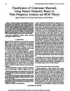
Fig. 5: Scatter plot of measured pixel intensity vs. distance to camera from the center pixel (i.e. u = 680, v = 512) in a set of 2180, 1360by-1024 pixel images. The scatter data exhibits an exponential falloff in intensity with distance from the camera due to attenuation, and a dependancy to colour.
where µy and σy2 are the desired mean and variance and µx (u, v, λ) and σx2 (u, v, λ) are the mean and variance of all intensities in a given set of N images at the pixel location [u, v] for a given channel λ. This process benefits from a large collection of N images within a given environment from different perspectives in order to provide a statistically significant measurement of µx (u, v, λ) and σx2 (u, v, λ) over objects of various colours and intensities. E. Image Transformation Accounting for Attenuation In addition to image spatial effects, such as lighting pattern and vignetting, attenuation also serves to skew the distribution of intensities measured at a given pixel location over an image set based on the range to different objects measured in each image. For example, Figure 5 illustrates a scatter plot of the red, green and blue image intensities measured from the center pixel (i.e. u = 680, v = 512) in a set of 2180, 1360by-1024 pixel images vs. the computed range in the scene of this image pixel taken from various perspectives over an underwater environment. The distributions in pixel intensities exhibit considerable correlation to the range to objects with a exponentially decaying relationship to range, indicative of the image formation model described in Equation 7. As in the case for lighting pattern and vignetting, rangedependent attenuation can be accounted for by applying an image transformation that is a function of image channel, image pixel coordinate and range to the object. The complete image transformation is thus computed as: Iy (u, v, λ) = m(u, v, λ, d)Ix (u, v, λ) + n(u, v, λ, d) s m(u, v, λ, d)
=
n(u, v, λ, d)
=
σy2 2 σx (u, v, λ, d)
(18)
(19)
µy − m(u, v, λ, d)µx (u, v, λ, d) (20)
where µx (u, v, λ, d) and σx2 (u, v, λ, d) are the mean and variance of all intensities in a given set of N images at the pixel location [u, v] for a given depth d and for a given
channel λ. One potential method for computing µx (u, v, λ, d) and σx2 (u, v, λ, d) is to ‘bin’ measured pixel intensities into specified values of d (distance from the camera) and compute the mean and variance of each bin, requiring a large number of samples at each bin, resulting in certain ranges and pixels locations being under-sampled. Since the expected distribution of intensities across different depths is expected to follow the relationship of image formation derived in Equation 7, an alternative approach is taken. For each pixel location, a scatter plot of image intensity vs. range is created, one point for each of the N image in the underwater dataset. If µR is the expected mean reflectance of the surface, then the mean image intensity measured from pixel [u, v], channel λ and range d is: µx (u, v, λ, d) = a(u, v, λ)µR e−b(u,v,λ)d + c(u, v, λ)
(21)
where a(u, v, λ), b(u, v, λ) and c(u, v, λ) correspond to parameters for the considered pixel location and image channel. Let a∗ (u, v, λ) = a(u, v, λ)µR and the parameters a∗ (u, v, λ), b(u, v, λ) and c(u, v, λ) in Equation 21 can now be estimated by taking a non-linear least-squares fit of this function with the scatter data using a Levenberg-Marquardt optimisation [10]. An initial state estimate x = [a, b, c] = [1, 0, 0] was used and was found to provide stable convergence in all of the datasets examined. The mean intensity is then computed from the function µx (u, v, λ, d) = a∗ (u, v, λ)e−b(u,v,λ)d +c(u, v, λ) as a function of distance d. To compute σx2 (u, v, λ, d), the variance corresponding to pixel [u, v] and channel λ as a function of distance d, a similar 2 is the expected variance of reflectance approach is taken. If σR 2 of the surface, then σx (u, v, λ, d) is: σx2 (u, v, λ, d)
= E[(Iy (u, v, λ, d) − E[Iy (u, v, λ, d)])2 ] =
2 [a(u, v, λ)e−b(u,v,λ)d ]2 σR
(22)
2 can be comThe expected variance of surface reflection σR puted using the parameters estimated in Equation 21; for each sample of the scatter data, the expected reflectance can be computed by taking the inverse of Equation 21 and from the 2 resulting values of reflectance, the variance σR is calculated.
IV. E XPERIMENTAL S ETUP Data collected from an AUV deployed in two different types of underwater environments was used to test the image correction techniques described above. The first dataset was collected over an underwater boulder field populated by various species of sponge, algae and sea urchins. The data was collected by taking overlapping transects of a rectangular region approximately 25-by-20m and contained images collected at various altitudes as the vehicle moved over the rocky terrain. The second dataset was collected from a single line transect over an area with various types of benthic coverage including rocky reef platforms with various species of coral, kelp and sandy bottom. In both datasets, the underwater terrain is rugous and results in images being collected from a range of different perspectives and ranges from objects in the environment.
The underwater images were collected using a stereo camera setup with two 1360-by-1024 pixel cameras; the left camera was a colour-bayer camera and the right camera monochrome (only images from the left camera were used in the image correction process). The cameras are mounted below the AUV platform looking downwards so as as to capture images of the terrain as the vehicle passed over. Images were captured in a raw 12-bit format and later converted to three colour channels. The camera firmware used a linear sensor response function. The aperture and shutter exposure times were fixed for each data collection. Artificial lighting was provided by two strobes attached to the AUV that provide white light to the scene. Both datasets were processed using a structure-from-motion pipeline [6, 9], and the derived 3D structure used to create range images for each left camera image collected. Two sets of corrected images were obtained from the raw data for both datasets for comparison. The correction was applied firstly using Equation 15 which only accounted for image space effects such as vignetting/lighting pattern and colour balance (i.e. not accounting for distance-based attenuation compensation). A second set of corrected images was obtained using Equation 18 which accounted for the full image formation model described in Equation 7 including image space effects and distance-based attenuation. Raw images were typically too dark to view with the naked eye (see Figure 4 for an example) and thus were not displayed in the comparisons shown. The corrected images were assessed both qualitatively (by examining consistency in appearance) and quantitatively by measuring the inconsistency in overlapping images of common objects. For each planar region of the surface model, a list of images that covered this region was compiled. The structurefrom-motion estimated image poses were used via backprojection to compute the patch of each image corresponding to the given spatial region. As a measure of inconsistency, the variance in these image texture intensities at this planar region was computed and displayed spatially over the map for each region. When images were affected by depth-based attenuation, regions that were viewed from multiple perspectives (and thus multiple ranges) displayed widely different texture intensities (and thus high variance and inconsistency) whereas when attenuation was compensated for, images of a common region displayed lower variance in intensity. The spatial patterns seen in the variance (i.e. faint banding patterns) correspond to changes in the number of overlapping views of each point. Some of the sharp peaks in variance correspond to small registration errors in the structure-from-motion process. V. R ESULTS Figure 6 illustrates examples of the mean and variance curve fitting using image intensity samples taken from the center pixel (i.e. u = 680, v = 512) from the 2180 images in data set 1 (boulder field). For a given value of distance d, the mean and variance values provide an approximation of the distribution of image intensities captured from various objects at this distance from the camera and are used to derive image correction
Fig. 6: Scatter plot of measured pixel intensity vs. distance to camera and estimated mean and standard deviation curves for each red green and blue channel for the center pixel, taken from 2180 images in dataset 1 (boulder field). The mean and variance (shown at three standard deviations from the mean) curves provide an approximation of the distribution of pixel intensities at a given distance from the camera.
parameters. The use of a fitting approach to compute statistics allowed for a robust estimate at ranges where only a small amount of data is present (i.e. very close or far away from the camera). Figure 7 illustrates a comparison between corrected images using the correction methods described in Sections III-D and III-E. The left subfigure illustrates an image that has been corrected using Equation 15 where only the spatial effects and colour channel are considered in the correction (i.e. no distance-based attenuation model). Although the image now has colours that are balanced and does not exhibit spatial effects such as vignetting or lighting pattern, there is still significant distance-based attenuation where regions of the image far from the camera (i.e. bottom right of the image) appear darker and more blue/green than regions close to the camera (i.e. top left of the image). The image in the right subfigure has been corrected using Equation 18 where all the effects of the image position, colour channel and distancebased attenuation are considered in the correction. Both the colour intensity and contrast in the more distant regions of the
Fig. 7: Left, colour compensated image using standard (non depth-based) correction and right, colour compensated image with full water attenuation correction. Both the intensity and contrast in the more distant regions of the image have been increased to match the overall scene in the right subfigure, while objects less distant have been darkened.
Fig. 8: Left, 3D photo-textured scene using standard colour corrected textures and right, 3D photo-textured scene using full water attenuation colour corrected textures.
Fig. 9: First and second subfigures from the top: comparison of 3D photo-textured scenes using standard and full water attenuation colour corrected textures. Third and fourth subfigures: comparison of image texture standard deviation for the same corrected textures (colourbar units are normalised intensity). The attenuation-corrected textures display significantly reduced variance in the intensity of images at each part of the map, in particular areas corresponding to large perspective changes by the vehicle.
image have been increased to match the overall scene, while the less distant regions have been darkened, largely removing the effects of attenuation. Once images were corrected across an entire dataset, they were applied as photo-textures for the structure-from-motion derived 3D surface model. Figure 8 shows a comparison of the photo-textured terrain model of dataset 1 (boulder field) when using image textures that have been corrected via the methods described in Sections III-D and III-E. The left subfigure illustrates the model using textures taken from images corrected using Equation 15 (i.e. no distance-based attenuation model) and the right subfigure illustrates the model using textures corrected using Equation 18 (i.e. full model with attenuation correction). The left model exhibits considerable correlation between the intensity/colour of image textures and the average distance from which each part of the surface was imaged from, in particular a horizontal banding pattern that corresponds to overlapping swaths during image collection that occur at slightly different heights above the terrain. The distance and general spatial correlation has been essentially removed in the corrected-texture model to the right. Figure 9 illustrates a similar comparison between phototextured models from dataset 2 (reef) with the non-attenuation corrected model shown in the first subfigure (from the top) and the attenuation-corrected model shown in the second subfigure. Inconsistencies are visible in the first model during passage of sections of rocky reef that sit above the sandy bottom and appear bright and red in the images as the AUV changes its height above the terrain in order to clear the obstacle. The bottom two subfigures illustrate maps of the variance in overlapping images textures across the map for the two different correction schemes. The attenuation-corrected textures display significantly reduced variance in the intensity of images at each part of the map, in particular areas corresponding to large perspective changes by the vehicle. VI. C ONCLUSIONS AND F UTURE W ORK This paper has developed an automated approach for correcting colour inconsistency in underwater images collected from multiple perspectives during the construction of 3D structure-from-motion models. Our technique exploits the 3D structure of the scene generated using structure-from-motion and photogrammetry techniques accounting for distance-based attenuation, and improves the consistency of photo-textured 3D models. Results are presented using imagery collected in two different underwater environments and demonstrated both the qualitative and quantitative improvement of the imagery. Our approach relies on the assumption of a ‘grey-world’ (i.e. one in which colours in the environment are grey on average and not biased in hue) and further more that this distribution is spatially consistent (in particular, depth). Future work will consider extensions to our approach to account for environments where this assumption could potentially be violated such as when objects of a particularly strong colour are only present at a biased depth in the dataset. One potential approach to this issue is to consider robustified fitting approaches or
outlier rejection methods that allow for a select, ‘well-behaved’ subset of the data to be used during model fitting. Future work will also consider approaches for building consistency in image datasets collected over multiple collection times, for monitoring long-term changes to the environment. R EFERENCES [1] G. Buchsbaum. A Spatial Processor Model for Object Color Perception. Journal of Franklin Institute, 310(1):1–26, 1980. [2] R. Campos, R. Garcia, and T. Nicosevici. Surface reconstruction methods for the recovery of 3D models from underwater sites. In IEEE OCEANS Conference, 2011. [3] R. Eustice, O. Pizarro, and H. Singh. Visually Augmented Navigation for Autonomous Underwater Vehicles. IEEE Journal of Oceanic Engineering, 33(2):103–122, 2008. [4] M. D. Grossberg and S. K. Nayar. Modelling the Space of Camera Response Functions. IEEE Trans. on Pattern Analysis and Machine Intelligence, 26(10):1272–1282, 2004. [5] J. S. Jaffe. Computer Modeling and the Design of Optimal Underwater Imaging Systems. IEEE Journal of Oceanic Engineering, 15(2):101–111, 1990. [6] M. Johnson-Roberson, O. Pizarro, S.B. Williams, and I. Mahon. Generation and Visualization of Large-scale Three-dimensional Reconstructions from Underwater Robotic Surveys. Journal of Field Robotics, 27(1):21–51, 2010. [7] S.J. Kim and M. Pollefeys. Robust Radiometric Calibration and Vignetting Correction. IEEE Trans. on Pattern Analysis and Machine Intelligence, 30(4):562–576, 2008. [8] D.G. Lowe. Distinctive Image Features from Scale-Invariant Keypoints. International Journal of Computer Vision, 60(2): 91–110, 2004. [9] I. Mahon, S. Williams, O. Pizarro, and M. Johnson-Roberson. Efficient View-based SLAM using Visual Loop Closures. IEEE Transactions on Robotics, 24(5):1002–1014, 2008. [10] D. Marquardt. An Algorithm for Least-Squares Estimation of Nonlinear Parameters. SIAM Journal on Applied Mathematics, 11(2):431–441, 1963. [11] Y.Y. Schechner and N. Karpel. Clear Underwater Vision. In IEEE International Conference on Computer Vision and Pattern Recognition, 2004. [12] A. Sedlazeck, K. Koser, and R. Koch. 3D reconstruction based on underwater video from ROV Kiel 6000 considering underwater imaging conditions. In IEEE OCEANS Conference, 2009. [13] L. A. Torres-Mendez and G. Dudek. A Statistical LearningBased Method for Color Correction of Underwater Images. In Research on Computer Science Vol. 17, Advances in Artificial Intelligence Theory, 2005. [14] I. Vasilescu, C. Detweiler, and D. Rus. Color-Accurate Underwater Imaging using Perceptual Adaptive Illumination. In Robotics: Science and Systems, 2010. [15] A. Yamashita, M. Fujii, and T. Kaneko. Color Registration of Underwater Images for Underwater Sensing with Consideration of Light Attenuation. In IEEE International Conference on Robotics and Automation, 2007.