Combating I-O bottleneck using prefetching: model, algorithms and ramifications Akshat Verma∗
Sandeep Sen†
Abstract Multiple memory models have been proposed to capture the effects of memory hierarchy culminating in the I-O model of Aggarwal and Vitter [?]. More than a decade of architectural advancements have led to new features that are not captured in the I-O model - most notably the prefetching capability. We propose a relatively simple Prefetch model that incorporates data prefetching in the traditional I-O models and show how to design optimal algorithms that can attain close to peak memory bandwidth. Unlike (the inverse of) memory latency, the memory bandwidth is much closer to the processing speed, thereby, intelligent use of prefetching can considerably mitigate the I-O bottleneck. For some fundamental problems, our algorithms attain running times approaching that of the idealized Random Access Machines under reasonable assumptions. Our work also explains more precisely the significantly superior performance of the I-O efficient algorithms in systems that support prefetching compared to ones that do not.
1
Introduction
Algorithm analysis and design are based on models of computation that must achieve a balance between abstraction and fidelity. The incorporation of memory hierarchy issues in the traditional Random Access Machine (RAM) model took some time [?, ?, ?, ?, ?, ?], eventually culminating in the I-O model of Aggarwal and Vitter[?]. The I-O model derives its acceptance from its simplicity. It manages to redress the lack of distinction among the memory access times of the different tiers of memory in the RAM model and has been used extensively in the design of various external memory algorithms [?, ?, ?]. Further work in this direction led to the Cache model of Sen, Chatterjee and Dumir [?] that addresses the algorithm design issues under the constraints of limited associativity in memory hierarchy. These results show an inherent gap between complexities of several problems between the RAM and the I-O models.
1.1
Motivation
The I-O models report their results in terms of the number of I-Os thus making the implicit assumption that every I-O has a fixed cost. Dementiev and Sanders [?] present an efficient sorting algorithm in terms of the I-O time thus moving to to a more practical metric. However, all these models assume that the cost of I-O (in terms of time) is a fixed constant. A close look at memory access reveals that I-O cost can be broken into latency (time spent in seeking to the right location) and the transfer time (time spent in actual transfer of the block). Hence, there is a latency L to paid before the transfer of a block can be started. A large number of techniques (like increase in bus bandwidth, advances in semiconductor technology) have led us to a stage where primary memory bandwidth is approaching processor speed. Similarly, the disk transfer times have significantly improved over the years where packing density and disk rotation speeds have greatly increased. Techniques like using multiple disks in parallel have also been useful to ensure that I-O bandwidth approaches processor speed [?, ?, ?]. Unfortunately, for the both primary and secondary memory the access latencies have not reduced in tandem with increase in memory bandwidth and processor speed so the I-O bottleneck is dominated by the access latency. The traditional theoretical approach for speeding up memory access has been to minimize the number of IO’s to reduce the total (sum of) latency and its parallelization on multiple disk architectures. Pipelining and Prefetching support in contemporary architectures (including Pentium IV) [?, ?] present another possibility, namely, overlapping access latencies (For a survey on system-level prefetching support, refer to [?] and references therein). Similarly, read-ahead caches on disks prefetch data in advance to hide the latency component. Also, ∗ IBM
India Research Lab, IIT Delhi, New Delhi 110016, India. E-mail:
[email protected]. of Computer Science and Engineering, IIT Delhi, New Delhi 1100116, India. E-mail:
[email protected]. Part of the research done when the author was visiting University of Connecticut and supported by NSF Grant ITR-0326155 . † Department
1
disk scheduling algorithms like SCAN hide latency of queued requests while serving a block. Because of the huge difference in magnitude between latency and transfer times, the potential savings in I-O times are immense. To take an example, consider a scenario where we read 1, 000, 000 10KB blocks sequentially where each read has a latency of 10 ms and transfer time of 0.1 ms per block. In the traditional I-O model we would incur a latency for each read and the total I-O time would be approximately 3 hours, whereas, with prefetching the total time is less than 2 minutes because we incur the latency only for the first block read. On current systems with system-level prefetching [?], such sequential reads take significantly less time than predicted by the I-O model (Section 5). In our experiments, we found that reading 640, 000 blocks without prefetching took almost half hour whereas prefetching allowed the sequential reads to complete in less than 10 seconds for a modern Seagate Cheetah disk (Section 5). Moreover, many recently proposed disk scheduling algorithms strive to compensate for the lack of prefetching-awareness in algorithms by idle waiting at a head position or waiting to build large batches of requests before sending them to the disk controller [?, ?]. In [?], the controller waits for more contiguous requests to be issued after serving a request, thus introducing idling. If such requests are issued before time using prefetching, such idling is eliminated thus increasing disk efficiency directly. Hence, incorporating prefetching in the I-O model not only ensures that the I-O times predicted by the model are meaningful but may improve disk efficiency as well. Moreover, algorithms designed for single cost I-O models [?, ?, ?] may not translate to optimal algorithms in a 2-cost prefetch model, since they do not specify the relative order in which blocks are fetched. Hence, such algorithms need to find an ordering of I-Os that is prefetch efficient (formally defined in Section 4). More importantly, computing a prefetch-efficient order of blocks ahead of time for certain problems (e.g. merge sort) necessitates devising new techniques. The experimental study in Section 5 shows that algorithms optimal in traditional I-O models but prefetch-unaware may perform very badly as compared to prefetch-aware algorithms.
1.2
Sorting and Transpose Examples
A common problem where an optimal I-O model algorithm does not perform well is merge sort. Consider the standard M/B-way merge sort, where we initially create N/M sorted runs, each of size M . These sorted runs are then merged recursively, taking them M/B at a time. Aggarwal and Vitter [?] show that M/B-way merge sort is optimal in the number of I-Os. However, this algorithm is oblivious to any prefetching support and, as a result, does not prefetch any blocks for skewed accesses across the runs. Note that for any prefetch order that the prefetchers use, an adversary can create an access pattern such that any prefetched blocks are not used. As a result, it incurs latencies for most I-O requests. On the other hand, the much simpler 2-way merge sort is able to prefetch a large number of blocks if the prefetcher reserves half of memory for each of the 2 runs being merged. (A formal proof is described in the appendix.) Hence, it is able to hide latencies for most of the blocks and outperform the M/B-way merge sort, which is a superior algorithm in the traditional I-O model. Hence, it becomes imperative to enhance the I-O model to take prefetching into account in order to design better algorithms. Moreover, the I-O time of algorithms that use prefetching, either ordinately or inordinately, as predicted by I-O model, is much more than their actual I-O times. This is because each I-O request has to incur a latency in the I-O model, whereas such latencies may be hidden by the prefetching support available. In order to validate this observation, we conducted two experiments with M/B-way matrix transpose, first with prefetching disabled and then with prefetching enabled. We found that with prefetching enabled, the total time is reduced by a factor close to 300 for the disk model used. (A detailed experimental study and setup is described in Sec. 5.) Hence, in order for the running times predicted by the I-O model to be meaningful, such prefetching support needs to be incorporated in the model.
1.3
Results
We propose a formal prefetch model based on traditional I-O models that incorporates prefetching support available. We make some insightful observations on the similarities between the prefetch model and Parallel Disk Models (PDM) and use them to design an emulation scheme to convert optimal PDM algorithms to algorithms optimal in prefetch model. We also present techniques to design algorithms directly for the prefetch model for the cases where either such PDM algorithms do not exist or are not very practical on real systems. We present the novel techniques of sequence preservation for straight-line algorithms, dynamic rebalancing of prefetched data for merging constant number of sequences and prediction sequence balancing for merging large number of sequences. The techniques provide optimal algorithms for many common problems like Matrix Transpose, Sorting, Permuting and FFT. We also extend the prefetch model to incorporate (a) parallel disks, (b) limited prefetch buffers,
2
(c) small associativity and (d)limited streams support for prefetching. Finally, we present an experimental study to demonstrate that incorporation of prefetching in the memory model allows us to make better estimates of I-O time and use algorithms that perform better on current systems.
1.4
Prefetch and Related Models
In order to take advantage of prefetching, we work with a two-level memory model where the I-O cost is in terms of two parameters - L is the time to access the memory location and BM is the transfer time for a memory block of size B. The request for accessing a block from the slower memory can be sent out prior to its actual use and moreover several such requests can be pipelined. This model has some similarities to [?] where L = f (xℓ ) is a (monotonic) function of the last address xℓ in a block transfer and additional cost 1 thereafter. The authors had derived bounds for different families of the function f . By choosing a step function L (left open by [?]), in conjunction with other parameters of the I-O model our algorithms exploit features hitherto not analyzed. We would like to note that some of the recent experimental studies of external sorting [?] make extensive use of parallel threads which may invoke prefetching at a system level. In another approach the authors [?] look at oblivious sorting algorithms on a multi-disk machine where prefetching could turn out to be extremely relevant. An orthogonal field of study that has attracted a great deal of attention is the design of efficient system-level prefetching techniques independent of the algorithm running on the system [?, ?]. The focus of such techniques has been to identify regular data access patterns amongst the I-O requests and prefetch data accordingly. However, if the algorithms running on such systems are unaware of prefetching, the system-level prefetchers may not be effectively used. Hence, we design algorithms that efficiently use such prefetching support to reduce I-O times.
2
The Prefetch Model and some Preliminaries
Aggarwal and Vitter [?] proposed an I-O model for an input of size N that reads blocks of size B, can transfer D blocks concurrently and works with a fast memory of size M . For completeness, we summarize their results in the appendix. We formalize an extension of the I-O models that allows algorithms to use prefetching in architectures that support it. We use M and B to denote the size of fast memory and the block size respectively. In addition, we introduce the following additional parameters • BM as the time1 to transfer one block of memory, where BM /B ≥ 1. • L as the normalized latency in transferring from slow memory to fast memory. We always use L to denote read latency unless otherwise stated. In cases where we deal with both read and write latency, we use Lr to denote read latency and Lw to denote write latency. • There is an explicit prefetch instruction and the Prefetch Latency is also L. In current systems, we can prefetch blocks only as part of some stream access. The above assumption is used only for the lower bound proofs and the blocks prefetched by our algorithms are always stream accesses. To simplify our presentation, we initially remove the parameter D from the prefetch model and propose optimal algorithms in a single disk prefetch model. We then propose techniques to enhance the algorithms to work in a parallel disk scenario. We show that every single disk algorithm has an enhanced version using one of the techniques that is optimal in the parallel disk prefetch model. Our parallel disk model differs from [?] since we have the restriction that the D I-Os performed in parallel should access D distinct disks. In this paper we make the following assumptions that are consistent with the existing architectures. (i) N > M > B (ii) (M/B)BM > L (iii) N, M, B are of the form 2i to simplify analysis - the asymptotic bounds are not affected. The fast memory size (be it cache or registers) M is typically much larger than the size of the cache line B. Moreover, the latency incurred, L, is typically much smaller than the time to load the internal memory completely (= M B BM ). Prefetch latency is typically same as the memory latency L or may differ from it by one or two cycles. Definition 1. The latency li of block i is defined as the additional latency that is incurred because of block i. Hence, if reads for block (i − 1, i) are given at (ti−1 , ti ) and the blocks are available at times (ei−1 , ei ), then li = ei − max{ti , ei−1 }, where ei ’s are sorted. Note that if reads are blocking, then this definition of latency is the same as li = ei − ti , which is the one commonly used. We modify the usual definition in order to define cumulative latency of a m − block Lm simply as sum of the latency of the m blocks, where an m − block denotes a set of m consecutive blocks. fi denotes the ith block of fast memory and sj the jth block of slow memory. We would like to make a note here that complete 1 All
the timing parameters are normalized wrt to the instruction cycle
3
control over prefetch is not realistic and, in practice, prefetching is constrained by the number of prefetch buffers, limitations due to associativity (in a Cache Model) and some kind of streaming behavior in data access required for most forms of prefetching. We address the architectural constraints later and note that all our algorithms exhibit streaming behavior that is required for prefetching in current architectures. Running time We analyze the algorithms in terms of the total time that includes computation time and the I-O time. This is normalized with respect to the instruction cycle that takes unit time. The only I-Os (reads/writes) that we consider are I-Os to slow memory. Access to fast memory is counted along with the number of I-O operations. Since, the memory bandwidth is now within a small constant factor (2 to 4) of the processor speed, the running times that we derive have a multiplicative factor of BM /B, which is O(1) when BM = cB for some constant c.
2.1
Lower Bounds in the Prefetch Model
In the prefetch model, a block that has not been prefetched takes time BM + L, whereas a block that has been prefetched takes BM time. It is easy to see that if k is the minimum number of I-Os needed to solve a problem A, then kBM + L is the lower bound on total time in the prefetch model. The bound is obtained by assuming that there exists a prefetch algorithm that prefetches all but the first block. Similarly, if there exists an algorithm that uses k I-Os, then k(L + BM ) is the upper bound on the I-O time by multiplying the number of I-O’s by the time to transfer each block without prefetching. This upper bound is same as the lower bound on I-O time in the traditional I-O models. This general lower bound and (M/B)BM > L combined with the bound on the number of I-Os for individual problems [?] yields the following bounds in our prefetch model. For D disks, the lower-bounds are divided by D. Theorem 1. The worst case I-O time required to sort N records and to compute any N-input FFT digraph or an N-input permutation network is N log(1 + N/B) BM ) (1) Ω( log(1 + M/B) B Theorem 2. The worst case I-O time required to permute N records is Ω(min{N BM ,
N log(1 + N/B) BM }) log(1 + M/B) B
(2)
Theorem 3. The worst case I-O time required to transpose a matrix with p rows and q columns, stored in row major order under the assumption that M > B 2 , is Ω(N BBM ).
3
Prefetch Model and PDM Algorithms
We now investigate similarities between algorithms in a Parallel Disk Model (with D = M/B) and algorithms in the proposed Prefetch Model. We observe that both class of algorithms need to exploit essentially the same features in memory access. One may note that if a prefetch model algorithm can perform M/B I-Os in a pipelined fashion and hide the latency of all but the first of these M/B blocks, it would be efficient, i.e., it would take O(BM ) time to perform a block I-O (since L < (M/B)BM )). Similarly, a PDM algorithm with M = DB needs to perform M/B I-Os concurrently and hence needs to predict the next M/B blocks needed next. Moreover, in both these models, if the algorithm performs the minimal number of I-Os possible while maintaining the M/B order pipelining or parallelism respectively, the algorithm is optimal in the respective model. This general idea has also been proposed in [?] to design efficient serial algorithms from parallel versions. We now present an emulation scheme to generate Prefetch Model algorithms from P DM algorithms using this insight.
3.1
PDM Emulation
We restrict P DM algorithms to only those parallel disk algorithms that deal with the case M = DB. The emulation works in the following manner. The sequential algorithm with prefetching performs I-O in blocks of D. It emulates the D disks as contiguous locations in D zones of the single disk. For every parallel I-O pi performed by the PDM algorithm, let Si be the set of D I-Os that the PDM algorithm performs concurrently. The emulation algorithm starts the prefetch of all these |Si | blocks together. When all the |Si | blocks are available in the fast memory, the emulation algorithm starts prefetch of the blocks in Si+1 corresponding to the next parallel I-O pi+1 . We show the following result Theorem 4. If the PDM algorithm performs k parallel I-Os, the corresponding sequential prefetching algorithm takes an I-O time of O(kDBM ).
4
Proof: The proof is immediate by estimating the I-O time corresponding to each parallel I-O. Each batch of Si block I-Os takes an I-O time of L + DBM . Since D = M/B and (M/B)BM > L, the I-O time for the block I-Os corresponding to each parallel I-O is only O(DBM ). Multiplying it by the number of parallel I-Os k leads to the desired result. A similar emulation scheme is obtained for parallel disk prefetch algorithms with the number of parallel disks D′ < D. In a parallel disk prefetch model, we make the additional assumption that the fast memory available per disk is large enough to hide the latency for that disk, i.e., DM′ B BM > L. Each of the D′ disks now emulate D/D′ disks and we have the following result. Theorem 5. If the PDM algorithm performs k parallel I-Os, the corresponding parallel prefetching algorithm with D′ disks takes an I-O time of O(kD/D′ BM ). The above emulation scheme allows us to convert existing optimal PDM algorithms to algorithm optimal in our prefetch (sequential or parallel disk) model. It is easy to see that if a PDM algorithm is optimal in the number of parallel as well as block I-Os (i.e., it performs the minimal number of parallel I-Os as well as the total number of block I-Os across all the disks is minimum), the corresponding emulated prefetch algorithm is optimal in the prefetch model. Since the lower bound for most common problems in a PDM model is a factor D′ (number of disks used) less than the lower bound in a sequential I-O model, an optimal PDM algorithm is also typically optimal in the traditional single disk I-O model. Hence, in most likelihood, such optimal PDM algorithms can be directly used to generate an optimal prefetch algorithm.
3.2
Drawbacks of PDM Emulation
We have presented an emulation scheme for converting optimal PDM algorithms to optimal algorithms in the prefetch model. However, designing optimal PDM algorithms has proven to be quite difficult and a large number of algorithms designed for PDM model are quite complicated. As we shall see, simpler algorithms can be designed for many problems by direct design. Moreover, there are practical constraints on the PDM algorithms imposed by current architectures that support prefetching only for streamed accesses. Hence, the access pattern for the algorithm (PDM or otherwise) for each disk should be regular and streamed. The PDM algorithm should also ensure that other practical constraints (e.g., limited prefetch buffers, associativity) are not violated. As we will see later, the constraint of streamed access is not always satisfied by P DM algorithms. Since the P DM model cannot be naturally extended to capture such practical constraints, P DM algorithms may need to be modified to work well in the prefetch model. A big disadvantage of emulating a PDM algorithm in the prefetch model is that the PDM algorithm may not allow overlap of I-O and computation. The basic reason for this difficulty lies in the fact that the emulation strategy tries to fill a complete memoryload (M records) together, since it emulates a parallel read/write of M/B blocks. On the other hand, algorithms obtained by direct design predict the next required block only and fetch it while computations are performed on earlier blocks. This allows them to use most of the blocks in memory for computation allowing them naturally to overlap I-O and computation. Hence, we present new techniques to design algorithms in the prefetch model next and show that these general techniques can be employed to design fairly simple algorithms for a large class of problems.
4
Designing Optimal Algorithms Directly
The different techniques (from prediction sequence balancing to sequence preservation) employed for direct design of algorithms have a common underlying strategy: perform minimal number of I-Os in a prefetch-efficient manner, i.e., hide latency for all blocks other than the first. Definition 2. An algorithm that performs k I-Os is prefetch efficient if it takes I-O time O(L + kBM ). We have essentially devised three techniques for designing optimal algorithms. We prove a general result for a class of algorithms called sequence-preserving algorithms and use it to design optimal algorithms for all straightline algorithms considered (e.g., matrix transpose, permutation and FFT). We have devised a technique for dynamic rebalancing of prefetched data for algorithms that merge constant number of sequences (2-way sorts) and prediction sequence balancing for algorithms that merge large number of sequences (M/B-way sorts). We first present results for sequence-preserving algorithms and show some applications of the result.
4.1
Sequence Preserving Algorithms
We start with stating the following result that is easy to obtain. Lemma 1. For any set of k pre-determined block reads, the total time needed is O(L + kBM ). 5
A(1) 0
BM 2BM
L
A(k) L+BM (k−1)B M
L+(k−1)B M L + kBM
P(k)
P(1)
Time Line
P(i) = Prefetch for block i is given A(i) = First element of block i is available. Figure 1: Timing Diagram for Prefetch Schedule S Proof: Note that since the reads are pre-determined, the prefetch instruction for any block can be given at any time. Hence, a simple schedule S (Figure 1) that prefetches blocks in the same order as they need to be read and interleaves consecutive prefetches by BM units of time would read all the k blocks in L + kBM time. In fact, the schedule prefetches the ith block in L + iBM time, ∀i ≤ k. We now define a class of straight-line algorithms that we call sequence-preserving algorithms and prove that in this class of algorithms, prefetching can hide latency. We will later show that many straight-line algorithms fall in this class. We begin with some definitions. Definition 3. An instruction Ii precedes Ij in an algorithm A (i.e. Ii < Ij ), iff Ii is executed before Ij in A. We also define I w,i and I r,i as the sets consisting of all the instructions that write and read respectively from memory location si . We order the instructions in the set in the order of their usage in A. Definition 4. The neighbourhood set NI is defined as a set containing all the tuples of the form {I1 , I2 } such that I1 , I2 ∈ {I w,i ∪ I r,i , I w,j ∪ I r,j } for some i, j and there does not exist I3 : I3 ∈ (I w,i ∪ I r,i ∪ I r,j ∪ I w,j ) and I1 < I3 < I2 or I2 < I3 < I1 . The neighbourhood set of an algorithm A consists of tuples {I1 , I2 } of instructions such that I1 and I2 access (read or write) memory locations si and sj at times T1 and T2 respectively. Also, none of the instructions in A executed between T1 and T2 access either of the two memory locations. We also define for all instructions of ∗ the form Im ∈ I w,j , ∗ Im as the last instruction in I r,j s.t. ∗ Im < Im and Im as the first instruction in I r,j s.t. ∗ Im < Im . Definition 5. A straight-line algorithm A is sequence preserving iff for all I1 and I1∗ , s.t. (i) ∃{∗ I2 , I1 } ∈ NI or ∃{∗ I2 ,∗ I1 } ∈ NI and (ii) ∗ I2 < I1 ; then, (a)I2 exists,
(b){I1 , I2 } ∈ NI (c) I1 < I2 ⇔ I1∗ < I2∗ .
(3)
Essentially, a sequence preserving algorithm reads data in the same order as it had last written them, if it had written them earlier. Moreover, before reading any data that had been written earlier, all the reads before that write should also be written back. For the cases where any of the {I1∗ , I2∗ } or {I1 , I2 } are not defined, the corresponding precedence relation in Equation 3 is assumed to hold by default. Using the following lemma, we show (proofs in Appendix) how to convert existing I-O optimal sequencepreserving algorithms to prefetch-efficient algorithms. Lemma 2. For any I-O optimal sequence-preserving straight-line algorithm A, there exists a sequence-preserving algorithm A′ such that if a write of block si of slow memory is made at time t, the read to block si of slow memory is made after at least M/B block I-Os. Also, A′ performs no more I-Os than A and hence is also I-O optimal. Proof: The proof is by constructing an algorithm A′ from another algorithm A that does not satisfy the required property. Assume that in A, a write (I1 ) is made from fh to si at time Tw and a read (I1∗ ) from si to block fl is needed at time Tr = Tw + jBM . We denote Tp as time of the read from si prior to I1 . Also, assume that j < M/B. We now categorize all the reads that took place before Tw . We only consider the last reads from any location.
6
Let j1 be the number of reads that have been written back between Tp and Tw . Let ∗ I0 be any such read. Then I0 < I1 , {∗ I1 ,∗ I0 } ∈ NI and I0 < I1 . Hence, by Eqn.3, I0∗ < I1∗ , i.e., the block would be read again before the next read of si (= Tr ). Thus, there would be j1 such reads between Tw and Tr , one for each of the j1 writes. Let j2 be the number of reads that had not been written back between Tp and Tw . For every such read ∗ I2 , either {∗ I2 , I1 } ∈ NI or {∗ I2 ,∗ I1 } ∈ NI . Also, since ∗ I2 < I1 , we have {I1 , I2 } ∈ NI . Therefore the corresponding write I2 would be done before Tr . Hence, the total number of such writes are at least j2 . If there are j3 other reads between Tw and Tr , then the total number of memory locations used are bounded by j1 + j2 + j3 . Also, j1 + j2 + j3 ≤ j < M/B and as a consequence, we have at least 1 block fm of fast memory free that can be used to avoid the write I1 . We can simply replace the write I1 and read I1∗ in A by two move instructions that moves the block from fh to fm and fm to fl respectively to get A′ . We can do this one by one for all such write-read combinations to get A′ for which no such write-read combination exists.
∗
Note that even the move instructions are not required. Instead, the code could be changed to swap usages of fh and fm until fh and fm are written back to slow memory. Also, even though we denote Tp as the time for previous read, the proof is valid even if a write to si is not preceded by a read from si . We can simply assume that the read took place just before the write, i.e. Tp = Tw , and the proof carries through without any change. One may also note that an I-O optimal algorithm in general may not be the optimal algorithm for that problem. However, we show that the I-O optimal algorithm does not take computation time more than the I-O time and hence, it is also optimal. Theorem 6. Any sequence-preserving straight-line algorithm that uses k I-Os has an equivalent algorithm that takes I-O time O(L + kBM ). Proof: Note that in the case of any straight-line algorithm A, the sequence of reads is known a priori and Lemma 1 holds. However, if a read is preceded by a write of the same block, then the prefetch can not be started arbitrarily early. In fact, the read can only be started after the write has been completed. However, by Lemma 2, there exists an equivalent algorithm A′ such that the write and read to any block are separated by at least M/B I-Os. If the original algorithm A does not satisfy this property, then the equivalent algorithm A′ can be constructed using the proof of Lemma 2 and used. We now look at the first of M/B blocks such that the block si is to be written at Tw and read at the earliest possible Tr = Tw + jBM , where by Lemma 2 j equals M/B. Also, the time that is needed for a write to block si followed by the corresponding read is Lr + Lw . Note that the minimum number of blocks that would be written and read in the above time is at least j = M/B. Including the read of the block si , we have M/B + 1 reads. Hence, the average time to read a block, other than the first (M/B+1) Lr +Lw block, is bounded by max{ BM (M/B+1) , (M/B+1) }. Assuming Lw = BM (time to write back a block), which is true for write back, and using the fact that Lr (= L) < M BM /B, we get a worst case bound of BM . Assuming Lw = Lr , we get a bound of 2BM , which again gives us the bound of O(L + kBM ) for the k I-Os. Corollary 1. A sequence of k pre-determined reads, k ≥ M/B, takes time O(kBM ). Corollary 2. A sequence of k pre-determined reads and writes, k ≥ M/B, such that no writes follow reads, i.e., there does not exist a pair I1 , I2 ∈ {I w,i , I r,i }s.t.I1 < I2 for some i, takes time O(kBM ). The proofs of the corollaries follow directly from the above theorem and the fact that L < (M/B)BM . We have now characterized a class of algorithms such that prefetching is able to hide the latency in reading the blocks. We now specify a writing order for various I-O optimal algorithms and use Theorem 6 to devise algorithms optimal in the prefetch model. 4.1.1 Matrix Transpose Algorithm: We show that the following transposition-by-blocks algorithm is sequence-preserving. The algorithm transposes sub-matrices with B rows and B columns. It transposes the B rows by taking M/B rows at a time and computing the partial transposes. While writing them back, the algorithm ensures that it writes them in the order they need to be read. It then iterates till the transposition is complete. After computing all the block transposes, it rearranges the blocks in the required order taking linear time. Our writing order immediately ensures that our algorithm is sequence-preserving. If M/B > B, then the algorithm needs only one pass of the data to compute the block transposes. This leads to the following corollary of Theorem 6.
7
Corollary 3. The total time to transpose a matrix with p rows and q columns, stored in row major order, is Θ(
BM N) B
(4)
Note that even in the case that M < B 2 , the above algorithm is sequence preserving. Moreover, the number of I-Os required in that case matches the lower bound of Aggarwal and Vitter for the general case (Lemma 13). Hence, the algorithm runs in time equal to the lower bound for the problem. 4.1.2 General Permuting Algorithm: Note that permuting is a special case of sorting. The algorithm for permuting is thus based on the M/B-way merge-sort algorithm of [?]. The algorithm has two phases. In the first phase, we permute the elements within runs of size M . Later, we merge the permuted runs taking them M/B at a time. The difference from merge sort though is that the the next set of blocks needed is known a priori in this case. We have the following theorem for permuting. Theorem 7. The total time required to permute N records is Θ(min{N BM ,
N log(1 + N/B) BM }) log(1 + M/B) B
(5)
Proof: The key idea of the proof lies in the observation that the next set of blocks needed in fast memory are known a priori in case of permutation whereas, it is not known in the case of sorting. Hence, Lemma 1 is applicable for the permutation version of merge-sort. Also, Corollary 2 can be directly applied to each pass of the data because (a) the length of each of the N/M runs is larger than M and (b) each run is read only once in each pass. This in conjunction with the bound on the number of I-Os for sorting (Lemma 11) yields the bound log(1+N/B) BM of O( Nlog(1+M/B) B ). The first part of the minimizing expression is obtained by the naive algorithm that reads one element at a time and writes it to its proper location. Hence, N reads and writes are needed. Moreover, the sequence of reads and writes are known and Corollary 2 yields the bound of O(N BM ). 4.1.3 BMMC Permutations General Permutation has an I-O time that is bounded by the number of I-Os needed for sorting. However, for a large class of permutations, the I-O time can be significantly reduced. Cormen et al. [?] propose algorithms for a class of bit-matrix-multiply/complement (BMMC) permutations and show that they perform optimal number of I-Os in a parallel disk model. We have shown that the algorithm is sequence-preserving and hence, its I-O order obtained by Theorem 6 is optimal. A BMMC permutation is specified by an log N × log N characteristic matrix Λ = (aij ) whose entries are drawn from {0, 1} and is non-singular (i.e. invertible) over GF (2) (operations modulo 2). The specification also includes a complement vector c of length log N . A target address vector y is derived from a source address vector x as y = Λx ⊕ c. Cormen et al. [?] factorize the characteristic matrix Λ into a set of matrices, each of which is either a Memoryrearrangement/complement (MRC) or memoryload-dispersal (MLD) permutation. They show that any MRC or MLD permutation requires only one pass of data. If we partition the N records into N/M consecutive sets, each of size M , each set is called a memoryload. Hence, memoryloads are numbered from 1 to N/M . Each MRC permutation can be performed by reading in a memoryload, permuting its records and writing it out to same or another memoryload number. Since for each MRC, no writes follow reads, it is sequence-preserving. Similarly, a MLD permutation reads a memoryload and writes it in a balanced fashion over all the parallel disks (a single disk in the sequential case) and is also sequence preserving. Hence, a combination of MRC and MLD permutations is also prefetch-efficient. Since the algorithm in [?] is based on factorization of a BMMC permutation into a sequence of MRC and MLD permutations, it is also prefetch-efficient. Moreover, since it is also optimal in the number of I-Os, it is optimal in our prefetch model. For further details on the factorization of BMMC or the proof that MRC and MLD permutations can be performed in one pass, refer to [?]. 4.1.4 FFT and Permutation Networks We show that the algorithm for FFT and Permutation network proposed in [?] is sequence-preserving. Hence, an I-O order obtained using Theorem 6 is prefetch-efficient and we have the following optimality result. It is well known that three FFT networks concatenated together form a permutation network. Hence, we consider 8
algorithms only for FFT digraph. We show that the algorithm for FFT network proposed in [?] satisfies the lower bound of Theorem 1. FFT algorithm: The FFT digraph is decomposed into (log N )/ log M stages, where stage i, for 1 ≤ i ≤ (log N )/ log M , corresponds to the computation of columns (i − 1) log M + 1, (i − 1) log M + 2, ...., i log M in the FFT digraph. The M nodes in columns (i−1) log M that share common ancestors in column i log M are processed together in a phase. In order to do that, the N records are permuted by a transposition permutation in a manner such that the M records required in a phase can be brought together. Note that after the transposition, data access for each stage is just one pass through the data. This is followed by computation of the next log M columns in a similar manner. Transposition Permutation: The transposition are done in a manner that also covers the simple matrix transpose. A target subgroup of a group of records is defined as a subset of records that remain together in the final output. The records in the same target subgroup remain together throughout the course of the algorithm. In each pass of the input, target subgroups are merged M/B-way and hence, the size of each subgroup is increased by a multiplicative factor of M/B. This is repeated until the transposition is complete. For further details of the passes of data are algorithm, please refer to [?]. A straightforward analysis would then show that log min{M,N/B} log M/B required for each stage. Also, since no block is read twice, no reads follow the writes in a pass. Hence, corollary 2 holds for each pass. Therefore, each pass would need time no more than O(N BM /B). This gives us a bound of O((N
BM log min{M, N/B} log N ) ) B log(M/B) log M
(6)
A simple analysis of the two cases {M > N/B, M < N/B} then leads us to the following theorem. Theorem 8. The total time required for computing a permutation network is Θ(
4.2
N log(1 + N/B) BM ) log(1 + M/B) B
(7)
Dynamic Rebalancing: Merge Sort
We illustrate the technique of dynamic rebalancing of prefetched data (balancing the amount of data being prefetched across all runs) using 2-way merge sort and show that it matches the I-O time to the Compute Time, i.e., O(N log N ). Merge Sort Algorithm: The merge sort algorithm is identical to the standard 2-way merge sort. Our prefetching strategy is the one that achieves the bounds needed. We describe our prefetching algorithm for the merging procedure of merge-sort first. We define A1 and A2 with sizes n1 and n2 as the two sorted arrays that are to be merged. Without loss of generality, we assume that n1 = n2 . Case (i) : n1 > M/2. The prefetch algorithm prefetches M/(2B) blocks of both the arrays and labels them from 1 to M/(2B). It then prefetches the next block from A1 if the last element of block 1 of A1 is smaller than the last element of block 1 of A2 . Otherwise, it prefetches the next block of A2 . If it prefetches from A1 , then it decrements the label on each block of A1 by 1. Otherwise, it does the same for A2 . The prefetching evaluation is performed every BM cycles and either of A1 or A2 is prefetched depending on the evaluation. If at any time there are no blocks of A1 left to be prefetched, the next block to be prefetched is from A2 and vice versa. If both A1 and A2 have no blocks left to be prefetched, case (ii) is followed. Case (ii) : n1 ≤ M/2. The prefetch algorithm prefetches (M/2B) blocks each from both the arrays and labels them from 1 to M/2. It then starts prefetching the next set of arrays as the blocks of A1 or A2 are written out to slow memory, i.e., at most once every BM cycles. Note that the data manipulation in merge-sort is done only in the merging procedure. Hence, the reads are done just prior to merging. The merge-sort is performed in this manner. We initially load M/B blocks of the array and merge-sort them. We do this for all the (N/M ) M/B − blocks. Hence, after this step, we have (N/M ) M/B − blocks that are all sorted and have to be merged taking them 2 at a time, with the size doubling in each iteration of merge-sort. The prefetching algorithm for merging described earlier is then used for the remaining iterations. 9
The prefetching procedure allows us to make one prefetch every BM cycles. We will show later that the I-O time in the first log M iterations of merge-sort is less than compute time and hence prefetching is not needed in some BM cycles. This leads us to the following claim. Claim 1. If the prefetch of block si is made at time Ti , it is available in fast memory at time Ti + L, i.e., there would never be any pending prefetch. For the sake of analysis, we divide the run of merge-sort algorithm into two phases. Recall that merge-sort needs O(log2 N ) recursive iterations where in each iteration the size of the arrays to be merged increases from 1 to N . The first phase is then a combination of the first log2 M iterations. The second phase comprises of the rest of the iterations. The following results hold for the two phases (proof in Appendix). Lemma 3. The total I-O time in the first phase of merge-sort is O(N BBM ). Proof: In the first phase, we need to read any block from slow memory si only once. We load the required M/B blocks into fast memory, sort them and then write them out to slow memory. As a result, we incur a latency N/B , i.e., N/M . Hence the total of L for every M/B − block. Note that the total number of M/B − blocks are M/B LN latency incurred is M . As we have (M/B)BM > L and BM > B, the total latency is bounded by N . Hence, the total I-O time required is N + N BM /B, which is O(N BM /B). Lemma 4. The total I-O time of the second phase of merge-sort is at most (2N
N BM ) log2 +L B M
(8)
N Proof: Note that we have a total of log2 M iterations of merge-sort left. We show that each iteration, other than the first, takes time no more than 2N BM /B and the first iteration takes time 2N BM /B + L. We prove the following lemma first that relates the latency incurred in reading a block si with the latency incurred by its neighboring blocks.
Lemma 5. The cumulative latency for any k − block, k ≤ BM block of A1 and A2 is bounded by max(L − M 2 B , 0).
M 2B ,
that is disjoint from the first M/(2B) −
M/B Proof: We only prove the case L > M/B 2 BM and note that if L < 2 BM then it can be shown that the latency is 0 using a reasoning similar to Theorem 6. The exception part of the lemma is to account for the fact that the initial M/(2B) − block of the first A1 and A2 are fetched deterministically and not in the same manner as the remaining blocks. We will analyze the I-O time for those blocks separately. The proof of the lemma is by induction on k. Base Case: k = 1. Let T0 be the time at which the prefetch for the block si is started. The read M request for si would be made no earlier than T0 + MB 2B , as there are M/2 numbers to be read before reading si . Also, note that si would be available at T0 + L. Hence, the total latency is at most MBM M (T0 + L) − (T0 + MB 2B ) = L − 2B . Let us assume now that the hypothesis holds for m blocks 1 ≤ m < M/(2B), i.e., the cumulative latency M Lm ≤ L − MB 2B . We now look at the time Tm+1 at which the prefetch instruction for the (m + 1)th block sm+1 was given. Note that sm+1 would be available at time Tm+1 + L. Also, note that the read to sm+1 would be made th M block at time later than Tm+1 + Lm + MB 2B . Hence, the latency for the (m + 1)
lm+1 i.e., lm+1 i.e., lm+1 + Lm i.e., Lm+1
≤ Tm+1 + L − (Tm+1 + Lm + M ≤ L − Lm − MB 2B MBM ≤ L − 2B M ≤ L − MB 2B
MBM 2B
)
MBM M The above lemma leads to the fact that the total time for reading a M/(2B)− block is at most (L − MB 2B )+ 2B , which is bounded by M BM /B. Also note that prefetching of consecutive merges are also pipelined in this procedure. Hence, the total time required for 2N M blocks is 2N BM /B. Recall also that the procedure pipelines merges
10
N N iterations would take time 2N BM /B log2 M . However, from consecutive iterations as well and hence the log2 M since the two phases are not pipelined, the first M/B − block of the first A1 and A2 would suffer latency of MBM M instead of L instead of L − MB 2B . The total time to be accounted for these blocks would then be L + 2 2B 2M BM /B and hence the additional latency between the two phases would be L. Hence, we get the bound of N + L for the second phase. 2N (BM /B) log2 M End of Lemma 4
Since we have not changed the merge-sort algorithm, the number of comparisons in merge-sort remain O(N log N ). N + L. Also, the I-O time is the sum of the I-O time of both the phases, i.e., O(N BM /B) + 2N (BM /B) log2 M BM N Since the second phase is required only if N ≥ 2M , we have the I-O time bound of O(N B log M ). Hence, the total time is bounded by O( BBM N log N ). Thus, we have the following theorem. Theorem 9. The total time required to sort N numbers using 2-way merge sort in the prefetch model is O( BBM · N log N ).
4.3
Randomized Merge Sort with Prediction Sequence Balancing
Although the two way mergesort has Θ(N log N ) running time, it does performs more passes than an I-O optimal algorithm. It is easy to verify that the standard M/B-way Merge Sort [?] is unable to hide the latency for most blocks because an adversary may force it to prefetch blocks out of order of their use. Since it has only constant memory available per run (as opposed to 2-way Merge Sort that had M/2 memory available), it can hide latency only for a constant fraction of blocks. The strategy of using a prediction sequence [?] used for parallel disks works either for small N (N/B < M ) or requires the complication of forming large meta-blocks a priori, which additionally increases the constants. Similarly, Columnsort algorithm [?] uses some novel techniques to ensure that data access is deterministic but makes the assumption that N < (M/p)3/2 . Hence, even though it can be shown to be prefetch-efficient, the algorithm is not defined for large N . We also pursue the idea that if an algorithm A could predict the order in which blocks are needed in any merge phase of the merge sort algorithm, A would be prefetch efficient, i.e., A would take O(kBM ) time to perform k I-Os. We use the simple idea that an O(M ) sample of prediction sequence is sufficient for predicting, with high probability, the order in which blocks are needed, if the prediction sequence is balanced across all the runs being merged and the input is randomized. Hence, the technique is in some sense, a refinement of balancing prefetched data, the difference being that instead of balancing data over runs (as in Sec. 4.2), we now balance the prediction sequence across runs. Note that if we prefetch blocks in exactly the order that they are needed in memory, the I-O time for reading k blocks would be kBM + L, i.e., the algorithm would be prefetch efficient. We describe the optimal M/B-way merge sort (optimalSort) algorithm in Fig. 2. Algorithm optimalSort Randomize the input Divide the input into runs of size M and sort each run independently for runSize = M to N/M do While runs of length runSize exist Pick cM/B runs of length runSize Read every such run and create a prediction sequence that has an entry for the last record of every block of that run and the first entry of the first block of that run Load one block of each of the prediction sequences Sort the prediction sequence by record value Prefetch the blocks from different runs in the order of this sequence (If an entry in the order belongs to run i we get the next block of run i) Ensure the the prediction sequence has a block for every run at all times Merge the M/B runs into a single run end-while end-for
Figure 2: I-O Optimal Merge Sort Algorithm We present a simple randomization technique and show that optimalSort prefetches most of the blocks efficiently with high probability. 11
Theorem 10. optimalSort sorts N records in an I-O time of O(
N log(1 + N/B) BM ) log(1 + M/B) B
(9)
Proof: We now show that the algorithm optimalSort is able to prefetch most of the blocks efficiently. As a result, we will show that the expected running time of the algorithm matches the lower bound of sorting. The crux of our argument is based on the two important properties of our algorithm. • The input is randomized. Hence, every record has equal likelihood of being present in any of the k runs being merged. • The prediction sequence can predict M B elements that are likely to be needed. Hence, with high probability the prediction sequence could predict at least the next M elements. To start with, we assume that the first property holds and work out the probability that the prediction sequence does not contain an entry for a block that is amongst the next M/B blocks needed for merging. This probability represents the likelihood that a block does not get prefetched ahead of actual use (i.e. has to suffer a latency) because of the following observations: (i) All blocks that have an entry in the prediction sequence are fetched in the order that they are needed by the sorting algorithm. (ii) If M/B blocks are prefetched in the same order M Hence, we as their actual use, then the total I-O time for these prefetches is O( MB B ) (proof of Lemma 1). calculate the probability that the prediction sequence fails to predict a block that is amongst the next M/B blocks required. At any point during any merge phase of the merge sort, let ri be the record with the smallest value. Consider the next M records in order of the record value that are present in the k partitions that are being merged in the current merge phase. The probability that a record i is in any sequence j (of the k sequences) is 1/k. Also, the expected number of records in each sequence is M/k. Moreover, the probability that any sequence has M B/k or more of these M records is bounded by M
C M B ( k1 )
MB k
(10)
k
=
M...M−c cc c! (MB)c c
substituting MB/k =c
c
(11)
≤
M c c! (MB)c
(12)
=
(c/B)c c!
(13)
The above probability reduces to O( (B/e)1B2 B) ) by substituting k = M/B and using Stirling approximation for c!. Note that the prediction sequence fails to prefetch a block in the correct order only if the last record of the earlier block is not present in the prediction sequence. At any give time, the prediction sequence is M/k blocks ahead of the current merge computation for any of the k merge sequences. Hence, the above probability equals the probability that the prediction sequence would fail. In such a case, the algorithm suffers a latency of L. For all other time, the algorithm would take I-O time of BM for each block. Hence, the expected I-O time for the algorithm is given by L N log(1 + N/B)BM (1 + ) (14) B log(1 + M/B) (B/e)B 2 B Since the probability term decays super exponentially with B, the above term may be approximated simply by N log(1 + N/B)BM B log(1 + M/B)
(15)
Note that this is the optimal I-O time for sorting. Randomization Technique: We now present a simple randomization method that ensures the following. In any merge phase of sorting that merges k runs, every element has equal likelihood of being present in any of the k runs. The randomization works as follows. We make a complete pass over the data and divide it into M/B runs. This division is done in the following manner. We read M records and for each record, randomly assign it to one of the M/B divisions. We then write out those divisions that have more than B/2 elements. This ensures that we write back at least B/2 (i.e. O(B)) elements per write on an average. We then read as many elements that have been written out and again assign them randomly into any of the M/B divisions. It is also easy to see that the 12
number of elements written back are at least M/2, i.e., O(M ) (the number of elements that belong to sequences with less than B/2 elements can be at most M/2). Hence, we can prefetch O(M ) records at the end of a write phase. We repeat the above steps until there are no records left to read and then write out the records left in internal memory to the external memory (i.e divisions with less than B/2 elements). Once we have divided the input into M/B runs, we recurse over the runs (i.e. subdivide them further into M/B runs). This is repeated until each run has no more than M elements. It is easy to see that the sequence of reads are known a priori N log(1+N/B) and the algorithm is sequence preserving. Also, the expected number of I-Os are O( B log(1+M/B) ). Since the N log(1+N/B) algorithm is sequence preserving, the total I-O time for the algorithm is O( B log(1+M/B) BM ) which is subsumed in the time for sorting. We also note that the above randomization could be modified to ensure that the number of I-Os are exactly the same as the expected number. This is done by assigning elements to divisions that only have less than B elements in the innermost loop of the randomization algorithm.
5
Experimental Results
We conducted a large number of experiments to study the relative performance of algorithms optimal in traditional I-O models ([?]) but prefetch-unaware as compared to algorithms that are prefetch-efficient. Matrix transpose and merge sort were used as sample problems to demonstrate the importance of incorporating prefetching when designing the algorithms. Matrix transpose represents the class of problems where the prefetch-optimal algorithm is derived from the optimal algorithm in the I-O model by finding a prefetch-efficient ordering, whereas, the standard M/B-way merge sort does not lead to any prefetch-efficient ordering and other algorithms (e.g. 2-way sort with dynamic rebalancing) need to be devised in prefetch model. We use the disksim simulation environment Full Strobe Seek 16.107 ms
Rot. Speed Capacity Tracks Blocks Per Disk N Maximum Readahead 10033RPM 5.59GB 6580 8887200 640000 282 Table 1: Seagate Cheetah4LP Disk Parameters to study the performance of various algorithms [?]. Disksim has been used in a large number of studies and approximates the behavior of a modern disk closely. We chose the disk model of Seagate cheetah4LP disk that has been validated against the real disk and matches its average response time to within 0.8%. Seagate Cheetah4LP supports sequential prefetching using readahead buffers. C − SCAN was chosen as the scheduling algorithm since SCAN and its variants are the most common scheduling algorithms used in practice. The configuration parameters are presented in Table 1. 24
1900
Proposed
22
Random
1895
20
1890
18
I-O Time(s)
I-O Time(s)
1885 16 14 12
1880
1875
1870 10 1865
8
1860
6 4
1855 500
1000
1500
2000
2500
3000
3500
4000
4500
5000
500
M/B
1000
1500
2000
2500
3000
3500
4000
4500
5000
M/B
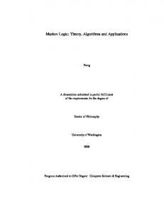
(a) (b) Figure 3: Performance of (a) Prefetch-efficient and (b) Random Matrix Transpose with increasing M/B (Note that scales are different) We performed three sets of experiments with the optimal I-O model matrix transpose. In the first set, prefetching was disabled and the algorithm picked the B × B sub-matrices in a random order. For the second set, the same algorithm was run with prefetching enabled. In the third set, the algorithm had a prefetch-efficient order (i.e. it was aware of the prefetching order and read the sub-matrices to match this order). We found that the first two sets showed no statistical difference with the second set performing marginally better in a few cases. Hence, we report only the second and third set of experiments. One may note that the random ordering of sub-matrices (Set 2), even though optimal in traditional I-O models ([?]), is not implemented in practice. We use such an 13
210000
4e+07
2-way Rebalanced Sort 2-way Sort
200000
M/B-way Sort 2-way Sort (No Prefetching)
3.5e+07
190000 3e+07
I-O Time(ms)
I-O Time(ms)
180000 170000 160000 150000
2.5e+07
2e+07
1.5e+07
140000 1e+07 130000 5e+06
120000 110000
0 500
1000
1500
2000
2500
3000
3500
500
M/B
1000
1500
2000
2500
3000
3500
M/B
(a) (b) Figure 4: Performance of (a) 2-way and (b) M/B-way Mergesort with increasing M/B ordering to demonstrate the inability of I-O models to differentiate between algorithms that have very different I-O times on real systems. Note that the I-O model predicts the running time of all the 3 sets as the running time of second set but it is clear (Fig. 3) that prefetch-efficiency makes a huge difference in performance. In fact, the performance improvement (ratio of Prefetch-Unaware disk I-O time to prefetch-efficient disk I-O time) is fairly close to the maximum achievable theoretically for this disk. The disk can prefetch up to 282 blocks ahead and hence the performance improvement due to prefetching alone is bounded by 282. However, random block accesses not only leads to more disk accesses but the cost of each disk access is also higher. We looked at the logs generated by DISKSIM and noticed that average positioning time for random block accesses is higher than that for prefetched access. Hence, we notice that the performance improvement even exceeds the bound of 282 for large m. One may also note that prefetch-unaware algorithms (Fig. 3 (b)) fails to improve the performance with additional memory since they do not use it for prefetching, whereas we use it to hide the latency of more blocks. To evaluate the impact of prefetching on sorting, we studied the M/B-way mergesort that is optimal in the number of I-Os ([?]) but oblivious to prefetching. We compared it with the performance of our proposed 2-way mergesort that dynamically rebalances data and the standard 2-way mergesort. Prefetching was enabled for all the three algorithms. As a control experiment, we ran a prefetch-disabled 2-way mergesort (2-way sort with prefetching disabled). We observed that both the prefetch-enabled 2-way mergesorts comprehensively outperforms the M/Bway mergesort (Fig. 4). Note that the performance improvement for sorting does not approach the bound of 282. This is because 2-way mergesort performs more I-Os than the M/B-way mergesort. For the chosen value of parameters, a 2-way mergesort performs about 10 times more I-Os than M/B-way mergesort (evident from I-O time of Prefetch-disabled 2-way mergesort (Fig. 4(b)) as well). Hence, even though a 2-way mergesort has to perform a much larger number of I-Os, prefetching is not only able to compensate for it but allows it to outperform the prefetch-unaware algorithm by a significant margin. We also noticed that the average positioning time for disk access for the algorithms are almost same. Hence, prefetching alone attributes for the performance improvement of the 2 − way sorting algorithm. We note that even the standard 2-way mergesort approaches the behavior of the rebalanced sort we propose and comprehensively outperforms the M/B-way mergesort. This is attributed to the fact that the simple 2-way mergesort naturally uses the sequential prefetching present in disks due to readahead caches. This may be an explanation as to why the naturally prefetch-efficient standard 2-way mergesort performs better than the more sophisticated prefetch-unaware M/B-way mergesort on many real systems.
6
Limited Prefetching
In the earlier sections we had assumed that there are no limitations on prefetching. The assumption keeps the model simple but is not consistent with existing architectures. To account for the fact that there are a limited number of prefetch buffers available, we enhance the prefetch model as follows to get a limited prefetch model. We denote by PB the number of blocks that can be prefetched, where PB ≤ M/B. A block si is kept in the prefetch buffer until there is a read request for si , at which time the buffer is released and the block is available in fast memory.
14
6.1
Lower Bounds in the Limited Prefetch Model
We consider the following two cases: (i) L < PB BM and (ii) L > PB BM . Let us assume that A is an optimal algorithm (exact optimal) that performs k I-O in some sequence S. We divide the sequence into (k/PB ) PB − blocks. It is easy to see that the following Lemma holds. Lemma 6. If a block si , s.t. si is the first block of the j th PB − block, is read at time T , then the first block sm of the (j + 1)th PB − block would be available at time no earlier than T + L. Proof: The proof is immediate from the fact that there are only PB prefetch buffers available and the prefetch of sm can be started only after the prefetch buffer used by si is freed. Since that time is T , sm will be available only at time T + L or later. Hence, the time to read any PB − block, other than the first PB − block, is given by max{L, PB BM }. The lemma yields the following general theorem for I-O time. Theorem 11. For any algorithm A that needs k I-Os, kBM > L, the total I-O time needed is Ω(max{ PBLBM , 1}kBM ). The bounds for the specific problems under consideration can be obtained by attaching a multiplicative factor of max{ PBLBM , 1} to the bounds of Theorems (1, 2, 3).
6.2 6.2.1
Running Time in the Limited Prefetch Model Straight Line Algorithms
Case (i):L < PB BM Consider the proof for Theorem 6 and assume that M = PB BM . The implicit assumption in the proof is M = PB BM and we also need the fact that M > L. Since PB BM > L, the assumption still holds good and the theorem holds. Similarly, the corollaries of the theorem hold as well. As a result, all the algorithms that are based on Theorem 6 or its corollaries have identical bounds as shown with unlimited prefetching. Case (ii): L > PB BM This is the more interesting case. We restate Lemma 2 and note that the same proof holds in this setting as well. Lemma 7. For any I-O optimal sequence-preserving straight-line algorithm A, there exists a sequence-preserving algorithm A′ such that if a write of block si of slow memory is made at time t, the read to block si of slow memory is made after at least M/B block I-Os. Also, A′ performs no more I-Os than A and hence is also I-O optimal. For simplicity we assume that PB divides M/B. The time to read a M/B − block other than the first is given MB L by max{L M/B PB , PB PB BM }. Hence, the total time to read k blocks, kBM > L, is given by kBM max{ PB BM , 1}, which matches the lower bound given by Theorem 11, i.e., Theorem 12. A sequence preserving straight line algorithm that uses k I-Os takes total I-O time Θ(kBM max{
L , 1}) PB BM
(16)
Along the lines of Theorem 6, Theorem 12 has the following corollaries. Corollary 4. A sequence of k pre-determined reads, k ≥ M/B, takes time O(kBM max{ PBLBM , 1}). Corollary 5. A sequence of k pre-determined reads and writes, k ≥ M/B, such that no writes follow reads, i.e., there does not exist a pair I1 , I2 ∈ {I w,i , I r,i }s.t.I1 < I2 for some i, takes time O(kBM max{ PBLBM , 1}). Applying Theorem 12 and its corollaries for the different problems, we get the following theorem. Theorem 13. The total time needed to permute N records is Θ(max{
N log(1 + N/B) BM L , 1} min{N BM , }) PB BM log(1 + M/B) B
Tight bounds for other straight line algorithms discussed earlier can be obtained similarly. 15
(17)
6.2.2
Merge Sort
For the 2-way merge sort algorithm, we do the following. We assume that M = PB BM . Since the first phase of the merge-sort has straight line I-O and reads every block only once, it is sequence preserving. Hence, the total time for the first phase is L N , 1}) (18) O( BM max{ B PB BM Also PB = M/B, by our assumption. Also, we have the following lemma on exactly the same lines as Lemma 5. Lemma 8. The cumulative latency for any k − block, k ≤ BM A1 and A2 is bounded by max(L − M 2 B , 0).
M 2B ,
that is disjoint from the first M/(2B) − block of
M/B Proof: We only prove the case L > M/B 2 BM and note that if L < 2 BM then it can be shown that the latency is 0 using a reasoning similar to Theorem 6. The exception part of the lemma is to account for the fact that the initial M/(2B) − block of the first A1 and A2 are fetched deterministically and not in the same manner as the remaining blocks. We will analyze the I-O time for those blocks separately. The proof of the lemma is by induction on k. Base Case: k = 1. Let T0 be the time at which the prefetch for the block si is started. The read request for si M would be made no earlier than T0 + MB 2B , as there are M/2 numbers to be read before reading si . Also, note MBM M that si would be available at T0 + L. Hence, the total latency is at most (T0 + L) − (T0 + MB 2B ) = L − 2B . Let us assume now that the hypothesis holds for m blocks 1 ≤ m < M/(2B), i.e., the cumulative latency M Lm ≤ L − MB 2B . We now look at the time Tm+1 at which the prefetch instruction for the (m + 1)th block sm+1 was given. Note that sm+1 would be available at time Tm+1 + L. Also, note that the read to sm+1 would be made at time later th M block than Tm+1 + Lm + MB 2B . Hence, the latency for the (m + 1)
lm+1 i.e., lm+1 i.e., lm+1 + Lm i.e., Lm+1
≤ Tm+1 + L − (Tm+1 + Lm + M ≤ L − Lm − MB 2B MBM ≤ L − 2B M ≤ L − MB 2B
MBM 2B
)
Hence, for the second phase, the following lemma holds. Lemma 9. The cumulative latency of any PB /2 − block is bounded by L − (PB /2)BM . The total time to read (2N/PB ) PB /2 − blocks is then given by 2N/PB (L − (PB /2)BM )
(19)
Straightforward counting along the lines of the proof of Theorem 9 then yields the following theorem. Theorem 14. The total time needed to sort N numbers using 2-way merge sort in a limited associativity model is O(N log N max{1, PBLBM }).
7
Prefetching with limited streams
Throughout this work, we have worked under the assumption that we can start as many streams as we need and the prefetcher would still be able to prefetch accordingly. However, in real systems, the prefetcher can only support a constant number of streams (typically 8 or 16). We now analyze our algorithm in the light of this restriction. We define s as the number of streams that the prefetcher can support. We first have the following results on the lines of Theorem 6. Theorem 15. Any sequence-preserving straight-line algorithm that accesses s or less streams and uses k I-Os has an equivalent algorithm that takes I-O time O(L + kBM ). 16
Recapitulate that the matrix transpose algorithm uses B streams. Hence, if B ≤ s, the result for matrix transpose holds directly. If B > s, then the same algorithm would run in O(N/B)BM ⌈B/s⌉). This simplifies to O(N/s)BM if B = xs for some x ∈ N. Consider a slight modification of the matrix transpose algorithm where we read M/B records of a row at a time. We then read M/B records of the next row until the memory is full. Note that this would take time O(B(L + M/B 2 BM )) to read M/B blocks. It yields the same N BM /B bound if c(M/B)BM > LB, for some constant c, which is typically the case in many architectures. In the case of sorting, if s ≥ 2 (which is typically the case), the results hold without any modification to our algorithm. We now consider the more difficult cases where we access more than a constant number of sequences. We discuss the case of permutation in a way such that all the other algorithms accessing M/B sequences are also covered. As seen in our experiments, algorithms that are prefetch efficient typically outperform other algorithms that may require fewer I-Os. A case in point are the 2-way merge sort and the M/B-way merge sort where the 2 − way merge sort prefetched O(log M/B) more I-Os. Using this insight we modify all our algorithms that access M/B sequences to read s sequences at any given time. This ensures that Theorem 15 holds and we can prove the following result along the lines of Theorem 7. Theorem 16. The total time required to permute N records is Θ(min{N BM ,
8
N log(1 + N/B) BM }) log(1 + s) B
(20)
Associativity in the Prefetch Model
Throughout the earlier sections, we have assumed that we have full control over the fast memory. This is true when the fast memory consists of registers. Also, if the fast memory is a cache with high degree of associativity, the algorithms can be directly used. We now show that even with small associativity a, the performance of our algorithms do not suffer. Definition 6. We define an algorithm A to be accessing k sequences if A loads data from a set Il of k different non-contiguous locations called index locations. Also, all other accesses by A are part of a sequential access from some index location in Il . To recapitulate, the data access pattern of all our algorithms can be divided into the following two categories. • Accessing 2 sequences: The 2-way merge sort algorithm falls in this category • Accessing M/B sequences: The remaining algorithms discussed fall in this category. We will now show that limited associativity does not increase the running time for the first case. For our algorithms that fall in the second category, we use the technique of [?] to modify them and show that the expected running time does not increase by more than a constant factor. Lemma 10. If a ≥ 2, there are no conflict misses in reading 2 sequences, where each sequence is stored contiguously in slow memory. Note that we have not considered the conflict misses incurred because of the cache used in writing out the merged sequence. This is because current architectures support instructions that allow an algorithm to write to a memory location without getting the data into cache [?]. In such a scenario, writing back is independent of cache. However, if that architectural feature is absent, then the Lemma holds for a ≥ 3. The above lemma directly leads us to the following theorem. Theorem 17. In a cache-memory model that supports prefetching, if a ≥ 2 then 2-way merge sort takes time O( BBM N log N ). For the M/B case, we first state the technique and results of Mehlhorn and Sanders [?] that can be applied to this case. Mehlhorn and Sanders [?] consider the problem of scanning multiple sequences, where a pointer into each sequence is maintained. An adversary specifies which pointer is to be advanced. They show that by randomizing the starting addresses of the sequences, the number of conflict misses can be kept to O(N/B), provided the number of sequences, k = O(M/B (1+1/a) ). The exact constant depends on the degree of associativity. With minor modifications, we obtain the following result. 17
1/a
Theorem 18. If (M/B)BM ≥ LBc1 total time to permute N records is
for some constant c1 and M ≥ B
Θ(min{N BM ,
a+c2 a
for some constant c2 > 1, then the
BM N log(1 + N/B) }) B log(1 + M/B)
(21)
Proof: We argue that the technique of Mehlhorn and Sanders can be applied to our problems by increasing the amount of slow memory and the running time. The only cause for concern is that k is smaller than M/B by a factor of B 1/a . We will argue later that this does not increase the running time in most practical scenarios. For now, we look at the modified algorithm that reads at most M/B (1+1/a) sequences at any time. Note that our algorithms would then use only M/B 1/a amount of memory instead of M . As a consequence, the I-O time per unit of data is given by LB 1/a B BM } (22) max{1, B M BM The above is obtained by arguing that for pre-determined reads, the maximum of L and (M/B (1+1/a) )BM time is needed for reading M/B 1/a units of data. Hence, the effective time to transfer one unit of data is 1/a
L max{ BBM M/B , } instead of BM /B, as achieved from Theorem 6 by using the fact that k ≥ M . However, M/B 1/a M/B 1/a this change in the algorithm ensures that the merge degree (k) is sufficiently small for Sanders’ result [?] to be applied. Moreover, the following properties hold for the algorithm.
• Only one block per sequence is in fast memory at any time. • The location of each block in fast memory is known a priori. • The conflict misses can be worked out a priori for straight-line algorithms. The first condition implies that we can apply Sanders’ result directly. The second and third conditions imply that the sequence of I-Os required (including even those needed because of the conflict misses) are known a priori. Hence, the total I-O time can be computed by computing the number of I-Os required, computing the IO time in the prefetch model from it and then multiplying by the factor given in Eqn. 22. The total running time for permuting using the M/B-way merge sort is then given by BM log N/B − 1/a log B LB 1/a B }O(N max{1, ) B M BM log M/B − 1/a log B
(23)
In any practical system, B is usually a small constant and it can be safely assumed that M ≥ LB 1/a and a+c M ≥ B a for some constant c > 1. Putting these two conditions into Eqn. 23 would give the same bound for permuting as obtained without considering associativity in Eqn. 5. Note that the naive algorithm for permuting reads only one element of a block. Hence, it never incurs any conflict misses and therefore the bound for the naive algorithm does not change at all. We have only provided the results for permuting with limited associativity and note that algorithms for the other problems that access M/B sequences can be similarly modified and the corresponding bounds obtained.
9
Discussion
We have presented an I-O model that incorporates prefetching and presented simple algorithms for many common problems that are optimal in this model. We provide insights that relate the prefetch model with the familar PDM model and use them to design an emulation technique to develop algorithms optimal in prefetch model from optimal PDM algorithms. For specific problems, the algorithms presented have similarities with optimal algorithms in the cache-oblivious model as well. A familiar case is Matrix Transposition, where the optimal cacheoblivious algorithm [?] can be made to work in the prefetch model by introducing a base case in the recursion that prefetches all data if the size of the matrix is less than or equal to M . Note that this makes the algorithm cache-aware but it allows us to prefetch O(M ) data at the same time and hide the latency for M/B blocks, thus making it prefetch-efficient. Similarly, the cache-oblivious funnelsort algorithm [?] can be made to work optimally in prefetch-model by adding a base case in the recursive merger to use the dynamic rebalancing of data proposed for constant way merging, if the number of runs being merged is a constant. However, usage of the dynamic 18
rebalancing technique makes the algorithm cache-aware. Whether the two models have any essential similarity or not that can lead to a general emulation technique is still an open problem. Another important direction of future research is identifying the number of streams s (Sec. 7) supported by the underlying hardware. In a cache-RAM model, an explicit parameter specifies s. In a modern disk, s is lower bounded by the number of readahead cache segments (which is small). However, usage of schedulers like SCAN potentially increases the number of streams since careful use of prefetch instructions by the algorithm may allow SCAN to support multiple prefetch streams in the same cache segment. We believe the number of supported streams s is most important parameter in the extended prefetch model and hence, characterizing s for a modern disk is an interesting direction for future research.
10
Acknowledgement
The authors would like to thank Dr. Rahul Garg for valuable discussions on formulation of prefetch model.
19
A A.1
Appendix I-O Model results
Lemma 11. The worst-case number of I-Os required for sorting N records and for computing the N -input FFT digraph or an N -input permutation network is Θ(
N log(1 + N/B) ) B log(1 + M/B)
(24)
Also, there are permutation networks such that the number of I-Os needed to compute them is O(
N log(1 + N/B) ) B log(1 + M/B)
(25)
Lemma 12. The worst-case number of I-Os required to permute N records is Θ(min{N,
N log(1 + N/B) }) B log(1 + M/B)
(26)
Lemma 13. The number of I-Os required to transpose a matrix with p row and q columns stored in row-major order, is N log min{M, 1 + min{p, q}, 1 + N/B} ) (27) Θ( B log(1 + M/B) Further, if M > B 2 then the total number of I-Os required are Θ(N/B).
20