nodes maintain a list of kNN which indicate the outgoing edges of the graph; ... The kNN-Graph for a set of objects is a directed graph with vertex set R ⪠S and.
Boundary Points Detection Using Adjacent Grid Block Selection (AGBS) kNN-Join Method Shivendra Tiwari, Saroj Kaushik Department of Computer Science and Engineering IIT Delhi, Hauz Khas, New Delhi, India 110016 {shivendra , saroj}@cse.iitd.ac.in
Abstract. Interpretability, usability, and boundary points detection of the clustering results are of fundamental importance. The cluster boundary detection is important for many real world applications, such as geo-spatial data analysis and point-based computer graphics. In this paper, we have proposed an efficient solution for finding boundary points in multi-dimensional datasets that uses the BORDER [1] method as a foundation which is based on Gorder knearest neighbors (kNN) join [10]. We have proposed an Adjacent Grid Block Selection (AGBS) method to compute the kNN-join of two datasets. Further, the AGBS method has been used for the boundary points detection method named as AGBS-BORDER. It executes AGBS join for each element in the dataset to get the paired (qi, pi) kNN values. The kNN-graphs are generated at the same time while computing the kNN-join of the underlying datasets. The nodes maintain a list of kNN which indicate the outgoing edges of the graph; however the incoming edges denote the Reverse kNN (RkNN) for the corresponding nodes. Finally, threshold filter is applied - the node whose number of RkNN is less than the threshold values are marked as the border nodes. We have implemented both the BORDER [1] and AGBS-BORDER methods and tested the same using randomly generated geographical points. The AGBS based boundary computation over performs the existing BORDER method. Keywords: k-Nearest Neighbor (kNN), Reverse kNN (RkNN), kNN-Join,, Cluster Boundaries, Principal Component Analysis (PCA), Adjacent Grid Block Selection (AGBS).
1 Introduction The size of spatial database increases dramatically and the structure of data becomes more and more complicated. To discover valuable information in those databases, spatial data mining techniques have been paid significant attention during recent years. Knowledge discovery in databases is a non-trivial process of identifying valid, interesting and potentially valuable patterns in data. Due to the need for efficient and effective analysis tools to discover information from these data, many techniques have been developed for knowledge discovery in databases. Such techniques include data classification, mining association rule, clustering, outlier analysis, data cleaning and data preparation. In general, clustering is a method to separate data into groups
without prior labeling so that the elements inside the same group are most similar [1]. The cluster boundary detection is becoming more and more valuable for many real world applications, hence it is important to optimize the boundary detection algorithm as much as possible. Mostly, the boundary point detection algorithms scan the complete data space iteratively and therefore computation cost happens to be high. Even the small improvement in the memory and computation results a significant impact on the overall systems [5]. The kNN algorithm is a method for classifying objects based on closest training examples in the feature space. A kNN of a data point rR is a set of k points sS which are closest among the rest of the points s’S. The kNN join between two datasets R and S, returns the kNN points ps S for each point pr R. The kNN-Join is important as the one-time computation of the neighbors for all data points can dramatically accelerate the operations of the traditional one-point-based similarity search. For example, data mining algorithms can be implemented on the top of one join operation, instead of many similarity queries. However computing the kNN Join iteratively for the dynamic and changing data is expensive. Essentially, the kNN-join combines each point of the outer dataset R with its kNN from the inner dataset S. The applications of the kNN-joins include kNN classification, k-means clustering, sample assessment and sample post-processing, k-distance diagrams, etc [3]. We assume a metric space and the objects are represented by a multidimensional point in the space. Therefore, we also refer to an object as a point occasionally. A data point in our context is a multidimensional feature vector corresponding to a complex object such as an image. In the rest of the paper, we use R to symbolize the outer dataset and S the inner dataset.
Fig.1. kNN Graph for k=3. The outgoing edges show the kNN relationships; however the incoming edges denote the RkNN relationships among the data points.
The kNN-Graph for a set of objects is a directed graph with vertex set R S and an edge from each r R to its k most similar objects in S under a given similarity measure as shown in Fig.1. The nodes in the graph represent the data points labeled as Pi. Each node keeps record of their incoming and outgoing edges. The kNN-graphs are useful on the various cluster analysis processes.
The kNN cluster can be divided into three parts i.e. Core, Ourlier, and Boundary points. A Core Point is defined as a point that has at least k RkNN points: i.e. |RkNNs| ≥ k. An Outlier Point is a point that has less than k number of RkNNs i.e. |RkNNs| < k. Lesser the number of RkNNs, the more distant it is from its neighbors. A Boundary Point is an outlier, classified to be boundary point, if majority of its RkNNs belong to one cluster. Boundary points are data points that are located at the margin of densely distributed cluster. The difference between Boundary Point and Outlier Point is that a boundary point is one that is usually near the boundaries of a cluster or amidst more than one cluster; however an outlier point has |RkNNs| < k and most of its RkNNs are outliers. But for a boundary point, its |RkNNs| < k and most of its RkNNs are core-points [1]. In order to filter unnecessary distance computation in the kNN-join processing, popular algorithms based on an index such as the R-tree compute the MinDist (i.e. minimum distance between the query point and a node of the R-tree) and choose to traverse the node with the minimum MinDist first. The MinDist is also compared with the pruning distance (the distance between the query point and its kth nearest neighbor candidate). Our work-in-progress AGBS’s efficient grid creation, grid block searches, nested block join scheduling have been used for the boundary points detection in this paper. This paper is divided into six sections. Section 2 and 3 contain the related work and AGBS based kNN-join computation method separately. Section 4 explains the efficient AGBS-BORDER algorithm for the boundary points detection. The sections 5 and 6 talk about the cost analysis, limitations & future work respectively. Finally the paper has been concluded in the section 7.
2 Related Work There has been a considerable amount of work on efficient nearest neighbor finding methods [10, 12, 14, and 15]. The reverse k-nearest neighbor (RkNN) problem has been first proposed in 2000 [4] and has been paid increasing attention to in the recent years. Existing studies all focus on the single RkNN query. Various methods have been proposed for its efficient processing and can be divided into two categories: precomputation methods and space pruning methods. The shortcoming of precomputation methods is that they cannot answer an RkNN query unless the corresponding k-nearest neighbor information is available. The preprocessing of knearest neighbor information is actually a kNN join. Space pruning methods utilize the geometry properties of RkNN to find a small number of data points as candidates and then verify them with nearest neighbor queries or range queries. Space pruning methods are flexible because they do not need to pre-compute the nearest neighbor’s information. However, they are very expensive when data dimensionality is high or the value k is big. In 2008, Dongquan Liu et al proposed a boundary detection algorithm known as TRICLUST based on the Dalaunay Triangulation [5]. TRICLUST algorithm treats clustering task by analyzing statistical features of data. For each data point, its values of statistical features are extracted from its neighborhood which effectively models
the data proximity. By applying specifically built criteria function, TRICLUST is able to effectively handle data set with clusters of complex shapes and non-uniform densities, and with large amount of noises. One additional advantage of TRICLUST is the boundary detection function which is valuable for many real world applications such as geo-spatial data processing, point-based computer graphics, etc. Since we are mainly interested in spatial data which is usually low dimensional, the analysis here is for two dimensional cases. The time complexity of constructing Delaunay triangulation graph is O(N.logN), where N is the number of data points. Olga Sourina et al proposed a clustering and boundary detection method for the time dependent data in 2007. The method is based on geometric modeling and visualization. Datasets and boundaries of clusters are visualized as 3D points and surfaces of reconstructed solids changing over time. This method applies the concepts of geometric solid modeling and uses density as clustering criteria that comes from traditional density-based clustering techniques. Visual clustering allows the user to analyze results of clustering the data changing over time and to interactively choose appropriate parameters [11]. The set oriented kNN-join can accelerate the computation dramatically. The MuX kNN-join [12] and the Gorder kNN-join [10] are two up-to-date methods specifically designed for kNN-join of high-dimensional data. MuX is essentially an R-tree based method designed to satisfy the conflicting optimization requirements of CPU and I/O cost. It employs large-sized pages (the hosting page) to optimize I/O time and uses the secondary structure, the buckets which are MBRs (Minimum Bounding Rectangles) of much smaller size, to partition the data with finer granularity so that CPU cost can be reduced. MuX iterates over the R pages, and for R page in the memory, potential kNN-joinable pages in S are retrieved through MuX index on S and searched for knearest neighbors. Since MuX makes use of an index to reduce the number of data pages retrieved, it suffers as an R-tree based algorithm and its performance degrades rapidly when the data dimensionality increases. Gorder kNN-join [10] is a non-index approach. It optimizes the block nested loop join with efficient data scheduling and distance computation filtering by sorting data into the G-order. The dataset is then partitioned into blocks that are amenable for efficient scheduling for join processing and the scheduled block nested loop join is applied to find the k-nearest neighbors for each block of R data points [1]. The block selection in Gorder [10] is a brute force search and also the size of the blocks does not consider the value of k. Chenyi Xia et al further used Gorder for boundary point’s detection in 2006 known as BORDER [1]. It processes a dataset in three steps. First, it executes Gorder kNN join to find the k-nearest neighbors for each point in the dataset. Second, it counts the number of reverse k-nearest neighbors (RkNN number) for each point according to the kNN-file produced in the first step. Third, it sorts the data points according to their RkNN number and finally, the boundary points whose RkNN number is smaller than a user predefined threshold can be incrementally output [1]. However it still goes through the multiple steps that need additional memory and computation cost. We have studied latest kNN-Join algorithms and are proposing a better algorithm based on the adjacent block selection and nested block scheduling methods in the following section.
3 Computing kNN-Join with Adjacent Grid Based Selection The adjacent grid block selection based kNN join method is based on the fact that the grid cells are surrounded by the adjacent neighboring cells which are the priority candidates of the kNNs for the query points in a block. There are two steps of the algorithm i.e. preprocessing of the datasets and the kNN-join operation. The preprocessing of the data includes two major operations – the principal component analysis (PCA) [10, 20] as shown in Fig. 2 and the grid block generation. In the kNNjoin phase, we use the physical adjacency of the grids to select the block for the computation.
Fig.2. Illustration of the Principal Component Analysis
3.1 Preprocessing of Datasets Before the kNN-join operation takes place, the dataset is prepared in such a way that the I/O and CPU costs are minimized. The PCA (principal component analysis) transformation and the Grid Block Generation are the two major preprocessing steps in the AGBS method. In Algorithm 1, the grid blocks are generated for both of the datasets if the operation is not self-join i.e. both the datasets are not the same. Algorithm 1 Preprocessing (R, S) Input: R and S are two data sets. Description: Principal-Component-Analysis (R, S); Grid-Block-Gen(R); If R!=S then
Grid-Block-Gen(S);
3.1.1 Principal-Component-Analysis Principal component analysis (PCA) is a standard tool in modern data analysis and data mining. It is a simple and non-parametric method for extracting relevant information from confusing data sets. With minimal effort PCA provides a roadmap for how to reduce a complex data set to a lower dimension to reveal the sometimes hidden, simplified structures that often underlie it [20]. After applying PCA processing, most of the information in the original space is condenses into the first few dimensions along which the variances in the data distribution are the largest. The first principal component (or dimension) accounts for as much of the variability in the data as possible, and each succeeding component accounts for as much of the remaining variability as possible as shown in Fig 2 [10]. 3.1.2 Grid Block Generation The grid block generation for given dataset is based on the two major considerations i.e. the bigger block should be used for the I/O and the smaller blocks should be used for distance computation. Since the most of the computation cost arise in the distance computation at the data level, the data blocks should be of optimal size on the runtime memory. If we assume each block as a kNN cluster, it will need at least k data points into it to satisfy all the points. It needs to compute the distance between at least k points in order to find the kNN of a single point. Hence the complexity of the kNN join can not be less than the O(nk). We propose to ensure the average number of points in a single lowest level block to be O(k). Since the distance computation has been minimized at the data point’s level, the computation cost is expected to increase at the grid block selection. The optimization in the block selection technique will improve the overall performance of the system. The idea is to create multilevel grid block hierarchy of the input datasets. First, divide the data into the bigger blocks in the secondary storage. The blocks have specific identity that can be used for the search at the time of join operation. A multilevel index file can be created separately to store the block id and their offset in the file mappings. The secondary storage blocks are read at the time of kNN-join operation selectively. Second, further more levels of grid block hierarchy are created on the memory to reduce the distance computation. The global grid block matrix is loaded on the memory which is lightweight information of the block structure that can be implemented on a multidimensional array. Let’s assume that the Mini and Maxi are the minimum and the maximum values of the ith dimension in the dataset R and the total number of blocks is N. i is the maximum difference of values between any two points of a grid block in the ith dimension. The point values in the nth block of the ith dimension are from (Mini + n * i) to (Min i + (n+1) * i - ). Here, is the threshold value to handle the grid block boundary. Considering the total point count in the dataset R is |R|, then N and i is calculated as below:
| R | N k
(1)
Maxi Mini i N
(2)
Where, k is the value in k-Nearest Neighbor join query. The calculation of the cell id is simply based on the range division of the dataset in question. The blocks are partitioned it into Nd rectangular cells, where N is the number of block per dimension of the grid. Fig. 3 is an illustration of a two-dimensional space partitioned by a 9x9 grid. A vector of block ids for each dimension makes the unique identity of a block or a cell. The block id of the point pr R for the ith dimension can be calculated as below:
p Mini bi i i
(3)
In Algorithm 2, the blocks are generated for the dataset R. All the points in the dataset are iterated, and the grid block identity is calculated. The procedure ComputeBlock-id() in line 2 is used to compute the grid block or the cell id as per the equation (3). There are separate blocks for each dimension in consideration after the PCA processing. Assuming that the block number for the i th block is bi, the cell id is a vector of block numbers i.e. . In line 3, Point-to-Block() procedure is used to divide the data and store the points into the cell at the secondary storage. A multidimensional matrix structure can be used to physically store the points into the grid blocks on the runtime memory. As soon as the runtime memory reaches to the limit the cell data is written into the secondary storage. We propose to create separate files for each data page (I/O optimization block) so that the file seek operations are minimized. Once all the data points are written into the secondary storage blocks, the cells are merged in the sorted order of their block id vector. The search of the appropriate cell is fast being the direct memory access in the matrix. Algorithm 2 Grid-Block-Gen(R) Input: R is a dataset Description: for each point pr R do cell-id = Compute-Block-id (pr); Point-to-Block (pr, cell-id);
3.2 Adjacent Grid Blocks Selection Join In the second phase of this method, the grid blocks of R and S are examined for joining. The two-tier partitioning strategy has been applied to optimize the I/O time
and CPU time separately. The first-tier partitioning is optimized for I/O time. We partition the grid oriented input datasets into blocks consisting of several physical pages. The blocks in dataset R are loaded into memory sequentially and iteratively one block at a time and the S blocks are loaded into memory in the surrounding adjacent sequence based on their similarity to the R data in buffer. The loading of bigger block at a time is efficient in terms of I/O time as it significantly reduces seek overhead. In addition, in order to optimize the kNN processing, it selects the S blocks so that the S blocks that are most likely to yield k-nearest neighbors can be loaded into memory and joined with R data in buffer early. The large block size reduces disk seek time, however, as a side effect; it may introduce additional CPU cost due to redundant pair-wise distance computation of tuples for kNN-join. To overcome such a problem, we use the two-tier partitioning in memory. The two tier hierarchy on memory is of smaller data size called Blocks and Sub-blocks.
Fig.3. AGBS Block Traversal in their adjacency neighboring order.
Algorithm 3 Grid-Block-Selection-Join (R, S) Input: R and S are two grid oriented data sets that have been partitioned into blocks. Description: for each block Br R do Read-Block(Br); Find-Closest-Block(S, Br); for each Bs Surrounding-Adj-Block(S, Br) do Read-Block(Bs); Block-Join(Br, Bs); Output-KNN(Br);
Algorithm 3, outlines the join algorithm of AGBS method. It loads secondary storage data blocks of R into memory sequentially. For the R block in memory B r, S blocks are selected in the increasing order of their adjacency to Br. With each pair of R and S block, we join them in memory by calling function Block-Join(). After all unpruned S blocks are processed with Br, the kNN points are written into the output files. Algorithm 4 Block-Join (Br, Bs) Input: Br and Bs are the grid blocks that have been partitioned into more sub-blocks further on memory. Description: for each sub-block SBr Br do Find-Closest-Block(Bs, SBr); for each SBs Surrounding-Adj-Block(Bs, SBr) and SBs NotPruned(Bs, SBr)do Sub-Block-Join(SBr, SBs); In Algorithm 4, the data is available on memory to be processed. SBr Br is the sub-blocks divided based on the data density and the k value in the query. For each sub-blocks SBr, the Find-Closest-Block() method finds the closes sub-block SBs Bs. Then the surrounding sub-blocks in Bs are selected in the increasing order of their adjacency to SBr. With each pair of SBr and SBs block, the join operation takes place in runtime memory by calling function Sub-Block-Join(). Algorithm 5 Sub-Block-Join(SBr, SBs) Input: SBr and SBs are two sub-blocks from R and S respectively. Description: for each point pr SBr do if(MinDist(pr,SBr)