QUT Digital Repository: http://eprints.qut.edu.au/
Agha Zadeh, Ramin and Ghosh, Arindam and Ledwich, Gerard (2010) Combination of Kalman filter and least error square techniques in power system. IEEE Transactions on Power Delivery, 25(4). pp. 1-13.
© Copyright 2010 IEEE
Review Copy: IEEE Transactions on Power System.
1
Combination of Kalman Filter and Least Error Square Techniques in Power System Ramin Agha Zadeh, Student Member, IEEE, Arindam Ghosh, Fellow, IEEE, Gerard Ledwich, Senior Member, IEEE Abstract—An algorithm based on the concept of combining Kalman filter and Least Error Square (LES) techniques is proposed in this paper. The algorithm is intended to estimate signal attributes like amplitude, frequency and phase angle in the online mode. This technique can be used in protection relays, digital AVRs, DGs, DSTATCOMs, FACTS and other power electronics applications. The Kalman filter is modified to operate on a fictitious input signal and provides precise estimation results insensitive to noise and other disturbances. At the same time, the LES system has been arranged to operate in critical transient cases to compensate the delay and inaccuracy identified because of the response of the standard Kalman filter. Practical considerations such as the effect of noise, higher order harmonics, and computational issues of the algorithm are considered and tested in the paper. Several computer simulations and a laboratory test are presented to highlight the usefulness of the proposed method. Simulation results show that the proposed technique can simultaneously estimate the signal attributes, even if it is highly distorted due to the presence of non-linear loads and noise. Index Terms—Frequency estimation, amplitude estimation, phase angle estimation, Kalman filtering, Least error square, harmonics, noise, nonlinear loads
C
I. INTRODUCTION
ONTROL and protection of power system is critically dependant on real time estimates of signal attributes. The faster and more precise are the estimates, the more reliable are the applied control and protection schemes. Harmonic and noise contamination have become a major concern for power system since they affect the accuracy of the estimates and the speed of estimation. In addition, the integration of power electronic devices to utility grids necessitates the presence of such a reliable estimator that not only provides service to linear loads but also compensates/caters for nonlinear loads. Various techniques have been introduced in the literature to measure the signal attributes. Discrete Fourier transform (DFT) and its modifications [1,2,3], Kalman filtering [4,5,6], phase locked loop (PLL) [7], least square (LS) [8,9], Newton type algorithms [10], and adaptive notch filters [11] are among the existing techniques. Most of these techniques do not provide comprehensive estimation results including all attributes of signal (frequency, amplitude, and phase angle) for both funManuscript submission date: July 20, 2009. R. Agha Zadeh, A. Ghosh, and G. Ledwich, are with the School of Engineering Systems, Queensland University of Technology, Qld 4001, Australia (e-mail addresses:
[email protected];
[email protected];
[email protected];
[email protected] ).
damental and harmonic components. References [5,12-15] review these techniques and outline the strengths and drawbacks of each of them. Noise and the distortion of signal are issues that these techniques have considered. Although, they have suggested some solutions for taking care of these issues, still the results can be improved especially by using new algorithms implemented in state-of-the-art microprocessors. A literature review shows that PLL based techniques have been proved to have desirable performance in tracking the attributes of the fundamental component [12,16-19]. Reference [15] analyzes the performance of the PLL and highlights the tracking errors derived due to distortion such as phase unbalancing, harmonics, and offset. References [12,16,17] have mitigated the effects of harmonics and noise pollution using enhanced methods of the PLL approach. However, these techniques focus on the attributes of the fundamental component rather than on harmonic components. Techniques such as Prony's method [20,21], ESPRIT [22], Root-MUSIC [23], and frequency-domain interpolation method [24] provide good results for the signals with wide spectrums especially when the inter-harmonics are involved. Theses techniques provide significant estimation results although at the expense of large computation loads and considerable delays. Kalman-filter based techniques, extended or enhanced with frequency estimation algorithms, can provide comprehensive results comprising of the attributes of fundamental and harmonic components as well as dc-offsets [14]. Nonetheless, in order for the Kalman filter to maintain the variance of the estimation error as low as possible, the specific statistical settings about disturbances and noise must be chosen close enough to realty. Lowering the level of disturbance and noise leads to less deviation between these settings and the real values. Therefore, this paper proposes a method that the input signal is refined before being fed to the Kalman filter. Another drawback of Kalman filtering is its weak response to large changes in the signal parameters. To rectify this, a technique is proposed to detect these critical changes and then apply a different estimation technique, so-called enhanced LES. However, the LES method is used only in the critical transients. In fact, Kalman filtering is the main estimator in the steady state and non-critical transients as it requires less computational effort and can give better or even optimal results provided the statistical settings are proper or exact. The other contribution of the paper is to propose a method to provide the Kalman filter with relatively accurate estimates of system frequency.
Review Copy: IEEE Transactions on Power System.
2
This paper is organized as follows. In Section II, the proposed algorithm is derived. The analysis of the proposed technique calls for some crucial parameters and relevant computation effort. The consequences of these issues and recommended solutions are explained in Section III. The performance of the proposed method is evaluated in Sections IV and V. Section VI summarizes the main conclusions of the paper. II. DEVELOPMENT OF THE ALGORITHM A typical power system or power electronic signal can be expressed as follows. v (t ) a1 sin 2 ft 1 h t n t v d
(1)
where symbols h(t), n(t) and vd represent the harmonic, noise and offset parts of the signal, respectively. The signal offset is often produced in the measurement and data conversion process using A/D devices. The signal is theoretically modeled in this paper as the combination of the fundamental component, odd harmonics up to the 9th order and the offset component. It is assumed that necessary low-pass filters exist in the power system that harmonics higher than the ninth order are unaccounted for in the signal model. Also, inter-harmonics with non-integer orders are not in the scope of this paper. The modeled signal can then be summarized as y (t )
5
a k 1
2 k 1
sin 2 k 1 t 2 k 1 v d
(2)
The sampling rate chosen here is 80 kHz. Thus, the sampling interval, denoted by ∆T in this paper, is 12.5μs. A. Frequency Estimation Algorithm The basic sub-algorithm in [14,25] called “sample counting and interpolation technique” is enhanced here to be used for the purpose of frequency estimation. If a zero crossing takes place between the two consecutive samples of a signal such as Si-1 and Si or at the leading sample, Si, the frequency can be calculated in the following manner. 0 .5 (3) fj p 1 T j j where p denotes the number of samples located between two consecutive zero crossings. It should be noted that values of p less than 0.9pu or more than 1.1pu will be rejected to avoid inaccurate frequency estimation due to multiple zero crossing or large phase angle steps. Also, the correction factors αj and βj are calculated in [14] as functions of Si-1 and Si. In this paper Si-1 and Si are defined in the following manner. Si
2w
y k 0
(4)
ik
Let us define the following relations. i i ti , xi i T Ak a k sin k i k , B k a k cos k i k i
k 1 2 cos krx r 1
4
S i 1 A1i w 2 k 1 A 2 k 1 i w 2 w 1v d
(7)
k 1
It can be shown that the signal S(t) whose digital samples are expressed as Si, is periodical with the same period as y(t). Finally, the correction factors can be calculated using following condition: If Si×Si-1 ≤ 0 and Si-1 ≠ 0, then j 1 S i T /( S i S i 1 ) j 1 j 1
(8)
B. Amplitude and Phase Angle Estimation by Kalman filter In this section, a modification to the conventional Kalman filter is proposed to estimate the amplitude and phase angle of the preprocessed signal. The reason to preprocess the input signal is shown in the Appendix. It can be shown that preprocessing leads to a considerable decrease in the settings for the level of noise. According to (7), the relevant state vector components are similar to the conventional ones but they all are weighted by λk coefficients defined in (6). Therefore, the 11×1 state vector must be defined as m 1, 3, 5, 7 , 9 m Bmi 2 w 1 w (9) X i ( m ,1) m 1 Am 1 i 2 w 1 w m 2, 4, 6 , 8, 10 m 11 2 w 1 v d It can be shown that the following relation is valid for the state vector. X i 1 F x X i (10) diag .[ f x , f 3 x , f 5 x , f 7 x , f 9 x ,1] X i where diag. denotes the diagonal element of F based on the following square matrix. It should be noted that x'=(2w+1)ω∆T. Thus, the computation cycle time given to the modified Kalman filter is (2w+1) times larger than the sampling interval. This can also help to maintain the white sequence of noise in the samples of Si fed to the modified Kalman filter. cos[( 2 k 1) x ] sin[( 2 k 1) x ] (11) f [( 2 k 1) x ] sin[( 2 k 1) x ] cos[( 2 k 1) x ] The Appendix describes briefly the details of the Kalman filter and more importantly explains how the statistical information of the disturbances must be prepared for the Kalman filtering. However, matrix H and vector Z are arranged as follow. Z i HX i [0,1, 0,1, 0,1, 0,1, 0,1, 1] X i (12) A A A 1
1i 2 w 1 w
3
3i 2 w 1 w
5
5i 2 w 1 w
7 A7i 2 w 1 w 9 A9i 2 w1 w 2 w 1vd S i 2 w1 (5)
i
w
Therefore, the expansion of (4) according to (2) and the relations defined in (5) and (6) can give the following equation.
(6)
Let us define the following relation. (13) Y DX where 1 (14) D diag. 11 , 11 , 31 , 31 , 51 , 51 , 71 , 71 , 91 , 91 , 2w 1
Review Copy: IEEE Transactions on Power System. yi yi-1
Sample & Hold
yi
Frequency Estimator
+ yi-2w
Si
3
fi Xi
Kalman Filter
D
Yi
×
Fig. 1. The block diagram of the modified Kalman filter
The amplitude and phase angle of the signal components can be calculated using the components of Y. The proposed estimation process can be summarized in Fig. 1. It is obvious that the proposed modification to Kalman filter is in series with the Kalman filter. Therefore, the stability of the proposed system follows that of the Kalman filter. C. Amplitude and Phase Angle Estimation by LES Let us define the following relations. i i mx t i m T
Aki Ak i m a k sin k i k , B k i B k i m a k cos k i k yi yi m
5
a k 1
2 k 1
yi
5
k 1
k 1
(15)
sin 2 k 1 i mx 2 k 1 v d
5
A k 1
2 k 1 i r
5
a k 1
2 k 1
A k 1
vd
sin 2 k 1 i 2 k 1 rx v d
5
2 k 1 i
(16)
cos rx B 2 k 1 i sin rx v d
Equation (16) can help arrange an LES approach of 2m+1 equations in 11 unknowns. The matrices of the LES system can then be stated in the following manner. (17) Y e Ae X e where the elements of Ae can be obtained in the following manner in accordance with (16). l 11 h , l (18) A h , l e
l 11
1
where: l l 1 h h , l sin l 2 2 1 x 2 2 2 2
(19)
in which: 1
(20)
if l is odd and h is even
1
else
The elements of Xe and Ye at ti are defined respectively as Ahi X ei h ,1 B h 1 i v d
Yei h ,1 y i 1 h
i 1 0 . 5 h m
Ahi m w if h is odd and less than 11 i h ,1 Bh 1i m w elseif h is even and less than 11 (25) elseif h 11 v d Therefore, from (7), (19), (21), and (23) to (25) the elements of U can be derived as follows. l 11 h , l l 1 2 (26) 1 2 U h , l i
5
A2 k 1 i v d A 2 k 1 i m v d
where, 2m+1 is the number of least error square equations while m must be larger than 5 to ensure to have an overdetermined system. From (15), followings can be developed. yir
Anyhow, equation (17) yields unacceptable results because the signal samples constructing the LES input vector are subjected to noise and unaccounted-for harmonic contamination. To tackle this issue, the LES system of (17) can be modified as (23) V U where the elements of modified LES matrices are specified as (24) V i h ,1 S h
if h is odd and less than 11 elseif h is even and less than 11
(21)
elseif h 11
0 .5 h
where 0 . 5 h denotes the integer floor number of 0.5h.
(22)
2 w 1
l 11
It seems that Λ can be solved from (23) and can give precise results due to the noise reduction applied. However, the outcomes are still unacceptable. The reason behind this relates to the method employed by MATLAB for computing sinusoidal functions. Packages such as MATLAB use Taylor series expansion method to calculate the sinusoidal functions. They use a finite number of terms in the series. Thus, unavoidable errors can be produced while dealing with minor magnitudes of sinusoidal functions. Elements of U apart from those in the eleventh column include sinusoidal functions involving tiny arguments. To tackle this problem, let us enlarge the arguments of these sinusoidal functions. Parameter q is used for this purpose and is set to 20. Thereby, the elements of the input vector and transition matrix are modified as follows. (27) V i * h ,1 S i 1 h 0 . 5 h q mq
Ahi mq w if h is odd and less than 11 X h,1 Bh 1i mq w elseif h is even and less than 11 elseif h 11 vd * i
(28)
(29) From (27) to (29) the elements of the transition matrix, B*, can be stated as * h , l l 1 l 11 2 (30) * 1 B h , l 2 V * B* X *
i
2 w 1
l 11
where: l l 1 h * h , l sin l 2 2 1 xq 2 2 2 2
(31)
The elements of X* can yield the amplitude and phase angle components of the signal. However, the consequent estimation delay due to the summation, required as per (27) will be (mq+w)∆T seconds, that has also been considered in (28). D. How to combine the Kalman filter and LES parts
Review Copy: IEEE Transactions on Power System.
4
It can be shown that Kalman filter suffers from a delay about 2.5 cycles in the critical transients where the changes in signal
Fig. 2. Residue ratios [i / r1(i), the black-colored graph, and 'i / r1(i), the graycolored graph]
parameters are relatively large. However, the respective delay of the proposed LES system is less than a half cycle. Therefore, it is necessary to detect these critical transients in the online mode. This can be achieved by monitoring the difference between the real value of the latest signal sample and its predicted value based on the past trend of the signal. The best way is to use the following index for monitoring the condition of signal: (32) u i y i H X i* * * where X i is the predicted estimate of X i , the process-state vector when y(t) is directly fed to the measurement vector of Kalman filter. Therefore, ui represents the difference between the latest sample and its predicted estimate. X i* and X i* can be obtained or updated by the following equations. (33) X i* X i* K i u i * * (34) X i 1 F T X i The index of monitoring, ui, can be used in the following equations and conditions for the detection of critical transients. (35) i u i u i 1
i u i
1 10
10
u k 1
ik
(36)
if [i > 0.12r1(i) and 'i > 0.12r1(i)] or (i=1) set flag=i Start building the data window of the LES system end; while [i > flag+2(mq+w)] and (i < flag+2.5×1600) Switch to the LES system end; where i and 'i denote the residue indices that determine if Kalman filter is able to track signal changes properly. Fig. 2 shows an instance for these indices that illustrates how they detectably change upon the occurrence of any critical change in the signal parameters. r1(i) denotes the estimate for the amplitude of the fundamental component at the instant ti Fig. 2 shows the ratios of i and 'i in respect to r1(i) by the solid black and gray colored graphs, respectively. It can be shown by several simulations that these ratios are less than 0.12 in the steady state and normal transient cases where Kalman filter is able to track the signal satisfactorily. Nonethe-
less, in case of large transient changes the ratios go beyond 0.12. In Fig. 2, the phase shifts of +30o, +27o, +40o, +42o, +60o, -69o, -30o, +111o occur suddenly at the 16000th sample in the phase angles of the fundamental, third, fifth, …, fifteenth order harmonic components, respectively. Upon the detection of a critical case or at the initiation stage of the estimation process where i=1, the main algorithm starts building the necessary data window for the LES system. This data window is a column vector with the dimension of 2(mq+w) as per (27) and (28). Since Kalman filter is able to converge to the steady state in 2.5 cycles (2.5×1600∆Tseconds) or less, the main algorithm will return to Kalman filtering 2.5 cycles later. Kalman filter utilizes covariance matrices of the state noise and the measurement noise while the LES system is only a general mathematical technique with no particular concern on the level of signal pollution. Therefore, the LES system uses the same kind of solver matrices for two signals with the same components but different levels of noise pollution. At the same time, Kalman filtering can treat these two signals in different ways. The more precise is the information about the signal pollution, given to Kalman filter, the less is the deviation of the estimation results from the real variation of the signal parameters under estimation. Therefore, Kalman filter can track the real variations on the signal parameters, e.g. amplitude changes due to random load changes, better than the LES system which is using a general method no matter what the level of noise is affecting the state components or the measurement data. That is the major reason why the main algorithm uses Kalman filtering as the main estimator in the steady state and non-critical cases. The other reason relates to this fact that the computation level of Kalman filtering is relatively less than that of the proposed LES system. Especially, the solutions proposed in the Section III.C can provide much less computation for the modified Kalman filtering proposed in this paper. III. DISCUSSION ON THE CHOICE OF PARAMETERS AND COMPUTATAIONAL ISSUES There are a number of issues that should be considered in the development of the proposed algorithm. In this section what these issues are and how they should be taken care of, will be discussed. A. Number of samples and the sampling frequency The larger is w, the less is the error imposed by noise and unaccounted-for harmonics on the estimates, albeit at the expense of a longer delay. Since, at least 2 samples per cycle is required to obtain the parameters of a desired harmonic, at least 18 samples per a fundamental cycle must be available to estimate the parameters of the harmonics up to the ninth order. Therefore, the computation cycle must occur at the frequency of at least 18×50 Hz or 900 Hz. In the appendix it will be shown that the noise effect can be lowered by the factor of (2w+1)/ (λ1)2. According to (4), λ1 is approximately in linear
Review Copy: IEEE Transactions on Power System. relationship with w. However, it is shown in the Appendix that w=40 can lower the noise variance by 98.72 percent. These two factors together call for a sampling frequency of at least 18×50×(2×40+1) or 72.9 KHz. Therefore, the standard value of 80 KHz is chosen in this study. B. Noise parameters A random noise with zero mean and Gaussian distribution with 0.02pu standard deviation is the typical model of noise applied in the simulations of this paper. This signal conventionally models the noise related to the measurement and signal conversion in A/D. Furthermore, an unconventional noise, relating to the high frequency sampling rate of A/Ds, is also applied. In spite of reliable clocks and accurate counters used by microprocessors to define the exact instant of performing the sampling subroutines, in practice a variable, slight time delay due to internal loading of microprocessors and the internal hardwired interfaces of the system exists for an A/D to receive the sampling command. Also, a variable delay depending upon the quality of A/D and its speed in high frequency ranges must be supposed for the A/D to take the samples right after receiving the command. Therefore, the sampling interval in the simulations has been supposed to be a random signal with 80-kHz mean and Gaussian distribution having 2.1% standard deviation. Often, the load variation, affecting the amplitude of current signal and even the amplitude of voltage signal in case of a weak source, can be modeled as a random noise. Therefore, a random signal of Gaussian distribution with zero mean and 0.02pu standard deviation has been set for the variant part of the signal amplitude in the simulations. C. Computational load on microprocessor Four solutions are proposed here to lower the computational load on the microprocessor. The first one involves storing some matrices in the offline mode and retrieving them for the on-line computations. Matrices D in (14), B* in (30) and F, the state transition matrix defined in (10) can be sorted by frequency and stored consecutively in the memory of the microprocessor. Several versions of these matrices can be produced as a function of frequency that is assumed to vary in the range of 49Hz to 51Hz at the steps of 0.01Hz. Thus, 202 versions for each matrix can be obtained at the offline mode in the initialization stage. Therefore, in the online mode any matrix in relation to the estimated frequency can be retrieved from the memory addresses defined primarily based on the frequency. If the estimated frequency is exactly one of those that has its particular matrix saved on the memory, that matrix will be retrieved as the target. Otherwise, an interpolation will be performed to obtain the required matrix. The second solution recommends that sampled data are logged until the microprocessor becomes free to process them. In this case, the highest priority of the microprocessor’s interrupt services will be allocated for the subroutine that implements the zero-crossing detection based on the idea proposed formerly as per (3) and (8). The lower priorities will be allo-
5 cated for performing other normal routines and computations. Therefore, if any fresh sample arrives in the middle of processing older samples, it will be logged for the next course of computation. The logged samples will be counted to identify the interval between two process states to incorporate in the state transition matrix. The third solution proposes the idea of producing the Kalman gains and error covariance matrices in the offline mode and save them in the memory of the microprocessor. In the philosophy of Kalman filtering, these two are basically developed in a recursive manner which does not leave a chance to somehow store their real series in a memory with a limited capacity. However, through the simulation it can be shown that Kalman gains as well as error covariance matrices, either chosen from a proper set of periodic data or set to particular constant values, can be acceptable. An observation on the Kalman gains generated based on (62), (64) and (71) reveals the following facts. First, Kalman gains from K0 to K9, normally taking care of the first half cycle samples, are not always the best. These gains are subjected to inevitable errors due to the assumption made for the first state estimate in (65) which is conservatively the best but untrue due to the lack of information about the first state of signal. Second, gains after K9 start to approach the steady state and settle smoothly. The average of K10 to K19, the gains normally taking care of the samples from the second half cycle of signal, is generally a little higher than the steady state gains. Therefore, these average gains can lead to more sensitivity to any changes and faster response to real changes of the signal but not much sensitivity to disturbances as their effect have been lowered by the aid of pre-filtering. In other words, the steady state gains generated based on the initial information as per (62), (64) and (71) can be enhanced by considering a multiplier coefficient larger than one in the elements of the state noise covariance matrix of the Kalman filter. This is intended to include the uncertainty due to the unknown real changes that happen suddenly in the signal. Either time varying gains K10 to K19 or their average are applied in the algorithm, a good trade-off can be achieved between the fast response to real changes of signal and the immunity to disturbances. The fourth solution concerns the method used to solve the LES system in (29). The algebraic solution of the normal equations can be written as
T
1
T
(37) However, it is not a good practice to invert this LEStransition matrix. It can involve the singularity problem of the inversed matrix. Also, this practice can involve a large amount of online-computation load on the microprocessor because of the matrix inversion and matrix multiplication. The matrix B * B * is well-conditioned and positive definite for its whole operational range, that is, it is full ranked. Therefore, the equation can be solved directly by using the Cholesky decomposition [26] i.e. B * B * T , where is an upper-triangular X * B* B*
B* V *
T
T
matrix, giving
Review Copy: IEEE Transactions on Power System.
6
(38) T X * B* V * The solution is obtained in two stages, a forward substitution, T Z B * V * , followed by a backward substitution X * Z . Both substitutions are facilitated by the triangular
A. Change of frequency The test signal with the following characteristics is applied to test the ability of the proposed technique for frequency estimation purposes.
nature of .
y1 (t ) [1 n1 ( t )] sin t [ 0 .07 n 2 (t )] sin( 3 t
T
T
[ 0 . 05 n3 (t )] sin( 5 t [ 0 .03 n5 ( t )] sin( 9 t Fig. 3. Response to a step change in frequency; solid line: the proposed method, dotted-line: the method of [14]
D. Parameters m and q Several simulations performed on the MATLAB package reveal that the optimal choice for m and q in (27) is 15 and 20, respectively. As a result, the delay of (mq+w)∆T can be maintained as minimum as possible where issues such as the truncation error of the Taylor expansion are tackled, as well. Therefore, 680∆T seconds after the occurrence of a change, the LES can track it. However, the precision of the estimates can be improved if m is upgraded from 15 to 16 or 17 and so on. In the simulations of this paper, m is to be increased up to 40 where estimation results do not require further improvement as the computation load grows significantly. E. Robustness of the algorithm Reference [5] analyzes the stability of an approach based on Kalman filtering. The Kalman gains or the error covariance matrix are proved to be bounded to avoid the instability. However, in the Kalman filtering system proposed in this paper, the Kalman gains are already chosen from a limited set of data. All these gains are definitely bounded. Accordingly, it can be shown that the elements of the error covariance matrices due to the bounded gains become bounded, as well. Therefore, the deviation between the estimated state vector and its real value always remains bounded. In fact, the estimation is stable. Moreover, in case of any large disturbance in the signal, the main algorithm switches from Kalman filtering to the LES system. The LES system proposed in this paper is inherently robust. As per (30) and (31) the elements of B* are defi-
T
1
T
nite and bounded. Therefore, the elements of B * B * B * can be determined and it can be proved that they are bounded, too. Eventually, the elements of the state vector obtained in (37) will be bounded as the signal samples are bounded. Therefore, the main algorithm proposed in this paper is robust and stable whether it utilizes the Kalman filter or the LES system. IV. SIMULATION STUDIES In this section, the proposed algorithm is tested for various simulated signals. Appropriate software programs to generate test signals and develop the software algorithm of the proposed method are coded in MATLAB.
8
)
) [ 0 . 04 n 4 (t )] sin( 7 t
6
3
[ 0 .09 n7 ( t )] sin( 13 t
) [ 0 . 06 n 6 ( t )] sin( 11 t
18
4
)
10
)
)
(39) ) 0 .07 n ( t ) 3 nk(t) is intended to simulate the random changes in the customer load. The offset of 0.07pu, in conjunction with n(t), a random noise with zero mean and 0.02pu standard deviation, have also been added to simulate low frequency and measurement noises, respectively. Furthermore, the sampling interval is set to a random signal with 80kHz mean and a standard deviation of 2.1 percent. The test signal experiences a sudden drop of 0.04 Hz in frequency at t=500ms. Fig. 3 shows the performance of the algorithm in this case where the proposed method (solid-line) is compared with the method of [14] (dotted line). It should be noted that frequency changes normally do not cause large distortions in the shape of signal. Therefore, the main algorithm does not switch to the LES system and stays with Kalman filtering for the amplitude and phase angle estimations. [ 0 .025 n8 ( t )] sin( 15 t
B. Conventional and modified Kalman filters compared In this case, the signal of (39) is being processed by both the conventional Kalman filter and the modified one proposed in this paper. The modified Kalman filter, unlike the conventional one, involves pre-filtering the input signal. Fig. 4 shows how this pre-filtering can lead to better results in the estimation of amplitude and phase angle of the signal parameters. Fig. 4(a) and 4(b) show the estimation result for the amplitude and the error of estimation for the phase angle of the fundamental component, respectively. The solid line graph shows the results by the modified Kalman filter and the dashed-style graph shows the results by the conventional one. C. Kalman filter and LES system in steady state In this case, the constraint of applying the LES approach only in certain moments is deliberately relaxed. Hence, both the Kalman filter and the LES approaches proposed in this paper are employed together to process the signal of (39). Fig. 5 shows by a solid-line graph the result of estimation for the amplitude of the fundamental component in the steady state when the Kalman filter is employed. The result for the same parameter is also shown in this figure by a dashed-style graph when the same signal samples but the LES approach is used for the simulation. Comparing these two graphs concludes that the Kalman filter can give more precise results than the
Review Copy: IEEE Transactions on Power System.
7
LES approach during the steady state. The reason is related to the auxiliary statistical matrices utilized in the Kalman filter. The appendix explains how to calculate these matrices. D. Change of amplitude and phase angle In this case, the test signal experiences sudden phase angle changes in the harmonic components at t=400ms. In the following equations, y2(t) is applied before t=400ms and y3(t) is being applied between t=400ms and t=700ms. In addition, the amplitude of the fundamental component in y3(t) is to drop suddenly from 1pu to 0.95pu at t=700ms. y 2 ( t ) [1 n1 ( t )] sin( t ) [ 0 . 08 n 2 ( t )] sin( 3 t ) 3 4 [ 0 .06 n3 ( t )] sin( 5 t ) [ 0 .05 n 4 ( t )] sin( 7 t ) 18 10 [ 0 . 02 n5 ( t )] sin( 9 t ) [ 0 .025 n 6 ( t )] sin( 11 t ) 6 20 [ 0 . 03 n7 ( t )] sin( 13 t ) 18 (40) [ 0 . 035 n8 ( t )] sin( 15 t ) 0 .12 n ( t ) 20 y 3 ( t ) [1 n1 ( t )] sin( t ) [ 0 .08 n 2 ( t )] sin( 3 t ) 6 10 [ 0 . 06 n3 ( t )] sin( 5 t ) [ 0 .05 n 4 ( t )] sin( 7 t ) 6 3 [ 0 . 02 n5 ( t )] sin( 9 t ) [ 0 .025 n 6 ( t )] sin( 11 t ) 2 3 [ 0 . 03 n7 ( t )] sin( 13 t ) 9 2 (41) ) 0 .12 n ( t ) [ 0 .035 n8 ( t )] sin( 15 t 3 Fig. 6(a) to 6(e) show the results of estimation for the phase angles of the odd-order-harmonics from the ninth down to the fundamental components. For ease of presentation, the difference between the estimated phase angles of the components and their actual phase parts of kωt (where k is the harmonic order), have been utilized. The results have also been prepared in degrees. The grey-colored graphs are from the Kalmanfilter and the solid-black graphs are from the LES approach of the algorithm. The LES part starts to prepare its data-vector as soon as the critical change at t=400ms is detected. The first outcome is ready after 680∆T seconds or at t=8.5ms.
Fig. 4. Amplitude estimation (a) and phase angle estimation error (b) by the modified Kalman filter (solid line) and the conventional one (dashed line)
Fig. 5. Amplitude estimation of the fundamental component in the steady-state by Kalman filtering (solid-line) and by the LES approach (dashed-line)
Fig. 6. Phase angle and frequency estimation results in response to step changes in phase angle and amplitude
Fig. 7. Amplitude estimation results in response to step changes in phase angle and amplitude
In less than a half cycle, the LES approach gives precise results for the phase angle of the harmonics while the Kalman filter despite being enhanced, is found to be suffering from the critical transient at least for 2.5 cycles. Therefore, the LES approach is maintained for 2.5 cycles and then becomes deactivated. Fig. 6(f) shows the frequency estimation result for the above-described test case. The point is that the algorithm repeats the result of frequency estimation for the last normal half cycle when a large frequency deviation is detected in any abnormal half cycles. The term “abnormal half cycle” implies the half cycles in which the critical changes occur especially in the phase angle parts of the signal components. Fig. 7(a) to 7(e) show the results of estimation for the amplitudes of the odd-order-harmonics from the ninth down to the fundamental component. The grey-colored graphs are from the Kalman-filter and the solid-black graphs are from the
Review Copy: IEEE Transactions on Power System. LES approach of the algorithm. Like the phase angle estimations, the LES approach gives precise results while the Kalman filter is found to be suffering from the critical transient at least for 2.5 cycles. Fig. 8 shows the final results of the main algorithm for the above-described test. This response is based on the combination of the Kalman filter and the LES approach. The results for the amplitude estimates of the third up to the ninth order harmonics have been 10 times scaled up for better presentation. The cooperation of the Kalman filter and the LES approach improves the estimates especially for the critical transient that occurs at t=400ms. However, there is no need to switch to the LES approach for the event happening at t=700ms where the residue indices defined in (35) and (36) do not detect any critical changes, genuinely. Fig. 8(c) shows the frequency estimation result given by the proposed algorithm. Fig. 8(d), illustrating the response of phasor-measurement method [2] to the same signal, has also been provided for the comparison purpose. The transient response of the phasor measurement technique to the sudden phase angle changes suffers from the estimation error of about 6Hz for 2 cycles in the phasor measurement method. E. Convergence to the initial state Kalman filter suffers from a delay in converging to the target estimates. The delay depends on the Kalman gains and the rank of the state-process vector. The convergence in the initiation of Kalman filter is often critical because the predicted estimates for the components of the initial state vector are unlikely to be exactly correct. Therefore, the main algorithm always activates the LES approach at the beginning of estimation process. Fig. 9 and 10 show respectively the initial convergence of the proposed algorithm for the amplitudes and phase angles of the signal components defined in (39). The black and gray colored graphs present the results by the LES and the Kalman filter approaches, respectively. The Kalman filter is not doing well for the first three cycles but the LES can give good results 9.5 ms after the initiation. Fig. 10(f) shows the input signal by the solid gray graph in conjunction with the fundamental component, shown by a dotted black graph. This fundamental component is synthesized using the amplitude and phase angle estimates provided by the LES approach. It is evident from the figures that the main algorithm should switch to the LES approach and remain there for the next 2.5 cycles. Then, it should switch back to the Kalman filter approach. F. Simultaneous change in frequency and amplitude In particular application areas such as parallel operation of distributed generation inverters, frequency and amplitude are subjected to simultaneous changes. As load sharing is usually controlled based on the droop method, load changes lead to droop or rise in both amplitude and frequency of voltage and current signals. In this regards, a test signal same as that in (39) is utilized here but at t=500ms the frequency drops suddenly from 50Hz to 49.95Hz and simultaneously the amplitudes of components change, too. The amplitude of the fun-
8 damental component drops from 1pu to 0.9pu and the amplitudes of the other components drop suddenly by 20 percent. Fig. 11 shows the results of frequency and amplitude estimations. For better presentation, the results of amplitude estimates for the third up to the ninth harmonics have been scaled up for 10 times. The algorithm does not employ the LES part this time because the changes detected in the signal were not identified as critical. However, the algorithm effectively tracks the signal attributes in about a half cycle for the fundamental and lower order harmonics as expected.
Fig. 8. Response to step changes in the phase angles and the amplitudes as per y2(t) and y3(t); (a) Amplitudes and (b) phase angles of the odd harmonics from fundamental to the ninth order (the harmonic orders labeled on the respective graphs) ; (c) frequency estimation result by the proposed algorithm; (d) frequency estimation by the phasor measurement method.
Also, signal amplitude can suddenly change due to short circuits in power system as well as can the frequency because of the considerable power being fed to the fault. Fault currents usually contain decay DC parts which depend on the X/R ratio of system. In this case, a test signal with the following characteristics has been prepared to consider all the issues. y1 t y 4 t * y 4 t
t 500 ms t 500 ms
where:
(42)
2 ) 3 [ 0 .30 n3 (t )] sin( 5 *t * ) [ 0 .24 n4 (t )] sin( 7 *t * ) 3 2 * * * * [0.18 n5 (t )] sin( 9 t ) [0.36 n6 (t )] sin(11 t ) 3 10 2 [0.54 n7 (t )] sin(13 *t * ) [0.15 n8 (t )] sin(15 *t * ) 5 9 * (43) 7 e 10 t 0 . 1 n ( t ) y 4* (t ) [8 n1 (t )] sin *t * [ 0 .42 n 2 (t )] sin( 3 *t *
Review Copy: IEEE Transactions on Power System. in which ω*=2π ×49.97 rad/sec and t*= t - 0.5 It is assumed that the fault happens at t=500ms with the signal specified in (43) that includes a decay DC term. This time, the proposed algorithm finds the changes critical. Thus, the LES part gets activated and takes on the responsibility 9.5ms after the detection of the threshold residues by i and 'i indices. Fig. 12(a) shows both pre-fault and post-fault forms of the signal in a solid gray-colored graph and the extracted fundamental component in a dotted black-colored graph, rebuilt using the online estimates for its amplitude and phase angle. Also, the amplitudes of the fundamental and decay-DC components are shown in Fig. 12(b). The gray-colored graphs are for the true values that should be tracked and the solid black ones are for the estimation results. The successful results shown in Fig. 12 illustrate that the proposed algorithm can be useful for power system protection purposes. V. LABORATORY TEST A laboratory prototype of a seven-level H-bridge inverter [27], shown in Fig. 13, has been implemented to practically verify the proposed method. The laboratory prototype has been arranged with the same specification defined in [27] and in particular the reference frequency is attempted to be maintained at 157.5Hz. Therefore, the key specifications are as follow: Vdc=90 V, Iout-peak=5 A, fsw=6 kHz and the load is pure inductive with L=16mH. A predictive current control has been developed in a V850E/IG3 microcontroller to force the load current to follow the reference. The output voltage is shown in Fig. 14(a). It can be concluded that the signal is highly distorted by harmonics, offset and noise. The voltage signal is fed once to the modified Kalman filter and again to the conventional Kalman filter. The amplitude and the estimation error for the phase angle of the fundamental component are shown in Fig. 14(b) and Fig. 14(c), respectively. The estimation results by the modified and the conventional Kalman filters are shown by solid line and dash-style graphs, respectively. It is evident that the proposed algorithm performs much better than the conventional Kalman filter.
9 lation studies and a laboratory test demonstrate the effectiveness of the proposed algorithm in both control and protection applications.
Fig. 9. Amplitude estimation results in the initiation of the algorithm for the proposed Kalman filter and LES approaches
Fig. 10. Phase angle estimation results (a to e) in the initiation of the algorithm for the proposed Kalman filter and LES approaches; the input signal and its fundamental component synthesized (f)
VI. CONCLUSION A new technique is proposed for the estimation of signal attributes and its performance is evaluated. The method is based on the combination of Kalman filter and LES approaches to provide comprehensive results. The drawbacks of the Kalman filter related to its sensitivity to the information of disturbances and its deficiency in response to some critical transients have been improved by the proposed method. In this regard, a special summation is made on the samples of the original signal to produce another periodic signal that meets the requirements of the Kalman filter. The new input signal is less distorted than the original signal. The new signal is also good for the frequency estimation purpose. Moreover, provisions have been made to detect the critical transients that require the application of the LES approach instead of the Kalman filtering method. The results obtained from various simu-
Fig. 11. Response to simultaneous change in frequency and amplitude
Review Copy: IEEE Transactions on Power System.
10 The design of a Kalman filter requires a state-space model of the signal to be estimated in the form of: (44) X i 1 FX i N i Z i HX i M i
(45) The covariance matrices for Ni and Mi vectors are given as Q i j (46) E [ N i N Tj ] 0 i j
Fig. 12. Pre-fault and post-fault signals with their fundamental components synthesized (a); Fundamental amplitude and decay DC estimates (b)
R i j (47) E [ M i M Tj ] 0 i j where E denotes the expected value. Having the prior knowledge of initial estimation error covariance matrix P0 , the Kalman gains can be computed recur-
sively as K i Pi H T ( HPi H T R ) 1 Pi ( I K i H ) Pi i 1
P
Fig. 13. A laboratory prototype of a seven-level H-bridge inverter [27]
(48)
(49) (50)
FPi F Q T
where: Pi is the error covariance matrix for the updated estimate at time ti, R denotes the covariance matrix of the measurement error vector in the Kalman filter which is assumed to be a white noise sequence, I denotes the identity matrix. Having an initial state estimate, X 0 , the Kalman filter equation, which recursively estimates new values of the state vector, is as follows. (51) X i X i K i ( Z i H X i ) (52) X i 1 F X i where X i is the estimate of Xi. The discrete-time state-space representation of the periodic signal having odd harmonic components up to the ninth order with samples Zi at time ti is given as per (9) to (12). Assuming λ1a1 for the base value of amplitudes, the statistical matrices of the applied Kalman filter can be obtained as follows. The state noise originating from random load changes are modeled by Gaussian noises with zero mean and standard deviation of 2 percent of the amplitude of signal component. Therefore, (4), (7) and (9) can give yik
Fig. 14. Output voltage of the H-bridge inverter (a), and results of its amplitude estimation (b), and phase angle estimation error (c); Estimations by the modified Kalman filter and the conventional Kalman filter are shown by solidline and dash-style graphs, respectively.
APPENDIX The Kalman filtering basic theory and model development is described here. More detailed theory can be found in standard text books [28,29].
5
a r 1
2 r 1
n r t i k T sin 2 r 1 i k 2 r 1
v d n t i S i
5
r 1
5
2 k 1
2w
A 2 k 1 i w
2w
y k 0
ik
2w
n t k 0
i
2 w 1v d k T
n r t i k T sin 2 r 1 i k 2 r 1
(53)
r 1 k 0
Let us define the state noise of the (2r-1)th harmonic as 2w (54) N 2 r 1 t i n r t i k T sin 2 r 1 i k 2 r 1 k 0
Review Copy: IEEE Transactions on Power System.
11
From (54), the mean of the state noise is zero and its perunit variance can be obtained as 2 2 w 1 0 .02 a 2 r 1 Var N 2 r 1 pu 2 1 a1 (55)
2
2
2 w 1 0 .02 a 2 r 1 0 .0128 a1 2 12 2
0 . 02 a 2 r 1 a1 From (44), (53) and (54) the following can be derived. N i 1 X i 1 X i X i 1 F 2 w 1v d 0 2 w 1v d
N
N N i 1 F X i i 0 0 N N FX i i 1 F i 0 0 where:
m 1 2 1 2
0
q m E N i m ,1
2
pu
k 0
m 1, 3, 5, 7, 9 m 2, 4, 6, 8, 10
(57) (58)
Var N i m ,1pu
2 2w 1 0 . 02 a m m x if m is odd 2 sin 2 2 a (61) 2 1 1 2 0 .02 a m 1 2w 1 if m is even 2 2 2 sin 2 m 1x a1 1
From (46) and (61), the covariance matrix Q can be obtained as follows. (62) Q diag .[ q1 , q 2 , q 3 , ..., q10 , 0 ]
i
k T
(63)
The original measurement noise elements, expressed as n(t) for different time instants, are uncorrelated as well as the measurement noise elements in the pre-filtered signal of S(t), expressed as M(t) for different time instants. Therefore, the followings can be derived.
E [ M i M Tj ] pu
The vectors in (56), in the form of A , represent 11×1 a vectors whose last element is a and the others are the same as the corresponding elements in vector A. The original state noise elements in the main signal of y(t) are uncorrelated at different instants as well as the state noise elements in the pre-filtered signal of S(t), expressed as T N 2 r 1 t . Therefore, E(NiNj ) will be zero when i and j are not equal. In addition, (10), (11), (56) and (58) can give the followings. N m t i 1 cos m x N m t i if m is odd , (59) sin m x N m t i N i m ,1 N m 1 t i 1 sin m 1x N m 1 t i cos m 1x N t if m is even m 1 i 1 sin 2 m x Var N m t i if m is odd (60) Var N m t i 1 Var N i m ,1 1 sin 2 m 1x Var N m 1 t i Var N t if m is even m 1 i 1 From (55) and (60), the following equation can be derived.
2w
n t
(56)
t i
M t i
FX i N i
m Am i 2 w1 w X i m,1 m 1 Am1i 2 w1 w
N i ( m ,1) N
i 1
From (45) and (53), the measurement noise for the prefiltered signal can be obtained as
R Var M t pu 2 2 w 1Var n t 2 w 1 0 . 02 pu 2 1 2 2 i j, 0 . 0128 0 . 02 pu 0 i j
(64)
Equations (55) and (64) imply that pre-filtering the signal lowers the statistical information of the disturbances as the variance of the signal is decreased by about 98.72 percent. Accordingly, the sensitivity to the initial settings can be considerably decreased especially when the information about the signal is unavailable or incorrect. Since the initial state of the sinusoidal components of the signal can be any value between +λ2k-1a2k-1 and -λ2k-1a2k-1, the initial state estimate is conservatively assumed to be set at zero for every sinusoidal component. Also, the initial estimate of offset is supposed to be zero. Thus, (65) X 0 [ 0 ,0 ,0 ,0 ,0 ,0 ,0 ,0 ,0 , 0 , 0 ]T Therefore, the initial estimation error covariance matrix can be obtained in the following manner [29].
P0 E X 0 Xˆ 0 X 0 Xˆ 0
E X T
0
X 0T
(66)
From (5), (9) and (66) the diagonal and non-diagonal elements of P0 can be obtained as follows.
E i2 a i2 cos 2 i t i " i " is odd and i 11 (67) P0 i , i E i21 a i21 sin 2 i 1 t i 1 " i" is even 2 2 i 11 E 2 w 1 v d i , j 11 E i j a i a j f i , j (68) P0 i , j E i a i 2 w 1v d g i j 11 E a 2 w 1v g j i 11 j j d where f(i,j), g(i) and g(j) are sinusoidal functions produced due to the existence of sinusoidal parts in the signal components as per (5) and (9). For example, (69) f 3,6 cos 3 t 3 sin 5 t 5
g 9 cos 9 t 9
(70)
Since signal is uniformly distributed and f and g are purely sinusoidal functions, the average of non-diagonal elements in X0X0T will be zero. In addition, from (67), the followings can be obtained.
Review Copy: IEEE Transactions on Power System.
12
i2 a i2 i2 a i2 cos 2 i t 2 i E 2 2 2 2 2 2 a a i i i 2 i 2 pu 2 " i " is odd and i 11 2 2 1 a1 (71) i21 a i21 i21 a i21 P0 i , i E cos 2 i 1 t 2 i 1 2 2 i21 a i21 i21 a i21 pu 2 " i" is even 2 2 12 a12 2 2 2 2 2 2 2 w 1 v d 2 w 1 v d / 1 a1 pu i 11
X*
11×1 LES-vector of unknowns whose elements arranged as per (28)
n(t)
measurement noise
nk(t)
Ni
GLOSSARY
Mi
The parameters used frequently in this paper that need specific referencing are summarized in Table. 1. The definition of the parameter and the number of the first or main equation it is referenced, are addressed in column 3 and 4 of this table.
N r t i
random noise with zero mean and standard deviation of 2 percent of the amplitude of the kth-order-odd harmonic that simulates the random changes of customer load 11×1 noise vector–assumed to be a white sequence with known covariance matrix Q 1×1 measurement error vector– assumed to be a white noise sequence with known covariance matrix R and uncorrelated with Ni sequence the state noise of the rth orderharmonic at time ti
28,29,37 1,39 to 43 39 to 43
44,46,59
45,47,63
5455,58
Table I. Glossary Parameter ak θk f yi Si Ak and Bk λk X m w F x' Z H Ae Xe Ye q Ki V* B*
Definition th
the amplitude of the k harmonic the initial phase angle of the kth harmonic component power signal frequency the ith digital sample of the main signal y(t) the ith digital sample of S(t) generated through the summation of the main signal samples the kth in-phase and quadrative components of signal weight factor on Ak and Ak' 11×1 process state vector 2m+1 denotes the number of LES equations 2w+1 denotes the number of samples summed in (4) to constitute S(t) 11×11 state transition matrix x' = (2n+1)x = (2n+1)ω∆T measurement vector of Kalman filter 1×11 matrix giving the noiseless connection between Z and X (2m+1)×11 matrix whose elements are LES coefficients 11×1 vector of unknowns in the LES system (2m+1)×1 vector of signal samples in the LES system auxiliary factor expanding arguments of sinusoidal functions Kalman gains at time ti (2m+1)×1 LES-vector whose elements are digital samples of S(t) arranged as per (24) (2m+1)×11 matrix whose elements are LES coefficients arranged as per (30)
Equation No. 1,2 1,2
ACKNOWLEDGMENT The authors thank the Australian Research Council (ARC) for the financial support for this project through the ARC Discovery Grant DP 0774092.
1
REFERENCES
4 [1]
4 5,9 6,9 9 15 4 10,44 10,11 12,46 12,46 17,18 17,21 17,22 27,28,31 33,48,51 27,37 29,30,37
M. M. Begovic, P. M. Djuric, S. Dunlap, A. G. Phadke, “Frequency tracking in power networks in the presence of harmonics,” IEEE Transactions on Power Delivery, Vol. 8, pp. 480-486, April 1993. [2] A. G. Phadke, J. S. Thorp, M. G. Adamiak, “A new measurement technique for tracking voltage phasors, local system frequency, and rate of change of frequency,” IEEE Transactions on Power Apparatus and Systems vol. 102, pp. 1025-1038, May 1983. [3] J. Yang and C. Liu, “A precise calculation of power system frequency,” IEEE Transaction on Power Delivery, vol. 16, pp. 361-366, July 1993. [4] P. K. Dash, A. K. Pradhan, G. Panda, “Frequency estimation of distorted power system signals using extended complex Kalman filter,” IEEE Transaction on Power Delivery, vol. 14, pp. 761-766, July 1999. [5] A. Routray, A. K. Pradhan, K. P. Rao, “A novel Kalman filter for frequency estimation of distorted signals in power systems,” IEEE Transactions on Instrumentation and Measurement, vol. 51, pp. 469-479, June 2002. [6] A. A. Girgis, T. L. D. Hwang, “Optimal estimation Of voltage phasors and frequency deviation using linear and non-linear Kalman filtering: theory and limitations,” IEEE Transactions on Power Apparatus and Systems, vol. PAS-103, pp. 2946-2951, Oct. 1984. [7] P. J. Moore, R. D. Carranza, A. T. Johns, “A new numeric technique for high-speed evaluation of power system frequency,” IEE Proceedings on Generation, Transmission and Distribution, vol. 141, pp. 529-536, Sept. 1994. [8] M. S. Sachdev, M. M. Giray, “A new numeric technique for high-speed evaluation of power system frequency,” IEEE Transactions on Power Apparatus and Systems, vol. PAS-104, pp. 437-444, Feb. 1985. [9] M. M. Giray, M. S. Sachdev, “Off-nominal frequency measurements in electric power systems,” IEEE Transactions on Power Delivery, vol. 4, pp. 1573-1578, July 1989. [10] V. V. Terzija, M. B. Djuric, B. D. Kovacevic, ”Voltage phasor and local system frequency estimation using Newton type algorithm,” IEEE Transactions on Power Delivery, vol. 9, pp. 1368-1374, July 1994. [11] P.K. Dash, B. R. Mishra,R. K. Jena, A. C. Liew, “Estimation of power system frequency using adaptive notch filters,” International Conference on Energy Management and Power Delivery, 1998. Proceedings of EMPD '98. 1998, vol. 1, pp. 143-148, March 1998.
Review Copy: IEEE Transactions on Power System. [12] H. Karimi, M. Karimi-Ghartemani, M. R. Iravani, “Estimation of frequency and its rate of change for applications in power systems,” IEEE Transactions on Power Delivery, vol. 19, pp. 472-480, April 2004. [13] D. W. P. Thomas,M. S. Woolfson, “Evaluation of frequency tracking methods,”, IEEE Transaction on Power Delivery, vol. 16, pp. 367-371, July 2001. [14] R. Aghazadeh, H. Lesani, M. Sanaye-Pasand, B. Ganji, “New technique for frequency and amplitude estimation of power system signals,” IEE Proceedings on Generation, Transmission and Distribution, vol. 152, pp. 435-440, May 2005. [15] S. –K Chung, “Phase-locked loop for grid-connected three-phase power conversion systems,” IEE Proceedings on Electric Power Applications, vol. 147, pp. 213-219, May 2000. [16] M. Karimi-Ghartemani, H. Karimi, A. R. Bakhshai, “A Filtering Technique for Three-Phase Power Systems,” Proceedings of the IEEE Instrumentation and Measurement Technology Conference, 2005. IMTC 2005, vol. 2, pp. 1503-1506, May 2005. [17] M. Karimi-Ghartemani, “A novel three-phase magnitude-phase-locked loop system,” IEEE Transactions on Circuits and Systems I: Regular Papers, [Circuits and Systems I: Fundamental Theory and Applications, vol. 53, pp. 1792-1802, Aug. 2006. [18] M. Karimi-Ghartemani, M. R. Iravani, “A nonlinear adaptive filter for online signal analysis in power systems: applications,” IEEE Transactions on Power Delivery, vol. 17, pp. 617-622, April 2002. [19] M. Karimi-Ghartemani, H. Karimi, M. R. Iravani, “A magnitude/phaselocked loop system based on estimation of frequency and inphase/quadrature-phase amplitudes,” IEEE Transactions on Industrial Electronics, vol. 51, pp. 511-517, April 2004. [20] A. Bracale, G. Carpinelli, R. Langella, A. Testa, “On some advanced methods for waveform distortion assessment in presence of interharmonics,” IEEE Power Engineering Society General Meeting, 2006. [21] A. Andreotti, A. Bracale, P. Caramia, G. Carpinelli, “Adaptive Prony Method for the Calculation of Power-Quality Indices in the Presence of Nonstationary Disturbance Waveforms,” IEEE Transaction on Power Delivery, Volume 24, Issue 2, April 2009, Page(s):874 – 883. [22] I.Y.-H. Gu, M. H. J. Bollen, “Estimating Interharmonics by Using Sliding-Window ESPRIT,” IEEE Trans. on Power Delivery, Volume 23, Issue 1, Jan. 2008, Page(s):13 – 23. [23] A. Bracale, G. Carpinelli, Z. Leonowicz, T. Lobos, J. Rezmer, “Measurement of IEC Groups and Subgroups Using Advanced Spectrum Estimation Methods,” IEEE Trans. on Instrumentation and Measurement, Volume 57, Issue 4, April 2008, Page(s):672 – 681. [24] T. Du, G. Chen, Y. Lei, “Frequency domain interpolation wavelet transform based algorithm for harmonic analysis of power system,” International Conference on Communications, Circuits and Systems ICCCAS 2004, Volume 2, 27-29 June 2004, Page(s):742 – 746. [25] M. Sanaye-pasand, R. Aghazadeh, “A new technique for frequency estimation of distorted power system signals,” International Power System Protection Conference (PSP2002), Slovenia, September 2002. [26] D. Bau III, L. N. Trefethen, “Numerical linear algebra”, Philadelphia: Society for Industrial and Applied Mathematics, ISBN 978-0-89871361-9. [27] A. Nami, F. Zare, A. Ghosh, F. Blaabjerg, “Hybrid cascade converter topology with series connected symmetrical and asymmetrical diodeclamped H-bridge cells”, IEEE Transaction on Power Electronics, webpublished on August 19, 2009. [28] B. D. O. Anderson, J. B. Moore, “Optimal Filtering,” (Prentice-Hall, Inc., 1979). [29] R. G. Brown, “An introduction to random signal analysis and Kalman filtering,” (John Wily & Sons, 1983).
13 Ramin Agha Zadeh (S’08) received his B.S. in Electrical Engineering from Sharif University of Technology, Iran in 2000 and his M.Sc. degree in Power Engineering from University of Tehran, Iran in 2002. He has worked as a research engineer and a consultant in industry for several years. Since August 2007, he has been a PhD scholar in Queensland University of Technology, Australia. His interests are in the areas of Distributed Generation, Power Quality, Power Electronics Applications, and Measurement or Estimation Techniques of Power System Signals. Arindam Ghosh (S’80, M’83, SM’93, F’06) is the Professor of Power Engineering at Queensland University of Technology, Australia. He has received his Ph.D. in EE from University of Calgary, Canada in 1983. Prior to joining the QUT in 2006, he was with the Dept. of Electrical Engineering at IIT Kanpur, India, for 21 years. He is a fellow of Indian National Academy of Engineering (INAE) and IEEE. His interests are in Distributed Generation, Control of Power Systems and Power Electronic devices. Gerard Ledwich (M’73, SM’92) received his Ph.D. in electrical engineering from the University of Newcastle, Australia, in 1976. He has been Chair Professor in Power Engineering at Queensland University of Technology, Australia since 2006. Previously he was the Chair in Electrical Asset Management from 1998 to 2005 at the same university. He was Head of Electrical Engineering at the University of Newcastle from 1997 to 1998. Previously he was associated with the University of Queensland from 1976 to 1994. His interests are in the areas of power systems, power electronics, and controls. He is a Fellow of I.E.Aust.