Least Square Error Method Robustness of Computation: What is not ...

FedCSIS 2017, IEEE, ISSN 2300-5963

doi 10.15439/978-83-946253-7

pp.537-541

Least Square Method Robustness of Computations What is not usually considered and taught Vaclav Skala Department of Computer Science and Engineering Faculty of Applied Sciences, University of West Bohemia CZ 306 14 Plzen, Czech Republic http://www.VaclavSkala.eu Abstract — There are many practical applications based on the Least Square Error (LSE) approximation. It is based on a square error minimization “on a vertical” axis. The LSE method is simple and easy also for analytical purposes. However, if data span is large over several magnitudes or non-linear LSE is used, severe numerical instability can be expected. The presented contribution describes a simple method for large span of data LSE computation. It is especially convenient if large span of data are to be processed, when the “standard” pseudoinverse matrix is ill conditioned. It is actually based on a LSE solution using orthogonal basis vectors instead of orthonormal basis vectors. The presented approach has been used for a linear regression as well as for approximation using radial basis functions. Keywords—Least square error; approximation regression; radial basis function; approximation; condition number; linear algebra; geometric algebra; projective geometry.

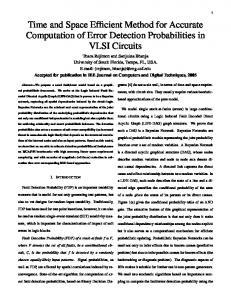
from the given points in this space. This algorithm is quite complex and solution can be found in [18]. It should be noted, that all methods above do have one significant drawback as values are taken in a squared value. This results to an artifact that small values do not have relevant influence to the final entity as the high values. Some methods are trying to overcome this by setting weights to each measured data [3]. It should be noted that the TLSE was originally derived by Pearson [16](1901). Deep comprehensive analysis can be found in [8][13][21][22]. Differences between the LSE a TLSE methods approaches are significant, see Fig.1.

y

y

x

x

I. INTRODUCTION Wide range of applications is based on approximation of acquired data and the LSE minimization is used, known also as a linear or polynomial regression. The regression methods have been heavily explored in signal processing and geometrical problems or with statistically oriented problems. They are used across many engineering fields dealing with acquired data processing. Several studies have been published and they can be classified as follows:  “standard” Least Square Error (LSE) methods fitting data to a function 𝑦 = 𝑓(𝒙) , where 𝒙 is an independent variable and 𝑦 is a measured or given value,  “orthogonal” Total Least Square Error (TLSE) fitting data to a function 𝐹(𝒙) = 0 , i.e. fitting data to some 𝑑 − 1dimensional entity in this 𝑑-dimensional space, e.g. a line in the 𝐸 2 space or a plane in the 𝐸 3 space [1][6][8][21][22],  “orthogonally Mapping” Total Least Square Error (MTLSE) methods for fitting data to a given entity in a subspace of the given space. However, this problem is much more complicated. As an example, we can consider data given in and we need to find an optimal line in 𝐸 𝑑 , i.e. one dimensional entity, in this 𝑑-dimensional space fitting optimally the given data. Typical problem: Find a line in the 𝐸 𝑑 space that has the minimum orthogonal distance Research was supported by the and National Science Foundations (GACR) project No. 17-05534S.

Fig. 1.a: Least Square Error

Fig.1.b: Total Least Square Error

In the vast majority the Least Square Error (LSE) methods measuring vertical distances are used. This approach is acceptable in the case of explicit functional dependences 𝑓(𝑥, 𝑦) = ℎ, resp. 𝑓(𝑥, 𝑦, 𝑧) = ℎ. However, it should be noted that a user should keep in a mind, that smaller differences than 1.0, will have significantly smaller weight than higher differences than 1.0 as the differences are taken in a square resulting to dependences in scaling of data approximated, i.e. the result will depend on physical units used, etc. The main advantage of the LSE method is that it is simple for fitting polynomial curves and it is easy to implement. The standard LSE method leads to over determined system of linear equations. This approach is also known as polynomial regression. Let us consider a data set Ω = {〈𝑥𝑖 , 𝑦𝑖 , 𝑓𝑖 〉}𝑛𝑖=1 , i.e. data set containing for 𝑥𝑖 ,𝑦𝑖 and measured functional value 𝑓𝑖 , and we want to find parameters 𝒂 = [𝑎, 𝑏, 𝑐, 𝑑]𝑇 for optimal fitting function, as an example: 𝑓(𝑥, 𝑦, 𝒂) = 𝑎 + 𝑏𝑥 + 𝑐𝑦 + 𝑑𝑥𝑦 Minimizing the vertical squared distance 𝐷, i.e.:

(1)

FedCSIS 2017, IEEE, ISSN 2300-5963

doi 10.15439/978-83-946253-7

𝑛

where 𝒃 = (𝑏1 , … , 𝑏𝑛 ), 𝝃 = (𝜉1 , … , 𝜉𝑚 ) and 𝑚 is a number of parameters, 𝑚 < 𝑛.

2

𝐷 = min ∑(𝑓𝑖 − 𝑓(𝑥𝑖 , 𝑦𝑖 , 𝒂)) = 𝑎,𝑏,𝑐,𝑑

(2)

𝑖=1

𝑛

𝑚𝑖𝑛 ∑(𝑓𝑖 − (𝑎 + 𝑏𝑥𝑖 + 𝑐𝑦𝑖 + 𝑑𝑥𝑖 𝑦𝑖 ))

𝑎,𝑏,𝑐,𝑑

2

𝑖=1

Conditions for an extreme are given as: 𝜕𝑓(𝑥, 𝑦, 𝒂) (3) = [1, 𝑥, 𝑦, 𝑥𝑦]𝑇 𝜕𝒂 Applying this on the expression of 𝐷 we obtain 𝑛 𝜕𝐷 𝜕𝑓(𝑥, 𝑦, 𝒂) ∑(𝑓𝑖 − (𝑎 + 𝑏𝑥𝑖 + 𝑐𝑦𝑖 + 𝑑𝑥𝑖 𝑦𝑖 )) = 0 (4) 𝜕𝒂 𝜕𝒂 𝑖=1 It leads to conditions for 𝒂 = (𝑎, 𝑏, 𝑐, 𝑑) parameteters in the form of a linear system of equations 𝑨𝒙 = 𝒃: 𝑨= 𝑛

𝑛 𝑛

∑

𝑖=1 𝑛

∑

𝑖=1 𝑛

𝑛

𝑛

∑

𝑥𝑖

∑

𝑦𝑖

∑

𝑥𝑖 𝑦𝑖

𝑥𝑖

∑

𝑥𝑖2

∑

𝑥𝑖 𝑦𝑖

∑

𝑥𝑖2 𝑦𝑖

𝑦𝑖

∑

𝑥𝑖 𝑦𝑖

∑

𝑦𝑖2

∑

𝑥𝑖 𝑦𝑖2

∑

𝑥𝑖2 𝑦𝑖

∑

𝑥𝑖 𝑦𝑖2

∑

𝑥𝑖2 𝑦𝑖2

𝑖=1 𝑛 𝑖=1 𝑛 𝑖=1 𝑛

∑ 𝑥𝑦 [ 𝑖=1 𝑖 𝑖 𝑛

𝒃 = [∑

𝑖=1

𝑖=1 𝑛 𝑖=1 𝑛 𝑖=1 𝑛 𝑖=1

𝑖=1 𝑛

𝑛

𝑓𝑖 , ∑

𝑖=1

𝑛

𝑓𝑖 𝑥𝑖 , ∑

𝑖=1

𝑖=1

(5)

𝑖=1 𝑛 𝑖=1

𝑛

𝑓𝑖 𝑦𝑖 , ∑

𝑖=1

]

𝑻

𝑓𝑖 𝑥𝑖 𝑦𝑖 ]

The selection of bilinear form was used to show the LSE method application to a non-linear case, if the case of a linear function, i.e. 𝑓(𝑥, 𝑦, 𝒂) = 𝑎 + 𝑏𝑥 + 𝑐𝑦, the 4th row and column are to be removed. Note that the matrix 𝑨 is symmetric and the function 𝑓(𝒙) might be more complex, in general. Several methods for LSE have been derived [4][5][10], however those methods are sensitive to the vector 𝒂 orientation and not robust in general as a value of ∑𝑛𝑖=1 𝑥𝑖2 𝑦𝑖2 might be too high in comparison with the value 𝑛, which has an influence to robustness of a numerical solution. In addition, the LSE methods are sensitive to a rotation as they measure vertical distances. It should be noted, that rotational and translation invariances are fundamental requirements especially in geometrically oriented applications. The LSE method is usually used for a small size of data and span of a domain is relatively small. However, in some applications the domain span can easily be over several decades, e.g. in the case of Radial Basis Functions (RBF) approximation for GIS applications etc. In this case, the overdetermined system can be difficult to solve. II. NUMERICAL STABILITY Let us explore a simple example, when many points 𝒙𝑖 ∈ 𝐸 2 , i.e. 𝒙𝑖 = (𝑥𝑖 , 𝑦𝑖 ) , are given with relevant associated values 𝑏𝑖 , 𝑖 = 1, … , 𝑛. Expected functional dependency can be expressed (for a simplicity) as 𝑦 = 𝑎1 + 𝑎2 𝑥 + 𝑎3 𝑦. The LSE leads to an overdetermined system of equations 𝑨𝑇 𝑨 𝝃 = 𝑨𝑇 𝒃

If the values 𝑥𝑖 , 𝑦𝑖 over a large span, e.g. 𝑥𝑖 , 𝑦𝑖 ∈ 〈100 , 105 〉, the matrix 𝑨𝑇 𝑨 is extremely ill conditioned. This means that the reliability of a solution depends on the distribution of points in the domain. Situation gets worst when a non-linear polynomial regression is to be used and dimensionality of the domain is higher. As an example, let us consider a simple case, when points form regular orthogonal mesh and values are generated using 𝑅5 distribution scheme (equidistant in a logarithmic scale) as (𝑥𝑖 , 𝑦𝑖 ) ∈ 〈10, 105 〉 × 〈10, 105 〉. It can be easily found using MATLAB that conditional number 𝑐𝑜𝑛𝑑(𝑨𝑇 𝑨) ≅ 1011 . In the following, we will show how the condition number might be decreased significantly using orthogonal basis vectors instead of the orthonormal ones. III.

𝑖=1 𝑛

𝒙 = [𝑎, 𝑏, 𝑐 , 𝑑 ]𝑻

pp.537-541

(6)

PROJECTIVE NOTATION AND GEOMETRY ALGEBRA

The LSE approximation is based on a solution of a linear system of equations, i.e. 𝑨𝒙 = 𝒃. Usually the Euclidean representation is used. However if the projective space representation is used [19] , it is transformed into homogeneous linear system of equations, i.e. 𝑩𝜻 = 𝟎. Rewriting the Eq.(6), we obtain (7) 𝑩𝜻 = 𝟎 where 𝑩 = [−𝑨𝑇 𝒃|𝑨𝑇 𝑨] (8) 𝜻 = (𝜁0 : 𝜁1 , … , 𝜁𝑚 ) 𝜁 and 𝜉𝑖 = 𝑖⁄𝜁 , 𝑖 = 1, … , 𝑚; 𝜁0 is the homogeneous coordinate 0 in the projective representation, matrix 𝑩 size is 𝑚 × (𝑚 + 1). Now, a system of homogeneous linear equations is to me solved. It can be shown that a system of homogeneous linear equations 𝑨𝒙 = 𝟎 is equivalent to the extended cross-product, actually outer-product [19][20]. In general, solutions of the both cases 𝑨𝒙 = 𝟎 and 𝑨𝒙 = 𝒃, i.e. homogeneous and nonhomogeneous system of linear equations, is the same and no division operation is needed as the extended cross-product (outer product) does not require any division operation at all. Applying this we get: (9) 𝜻 = (𝜁0 : 𝜁1 , … , 𝜁𝑚 ) = 𝜷1 ∧ 𝜷2 ∧ … ∧ 𝜷𝑚−1 ∧ 𝜷𝑚 where (10) 𝜷𝑖 = [−𝑏𝑖0 : 𝑏𝑖1 , … , 𝑏𝑖𝑚 ]𝑇 𝑖 = 1, … , 𝑚 The extended cross-product can be rewritten using determinant of (𝑚 + 1) × (𝑚 + 1) as 𝒆0 𝒆1 𝒆2 ⋯ 𝒆𝑚 −𝑏10 𝑏11 𝑏12 ⋯ 𝑏1𝑚 (11) 𝜻 = det [ ⋮ ⋮ ⋮ ⋱ ⋮ ] −𝑏𝑚0 𝑏𝑚1 𝑏𝑚2 ⋯ 𝑏𝑚𝑚 where 𝒆0 are orthonormal basis vectors in the 𝑚-dimensional space. As a determinant is a multilinear, we can multiply any 𝑗 column by a value 𝑞𝑗 ≠ 0

FedCSIS 2017, IEEE, ISSN 2300-5963

𝜻′ =

𝒆′0 −𝑏 ′ det [ 10

⋮ ′ −𝑏𝑚0

where

𝒆1′ ′ 𝑏11

⋮ ′ −𝑏𝑚1

𝒆′2 ′ 𝑏12

⋮ ′ −𝑏𝑚2

𝒆𝑗 𝑞𝑗

⋯ ⋯ ⋱ ⋯

doi 10.15439/978-83-946253-7

𝒆′𝑚 ′ 𝑏1𝑚

⋮ ′ −𝑏𝑚𝑚

]

(12)

pp.537-541

Using the approach presented above, the conditional number 𝑇 𝑨) ≅ 2. 106 . ̅̅̅̅̅̅ was decreased significantly to 𝑐𝑜𝑛𝑑(𝑨

𝑏∗𝑗 (13) 𝑞𝑗 where 𝒆𝑗′ are orthogonal basis vectors in the 𝑚-dimensional space. 𝒆𝑗′ =

′ 𝑏∗𝑗 =

From the geometrical point of view, it is actually a “temporary” scaling on each axis including the units. Of course, a question remains – how to select the 𝑞𝑗 value. The 𝑞𝑗 is to be selected as 𝑞𝑗 = max {|𝑏𝑖𝑗 |} 𝑖=1,…,𝑚

(14)

where 𝑗 = 1, … , 𝑚. Note that the matrix 𝑩 is indexed as (0, … , 𝑚) × (0, … , 𝑚).

Fig.3: Conditionality of the modified matrix depending on number of data set size, i.e. number of points

Comparing the condition numbers of the original and modified matrices, we can see significant improvement of matrix conditionality as 10

Applying this approach, we get a modified system ′ ) (15) 𝜻′ = (𝜁0′ : 𝜁1′ , … , 𝜁𝑚 = 𝜷1′ ∧ 𝜷′2 ∧ … ∧ 𝜷′𝑚−1 ∧ 𝜷′𝑚 where ′ ′ ′ 𝑇 ] (16) 𝜷′𝑖 = [−𝑏𝑖0 : 𝑏𝑖1 , … , 𝑏𝑖𝑚 ′ 𝑇 𝑨], i.e. ̅̅̅̅̅̅ ̅ ´ = [−𝑨𝑇 𝒃|𝑨 where 𝜷𝑖 are coefficients of the matrix 𝑩 modified matrix 𝑩 as described above, for the orthogonal (not orthonormal) vector basis.

𝑇 6.10 (19) 𝜐 = 𝑐𝑜𝑛𝑑(𝑨 𝑨)⁄ ≅ = 3.104 𝑇 ̅̅̅̅̅̅ 𝑐𝑜𝑛𝑑(𝑨 𝑨) 2.106 In the case of a little bit more complex function defined by Eq.(1), i.e. 𝑓(𝑥, 𝑦) = 𝑎 + 𝑏𝑥 + 𝑐𝑦 + 𝑑𝑥𝑦 we obtain

The approximated 𝑓(𝑥, 𝑦) value is computed as 𝑓(𝑥, 𝑦) = 𝑎𝑞1 + 𝑏𝑞2 𝑥 + 𝑐𝑞3 𝑦 in the case of 𝑓(𝑥, 𝑦) = 𝑎 + 𝑏𝑥 + 𝑐𝑦, or

(17)

(18) 𝑓(𝑥, 𝑦) = 𝑎𝑞1 + 𝑏𝑞2 𝑥 + 𝑐𝑞3 𝑦 + 𝑑𝑞4 𝑥𝑦 in the case 𝑓(𝑥, 𝑦) = 𝑎 + 𝑏𝑥 + 𝑐𝑦 + 𝑑𝑥𝑦 and similarly for the general case of a regression function 𝑦 = 𝑓(𝒙, 𝒂). The above presented modification is simple. However, what is the influence of this operation?

Fig.4: Conditionality of the original matrix depending on number of data set size, i.e. number of points

IV. MATRIX CONDITIONALITY Let us consider a recent simple example again, when points are generated from (𝑥𝑖 , 𝑦𝑖 ) ∈ 〈10, 105 〉 × 〈10, 105 〉. It can be found that conditional number 𝑐𝑜𝑛𝑑(𝑨𝑇 𝑨) ≅ 6. 1010 using MATLAB, Fig.2, if 𝑓(𝑥, 𝑦) = 𝑎 + 𝑏𝑥 + 𝑐𝑦 is used for the LSE.

Fig.5: Conditionality of the modified matrix depending on number of data set size, i.e. number of points

In this case of the LSE defined by Eq.(1) the conditionality improvement is even higher, as 20

Fig.2: Conditionality histogram of the original matrix depending on number of data set size, i.e. number of points

𝑇 6.10 (20) 𝜐 = 𝑐𝑜𝑛𝑑(𝑨 𝑨)⁄ ≅ = 109 𝑇 ̅̅̅̅̅̅ 𝑐𝑜𝑛𝑑(𝑨 𝑨) 6.1011 It means that better numerical stability is obtained by a simple operation. All graphs clearly shows also dependency on a number of points used for the experiments (horizontal axis).

FedCSIS 2017, IEEE, ISSN 2300-5963

doi 10.15439/978-83-946253-7

The geometric algebra brings also an interesting view on problems with numerical solutions. Let us consider vectors ̂ 𝜷𝑖 with coordinates of points, i.e. ̂ 𝑖 = [𝑏𝑖1 , … , 𝑏𝑖𝑚 ]𝑇 𝑖 = 1, … , 𝑚 (21) 𝜷 ̂𝑖 ∧ 𝜷 ̂𝑗 = 𝜸 ̂𝑖𝑗 defines a bivector, which is an oriented Then 𝜷 ̂𝑖𝑗 ‖ surface, given by two vectors in 𝑚-dimensional space and ‖𝜸 gives the area represented by the bivector ̂𝜸𝑖𝑗 . So, the proposed approach of introducing orthogonal basis functions instead of the orthonormal ones, enable us to “eliminate” influence of “small” bivectors in the original LSE computation and increase precision of numerical computation. Of course, if the regression is to be applied, the influence of the 𝑞𝑗 values must be applied. By the presented approach we actually got values 𝜁𝑖′ using the orthogonal basis vectors instead of orthonormal. It means, that the estimated value by a regression, using recent simple example, is (22) 𝑓(𝑥, 𝑦) = 𝑞1 𝑎1 + 𝑞2 𝑎2 𝑥 + 𝑞3 𝑎3 𝑦 In the case of the least square approximation, we want to minimize using a polynomial of degree 𝑛. min ‖𝑓(𝑥) − 𝑃𝑛 (𝑥)‖ 𝑘

(23)

𝑃𝑛 (𝑥) = ∑ 𝑎𝑖 𝑥 𝑖 𝑖=0

The 𝐿2 norme of a function 𝑓(𝑥) an an interval 〈𝑎, 𝑏〉 is defined 2

𝑏

‖𝑓(𝑥)‖ = √(∫ 𝑓(𝑥)𝑑𝑥 )

𝑏

𝑏

∑ 𝑎𝑖 ∫ 𝑥 𝑖+𝑘 𝑑𝑥 = ∫ 𝑥 𝑘 𝑓(𝑥)𝑑𝑥 𝑖=0

𝑎

(29)

𝑎

where 𝑘 = 1, … , 𝑛. It means that the LSE problem is the polynomial (what has been expected) 𝑘

𝑃𝑛 (𝑥) = ∑ 𝑎𝑖 𝑥 𝑖

(30)

𝑖=0

However, there is a direct connection with well known Hilbert’s matrix. It can be shown that elements of the Hilbert’s matrix (𝐻𝑛+1 (𝑎, 𝑏))𝑖,𝑘 of the size (𝑛 + 1) × (𝑛 + 1) are equivalent to 𝑏 1 (31) (𝐻𝑛+1 (𝑎, 𝑏))𝑖,𝑘 = ∫ 𝑥 𝑖+𝑘 𝑑𝑥 = 1+𝑖+𝑘 𝑎 If interval 〈𝑎, 𝑏〉 = 〈0,1〉 is used, standard Hilbert’s matrix 𝑯𝑛 (0,1) is obtained, which is extremely ill-conditioned. VI. HILBERT’S MATRIX CONDITIONALITY

V. LEAST SQUARE METHOD WITH POLYNOMIALS

𝑃𝑛 (𝑥)

pp.537-541 𝑛

(24)

We should answer a question, how the conditional number of the Hilbert’s matrix can be improved if orthogonal basis is used instead of orthonormal one as an experimental test. A simple experiment can prove that the proposed method does not practically change the conditionality of the Hilbert’s matrix 𝑯𝑛 (0,1). However, as the LSE approximation is to be used for large span of data, it is reasonable to consider a general case and explore conditionality of the 𝑯𝑛 (𝑎, 𝑏) matrix, e.g. 𝑯5 (0, 𝑏), for demonstration.

𝑎

Minimizing square of the distance of a function of 𝑘 + 1 parameters 𝜑(𝒂) = 𝜑(𝑎0 , … , 𝑎𝑛 ) and using “per-partes” rule, we obtain 𝑏

𝜑(𝒂) = ∫ [𝑓(𝑥) − 𝑃𝑛 (𝑥)]2 𝑑𝑥 𝑎

𝑏

=∫

[𝑓(𝑥)]2

𝑎

𝑛

𝑏

𝑑𝑥 − 2 ∑ 𝑎𝑖 ∫ 𝑥𝑖 𝑓(𝑥)𝑑𝑥 𝑖=0 𝑛 𝑛

𝑎

(25) Fig.6: Conditionality of the 𝑯5 (0, 𝑏) for different values of 𝑏 using MATLAB (numerical problems can be seen for 𝑏 > 650)

𝑏

+ ∑ ∑ 𝑎𝑖 𝑎𝑗 ∫ 𝑥 𝑖+𝑗 𝑑𝑥 𝑎

𝑖=0 𝑗=0

For a minimum a vector condition 𝜕𝜑(𝒂) =𝟎 𝜕𝒂 must be valid. It leads to conditions 𝑛 𝑏 𝑏 𝜕𝜑(𝒂) 𝑘 = 0 − 2 ∫ 𝑥 𝑓(𝑥)𝑑𝑥 + ∑ 𝑎𝑖 ∫ 𝑥 𝑖+𝑘 𝑑𝑥 𝜕𝑎𝑘 𝑎 𝑎 𝑖=0

𝑛

𝑏

+ ∑ 𝑎𝑗 ∫ 𝑥

𝑗+𝑘

(26)

(27)

𝑑𝑥

Fig.7: Conditionality of the 𝑯5 (0, 𝑏) for different values of 𝑏 using logarithmic scaling for vertical axis

𝑎

𝑖=0

and by simple algebraic manipulations we obtain: 𝑏

𝑛

𝑘

𝑏

2 [− ∫ 𝑥 𝑓(𝑥)𝑑𝑥 + ∑ 𝑎𝑖 ∫ 𝑥 𝑎

and therefore

𝑖=0

𝑎

𝑖+𝑘

𝑑𝑥 ] = 0

(28)

It can be seen, that 𝑐𝑜𝑛𝑑(𝑯5 (0,800)) = 6. 1023 . If the 14 ̅̅̅̅̅̅̅̅̅̅̅̅̅̅ proposed approach is applied 𝑐𝑜𝑛𝑑(𝑯 5 (0,800)) = 2,5. 10 for the modified matrix, Fig.8 - Fig.9.

FedCSIS 2017, IEEE, ISSN 2300-5963

doi 10.15439/978-83-946253-7

pp.537-541

VII. CONCLUSIONS The proposed method of application orthogonal vector basis instead of the orthonormal one decreases conditional number of a matrix used in the least square method. This approach increases robustness of a numerical solution especially when domain data range is high. It can be used also for solving systems of linear equations in general, e.g. if radial basis function interpolation or approximation is used. ACKNOWLEDGMENT Fig.8: Conditionality of the modified 𝑯5 (0, 𝑏)

The author would like to thank to colleagues at the University of West Bohemia in Plzen for fruitful discussions and to anonymous reviewers for their comments and hints, which helped to improve the manuscript significantly. Special thanks belong to Zuzana Majdišová and Michal Šmolík for independent experiments, images and generation in MATLAB. REFERENCES

Fig.9: Conditionality of the modified 𝑯5 (0, 𝑏) using logarithmic scaling for vertical axis

It means that the conditionality improvement 𝑐𝑜𝑛𝑑(𝑯5 (0,800)) 6.1023 𝜐= ≅ ≈ 109 (32) ̅̅̅̅̅̅̅̅̅̅̅̅̅̅ 2,5.1014 𝑐𝑜𝑛𝑑(𝑯 5 (0,800)) This is a similar ratio as for the simple recent examples. A change of the size of bivectors ‖𝜷𝑖 ∧ 𝜷𝑗 ‖ can be used as a practical result using RBF approximation, which changes from the interval 〈𝑒𝑝𝑠, 1010 〉 to 〈𝑒𝑝𝑠, 8. 102 〉, which significantly increases robustness of the RBF approximation, Fig.10.

Fig.10: Bivector histogram sizes for original LSE matrix and modified one

The proposed approach has been used for St.Helen’s volcano approximation by 10 000 points instead of 6 743 176 original points, see Fig.11.

Fig.11: LSE approximation error with RBF approximation of St.Helen’s (image generated in MATLAB by Michal Smolik)

[1] Abatzoglou,T., Mendel,J. 1987. Constrained total least squares, IEEE Conf. Acoust., Speech, Signal Process. (ICASSP’87), Vol. 12, 1485–1488. [2] Alciatore,D., Miranda,R. 1995. The best least-square line fit, Graphics Gems V (Ed.Paeth,A.W.), 91-97, Academic Press. [3] Amiri-Simkooei,A.R.,Jazaeri,S. 2012.Weighted total least squares formulated by standard least squares theory,J.Geodetic Sci.,2(2):113-124. [4] Charpa,S., Canale,R. 1988. Numerical methods for Engineers, McGrawHill. [5] Chatfield,C. 1970. Statistics for technology, Penguin Book. [6] de Groen,P. 1996 An introduction to total least squares, Nieuw Archief voor Wiskunde,Vierde serie, deel 14, 237–253 [7] DeGroat,R.D., Dowling,E.M. 1993 The data least squares problem and channel equalization. IEEE Trans. Signal Processing, Vol. 41(1), 407–411. [8] Golub,G.H., Van Loan,C.F. 1980. An analysis of the total least squares problem. SIAM J. on Numer. Anal., 17, 883–893. [9] Jo,S., Kim,S.W. 2005. Consistent normalized least mean square filtering with noisy data matrix. IEEE Trans. Signal Proc.,Vol. 53(6), 2112–2123. [10] Kryszig,V. 1983. Advanced engineering mathematics, John Wiley & Sons. [11] Lee,S.L. 1994. A note on the total least square fit to coplanar points, Tech.Rep. ORNL-TM-12852, Oak Ridge National Laboratory. [12] Levy,D., 2010. Introduction to Numerical Analysis, Univ.of Maryland [13] Nievergelt,Y. 1994. Total least squares: State of the Art regression in numerical mathematics, SIAM Review, Vol.36, 258-264 [14] Nixon,M.S., Aguado,A.S. 2012. Feature extraction & image processing for computer vision, Academic Press. [15] Markowsky,I., VanHueffel,S., 2007. Overview of total least square methods, Signal Processing, 87 (10), 2283-2302. [16] Pearson,K., 1901. On line and planes of closest fit to system of points in space, Phil.Mag., Vol.2, 559-572 [17] Skala,V., 2016.Total Least Square Error Computation in E2: A New Simple, Fast and Robust Algorithm, CGI 2016 Proc., ACM, pp.1-4, Greece [18] Skala,V., 2016. A new formulation for total Least Square Error method in d-dimensional space with mapping to a parametric line, ICNAAM 2015, AIP Conf. Proc.1738, pp.480106-1 - 480106-4, Greece [19] Skala,V., 2017. Least Square Error method approximation and extended cross product using projective representation, ICNAAM 2016 conf., to appear in ICNAAM 2016 proceedings, AIP Press [20] Skala,V., 2008. Barycentric Coordinates Computation in Homogeneous Coordinates, Computers & Graphics, Elsevier, , Vol.32, No.1, pp.120-127 [21] Van Huffel,S., Vandewalle,J 1991. The total least squares problems: computational aspects and analysis. SIAM Publications, Philadelphia PA. [22] van Huffel,S., Lemmerling,P. 2002. Total least squares and errors-invariables modeling: Analysis, algorithms and applications. Dordrecht, The Netherlands: Kluwer Academic Publishers [23] Perpendicular regression of a line (download 2015-12-20) http://www.mathpages.com/home/kmath110.htm [24] Skala,V., 2017. RBF Interpolation with CSRBF of Large Data Sets, ICCS 2017, Procedia Computer Science, Vol.108, pp. 2433-2437, Elsevier [25] Skala,V., 2017. High Dimensional and Large Span Data Least Square Error: Numerical Stability and Conditionality, accepted to ICPAM 2017