Entropy 2013, 15, 3746-3761; doi:10.3390/e15093746 OPEN ACCESS
entropy ISSN 1099-4300 www.mdpi.com/journal/entropy Article
Combination Synchronization of Three Identical or Different Nonlinear Complex Hyperchaotic Systems Xiaobing Zhou *, Murong Jiang and Yaqun Huang School of Information Science and Engineering, Yunnan University, Kunming 650091, China * Author to whom correspondence should be addressed; E-Mail:
[email protected]. Received: 5 August 2013; in revised form: 3 September 2013 / Accepted: 4 September 2013 / Published: 10 September 2013
Abstract: In this paper, we investigate the combination synchronization of three nonlinear complex hyperchaotic systems: the complex hyperchaotic Lorenz system, the complex hyperchaotic Chen system and the complex hyperchaotic L¨u system. Based on the Lyapunov stability theory, corresponding controllers to achieve combination synchronization among three identical or different nonlinear complex hyperchaotic systems are derived, respectively. Numerical simulations are presented to demonstrate the validity and feasibility of the theoretical analysis. Keywords: combination synchronization; Lyapunov stability theory; complex hyperchaotic Lorenz system; complex hyperchaotic Chen system; complex hyperchaotic L¨u system
1. Introduction Since Fowler et al. [1], introduced a complex Lorenz model to generalize the real Lorenz model in 1982, complex chaotic and hyperchaotic systems have attracted increasing attention, due to the fact that systems with complex variables can be used to describe the physics of a detuned laser, rotating fluids, disk dynamos, electronic circuits and particle beam dynamics in high energy accelerators [2]. When applying complex systems in communications, the complex variables will double the number of variables and can increase the content and security of the transmitted information. Many complex chaotic and hyperchaotic systems have been proposed ever since the 1980s. In [3], the authors studied the chaotic unstable limit cycles of complex Van der Pol oscillators. The rich dynamics behaviors of the complex Chen and complex L¨u systems were investigated in [4]. By adding state feedback controllers to
Entropy 2013, 15
3747
their complex chaotic systems, complex hyperchaotic Chen, Lorenz and L¨u systems were introduced and studied in [5–7], respectively. The authors [8] constructed a complex nonlinear hyperchaotic system by adding a cross-product nonlinear term to the complex Lorenz system. A complex modified hyperchaotic L¨u system [9] was proposed by introducing complex variables to its real counterpart. In 1990 [10], Pecora and Carroll proposed the drive-response concept for constructing the synchronization of coupled chaotic systems. Over the last two decades, synchronization in chaotic systems has been extensively investigated, due to its potential applications in various fields, such as chemical reactions, biological systems and secure communication. Mahmoud et al. [11] designed an adaptive control scheme to study the complete synchronization of chaotic complex nonlinear systems with uncertain parameters. The authors achieved phase synchronization and antiphase synchronization of two identical hyperchaotic complex nonlinear systems via an active control technique in [12]. Based on passive theory, the authors studied the projective synchronization of hyperchaotic complex nonlinear systems and its application in secure communications [13]. Liu et al. [14] investigated the modified function projective synchronization of general chaotic complex systems described by a unified mathematical expression. The aforementioned synchronization schemes are based on the usual drive-response synchronization mode, which has one drive system and one response system. Recently, Luo [15] proposed a combination synchronization scheme, which has two drive systems and one response system. This synchronization scheme has advantages over the usual drive-response synchronization, such as being able to provide greater security in secure communication. In secure communication, the transmitted signals can be split into several parts, each part loaded in different drive systems, or can divide time into different intervals, the signals in different intervals being loaded in different drive systems. Thus, the transmitted signals can have stronger anti-attack ability and anti-translated capability than those transmitted by the usual transmission model. Motivated by the above discussions, this paper aims to study the combination synchronization of three identical or different nonlinear complex hyperchaotic systems. The rest of this paper is organized as follows. Section 2 introduces the scheme of combination synchronization. In Section 3 and Section 4, we investigate combination synchronization among three identical and different complex nonlinear hyperchaotic systems, respectively. Finally, conclusions are given in Section 5. 2. The Scheme of Combination Synchronization Suppose that there are three nonlinear dynamical systems, two drive systems and one response system. The drive systems are given by: x˙ = f (x), (1) and y˙ = g(y).
(2)
z˙ = h(z) + U (x, y, z),
(3)
The response system is described by:
Entropy 2013, 15
3748
where x = (x1 , x2 , ..., xn )T , y = (y1 , y2 , ..., yn )T , z = (z1 , z2 , ..., zn )T are the state vectors of systems (1), (2) and (3), respectively, f (·), g(·), h(·) : Rn → Rn are three continuous vector functions and U (·) : Rn × Rn × Rn → Rn is a controller vector, which will be designed. Definition 1 [15]. For drive systems (1) and (2) and response system (3), they are said to be in combination synchronization if there exists three constant matrices, A, B, C ∈ Rn and C ̸= 0, such that: lim ∥ Ax + By − Cz ∥= 0, (4) t→+∞
where ∥ · ∥ represents the matrix norm. 3. Combination Synchronization among Identical Nonlinear Complex Hyperchaotic Systems In this section, we take the complex hyperchaotic Lorenz system [6] as an example to investigate the combination synchronization among three identical systems. The first drive system is given by: x˙ 11 = α(x21 − x11 ) + x41 , x˙ 21 = γx11 − x21 − x11 x31 , 1 (5) x˙ 31 = (¯ x11 x21 + x11 x¯21 ) − βx31 + x41 , 2 x˙ 41 = 1 (¯ x11 x21 + x11 x¯21 ) − σx41 , 2 and the second drive system is described as follows: x˙ 12 = α(x22 − x12 ) + x42 , x˙ 22 = γx12 − x22 − x12 x32 , 1 x˙ 32 = (¯ x12 x22 + x12 x¯22 ) − βx32 + x42 , 2 x˙ 42 = 1 (¯ x12 x22 + x12 x¯22 ) − σx42 . 2 The response system takes the following form: x˙ 13 = α(x23 − x13 ) + x43 + U1 + iU2 , x˙ 23 = γx13 − x23 − x13 x33 + U3 + iU4 , 1 x13 x23 + x13 x¯2 ) − βx33 + x43 + U5 , x˙ 33 = (¯ 2 x˙ 43 = 1 (¯ x13 x23 + x13 x¯23 ) − σx43 + U6 , 2
(6)
(7)
where α, β, γ and σ are positive parameters, x11 = u1 + iu2 , x21 = u3 + iu4 , x12 = v1 + iv2 , x22 = √ v3 +iv4 , x13 = w1 +iw2 , x23 = w3 +iw4 are complex variables and i = −1; ui , vi , wi (i = 1, 2, 3, 4), x31 = u5 , x41 = u6 , x32 = v5 , x42 = v6 , x33 = w5 , x43 = w6 are real variables. The overbar represents a complex conjugate function. U1 , U2 , U3 , U4 , U5 and U6 are real controllers to be determined. For the convenience of our discussions, we assume A = diag(l1 , l2 , l3 , l4 ), B = diag(m1 , m2 , m3 , m4 ), C = diag(k1 , k2 , k3 , k4 ) in our synchronization scheme.
Entropy 2013, 15
3749
We define error states between systems (5), (6) and (7) as: e1 + ie2 = k1 x13 − l1 x11 − m1 x12 , e3 + ie4 = k2 x23 − l2 x21 − m2 x22 , such that:
e5 = k3 x33 − l3 x31 − m3 x32 ,
(8)
e6 = k4 x43 − l4 x41 − m4 x42 ,
lim ∥ k1 x13 − l1 x11 − m1 x12 ∥= 0, t→∞ lim ∥ k2 x23 − l2 x21 − m2 x22 ∥= 0, t→∞
lim ∥ k3 x33 − l3 x31 − m3 x32 ∥= 0, t→∞ lim ∥ k4 x43 − l4 x41 − m4 x42 ∥= 0.
(9)
t→∞
Thus, we have the following error dynamical system: e˙ 1 + ie˙ 2 = k1 x˙ 13 − l1 x˙ 11 − m1 x˙ 12 , e˙ 3 + ie˙ 4 = k2 x˙ 23 − l2 x˙ 21 − m2 x˙ 22 , e˙ 5 = k3 x˙ 33 − l3 x˙ 31 − m3 x˙ 32 , e˙ = k x˙ − l x˙ − m x˙ . 6
4 43
4 41
(10)
4 42
Substituting Equations (5)–(7) in Equation (10) and separating the real and imaginary parts yields: e˙ 1 = k1 [α(w3 − w1 ) + w6 ] − l1 [α(u3 − u1 ) + u6 ] − m1 [α(v3 − v1 ) + v6 ] + k1 U1 , e˙ 2 = k1 α(w4 − w2 ) − l1 α(u4 − u2 ) − m1 α(v4 − v2 ) + k1 U2 , e˙ = k2 (γw1 − w3 − w1 w5 ) − l2 (γu1 − u3 − u1 u5 ) − m2 (γv1 − v3 − v1 v5 ) + k2 U3 , 3 (11) e˙ 4 = k2 (γw2 − w4 − w2 w5 ) − l2 (γu2 − u4 − u2 u5 ) − m2 (γv2 − v4 − v2 v5 ) + k2 U4 , e˙ 5 = k3 (w1 w3 + w2 w4 − βw5 + w6 ) − l3 (u1 u3 + u2 u4 − βu5 + u6 ) − m3 (v1 v3 + v2 v4 − βv5 + v6 ) + k3 U5 , e˙ 6 = k4 (w1 w3 + w2 w4 − σw6 ) − l4 (u1 u3 + u2 u4 − σu6 ) − m4 (v1 v3 + v2 v4 − σv6 ) + k4 U6 . Then, we obtain the following results.
Entropy 2013, 15
3750
Theorem 1. If the controllers are chosen as follows:
1 U1 = − {(k1 w1 − l1 u1 − m1 v1 ) + [k1 α(w3 − w1 ) + k1 w6 − l1 α(u3 − u1 ) − l1 u6 k1 − m1 α(v3 − v1 ) − m1 v6 ] − α(k1 w2 − l1 u2 − m1 v2 )}, 1 U = − {(k1 w2 − l1 u2 − m1 v2 ) + [k1 α(w4 − w2 ) − l1 α(u4 − u2 ) − m1 α(v4 − v2 )] 2 k1 + α(k1 w1 − l1 u1 − m1 v1 ) − γ(k2 w3 − l2 u3 − m2 v3 )}, 1 U3 = − {(k2 w3 − l2 u3 − m2 v3 ) + [k2 (γw1 − w3 − w1 w5 ) − l2 (γu1 − u3 − u1 u5 ) k2 − m2 (γv1 − v3 − v1 v5 )] + γ(k1 w2 − l1 u2 − m1 v2 ) − β(k2 w4 − l2 u4 − m2 v4 )}, 1 U4 = − {(k2 w4 − l2 u4 − m2 v4 ) + [k2 (γw2 − w4 − w2 w5 ) − l2 (γu2 − u4 − u2 u5 ) k2 − m2 (γv2 − v4 − v2 v5 )] + β(k2 w3 − l2 u3 − m2 v3 ) − σ(k3 w5 − l3 u5 − m3 v5 )}, 1 U5 = − {(k3 w5 − l3 u5 − m3 v5 ) + [k3 (w1 w3 + w2 w4 − βw5 + w6 ) − l3 (u1 u3 + u2 u4 − βu5 + u6 ) k3 − m3 (v1 v3 + v2 v4 − βv5 + v6 )] + σ(k2 w4 − l2 u4 − m2 v4 ) − α(k4 w6 − l4 u6 − m4 v6 )}, 1 U {(k4 w6 − l4 u6 − m4 v6 ) + [k4 (w1 w3 + w2 w4 − σw6 ) − l4 (u1 u3 + u2 u4 − σu6 ) 6 =− k 4 − m4 (v1 v3 + v2 v4 − σv6 )] + α(k3 w5 − l3 u5 − m3 v5 )}, (12) then driven systems (5) and (6) will achieve combination synchronization with response system (7). Proof. Construct the following Lyapunov function: 1 V = (e21 + e22 + e23 + e24 + e25 + e26 ). 2 Taking the time derivative of V along the trajectory of error dynamical system (11) yields:
(13)
V˙ =e1 e˙ 1 + e2 e˙ 2 + e3 e˙ 3 + e4 e˙ 4 + e5 e˙ 5 + e6 e˙ 6 =e1 {k1 [α(w3 − w1 ) + w6 ] − l1 [α(u3 − u1 ) + u6 ] − m1 [α(v3 − v1 ) + v6 ] + k1 U1 } + e2 [k1 α(w4 − w2 ) − l1 α(u4 − u2 ) − m1 α(v4 − v2 ) + k1 U2 ] + e3 [k2 (γw1 − w3 − w1 w5 ) − l2 (γu1 − u3 − u1 u5 ) − m2 (γv1 − v3 − v1 v5 ) + k2 U3 ] + e4 [k2 (γw2 − w4 − w2 w5 ) − l2 (γu2 − u4 − u2 u5 ) − m2 (γv2 − v4 − v2 v5 ) + k2 U4 ] + e5 [k3 (w1 w3 + w2 w4 − βw5 + w6 ) − l3 (u1 u3 + u2 u4 − βu5 + u6 ) − m3 (v1 v3 + v2 v4 − βv5 + v6 ) + k3 U5 ] + e6 [k4 (w1 w3 + w2 w4 − σw6 ) − l4 (u1 u3 + u2 u4 − σu6 ) − m4 (v1 v3 + v2 v4 − σv6 ) + k4 U6 ]. (14)
Entropy 2013, 15
3751
Substituting Equation (12) into Equation (14), then: V˙ =e1 {k1 [α(w3 − w1 ) + w6 ] − l1 [α(u3 − u1 ) + u6 ] − m1 [α(v3 − v1 ) + v6 ] − [k1 w1 − l1 u1 − m1 v1 + k1 α(w3 − w1 ) + k1 w6 − l1 α(u3 − u1 ) − l1 u6 − m1 α(v3 − v1 ) − m1 v6 − α(k1 w2 − l1 u2 − m1 v2 )]} + e2 {k1 α(w4 − w2 ) − l1 α(u4 − u2 ) − m1 α(v4 − v2 ) − [k1 w2 − l1 u2 − m1 v2 + k1 α(w4 − w2 ) − l1 α(u4 − u2 ) − m1 α(v4 − v2 ) + α(k1 w1 − l1 u1 − m1 v1 ) − γ(k2 w3 − l2 u3 − m2 v3 )]} + e3 {k2 (γw1 − w3 − w1 w5 ) − l2 (γu1 − u3 − u1 u5 ) − m2 (γv1 − v3 − v1 v5 ) − [k2 w3 − l2 u3 − m2 v3 + k2 (γw1 − w3 − w1 w5 ) − l2 (γu1 − u3 − u1 u5 ) − m2 (γv1 − v3 − v1 v5 ) + γ(k1 w2 − l1 u2 − m1 v2 ) − β(k2 w4 − l2 u4 − m2 v4 )]} + e4 {k2 (γw2 − w4 − w2 w5 ) − l2 (γu2 − u4 − u2 u5 ) − m2 (γv2 − v4 − v2 v5 ) − [k2 w4 − l2 u4 − m2 v4 + k2 (γw2 − w4 − w2 w5 ) − l2 (γu2 − u4 − u2 u5 ) − m2 (γv2 − v4 − v2 v5 ) + β(k2 w3 − l2 u3 − m2 v3 ) − σ(k3 w5 − l3 u5 − m3 v5 )]} + e5 {k3 (w1 w3 + w2 w4 − βw5 + w6 ) − l3 (u1 u3 + u2 u4 − βu5 + u6 ) − m3 (v1 v3 + v2 v4 − βv5 + v6 ) − [k3 w5 − l3 u5 − m3 v5 + k3 (w1 w3 + w2 w4 − βw5 + w6 ) − l3 (u1 u3 + u2 u4 − βu5 + u6 ) − m3 (v1 v3 + v2 v4 − βv5 + v6 ) + σ(k2 w4 − l2 u4 − m2 v4 ) − α(k4 w6 − l4 u6 − m4 v6 )]} + e6 {k4 (w1 w3 + w2 w4 − σw6 ) − l4 (u1 u3 + u2 u4 − σu6 ) − m4 (v1 v3 + v2 v4 − σv6 ) − [k4 w6 − l4 u6 − m4 v6 + k4 (w1 w3 + w2 w4 − σw6 ) − l4 (u1 u3 + u2 u4 − σu6 ) − m4 (v1 v3 + v2 v4 − σv6 ) + α(k3 w5 − l3 u5 − m3 v5 )]} =e1 (−e1 + αe2 ) + e2 (−e2 − αe1 + γe3 ) + e3 (−e3 − γe2 + βe4 ) + e4 (−e4 − βe3 + σe5 ) + e5 (−e5 − σe4 + αe6 ) + e6 (−e6 − αe5 ) = − e21 − e22 − e23 − e24 − e25 − e26 . (15) ˙ Since V ≤ 0 as t → ∞, according to the Lyapunov stability theory, we know ei → 0(i = 1, 2, 3, 4, 5, 6), i.e., limt→∞ ∥ e ∥= 0. Therefore, drive systems (5) and (6) will achieve combination synchronization with the response system (7). This completes the proof. The following corollaries can be easily obtained from Theorem 1. Corollary 1. (i) Suppose that l1 = l2 = l3 = l4 = 0 and k1 = k2 = k3 = k4 = 1, and if the controllers are chosen as follows: U1 = − {(w1 − m1 v1 ) + [α(w3 − w1 ) + w6 − m1 α(v3 − v1 ) − m1 v6 ] − α(w2 − m1 v2 )}, U2 = − {(w2 − m1 v2 ) + [α(w4 − w2 ) − m1 α(v4 − v2 )] + α(w1 − m1 v1 ) − γ(w3 − m2 v3 )}}, U = − {(w3 − m2 v3 ) + [(γw1 − w3 − w1 w5 ) − m2 (γv1 − v3 − v1 v5 )] + γ(w2 − m1 v2 ) − β(w4 − m2 v4 )}, 3 U4 = − {(w4 − m2 v4 ) + [(γw2 − w4 − w2 w5 ) − m2 (γv2 − v4 − v2 v5 )] + β(w3 − m2 v3 ) − σ(w5 − m3 v5 )}, U5 = − {(w5 − m3 v5 ) + [(w1 w3 + w2 w4 − βw5 + w6 ) − m3 (v1 v3 + v2 v4 − βv5 + v6 )] + σ(w4 − m2 v4 ) − α(w6 − m4 v6 )}, U6 = − {(w6 − m4 v6 ) + [(w1 w3 + w2 w4 − σw6 ) − m4 (v1 v3 + v2 v4 − σv6 )] + α(w5 − m3 v5 )}, (16) then drive system (6) will achieve projective synchronization with response system (7).
Entropy 2013, 15
3752
(ii) Suppose that m1 = m2 = m3 = m4 = 0 and k1 = k2 = k3 = k4 = 1, and if the controllers are chosen as follows: U1 = − {(w1 − l1 u1 ) + [α(w3 − w1 ) + w6 − l1 α(u3 − u1 ) − l1 u6 ] − α(w2 − l1 u2 )}, U2 = − {(w2 − l1 u2 ) + [α(w4 − w2 ) − l1 α(u4 − u2 )] + α(w1 − l1 u1 ) − γ(w3 − l2 u3 )}, U = − {(w3 − l2 u3 ) + [(γw1 − w3 − w1 w5 ) − l2 (γu1 − u3 − u1 u5 )] + γ(w2 − l1 u2 ) − β(w4 − l2 u4 )}, 3 U4 = − {(w4 − l2 u4 ) + [(γw2 − w4 − w2 w5 ) − l2 (γu2 − u4 − u2 u5 )] + β(w3 − l2 u3 ) − σ(w5 − l3 u5 )}, U5 = − {(w5 − l3 u5 ) + [(w1 w3 + w2 w4 − βw5 + w6 ) − l3 (u1 u3 + u2 u4 − βu5 + u6 )] + σ(w4 − l2 u4 ) − α(w6 − l4 u6 )}, U6 = − {(w6 − l4 u6 ) + [(w1 w3 + w2 w4 − σw6 ) − l4 (u1 u3 + u2 u4 − σu6 )] + α(w5 − l3 u5 )}, (17) then drive system (5) will achieve projective synchronization with response system (7). Corollary 2. Suppose that l1 = l2 = l3 = l4 = 0, m1 = m2 = m3 = m4 = 0 and k1 = k2 = k3 = k4 = 1, and if the controllers are chosen as follows: U1 = −[w1 + α(w3 − w1 ) + w6 − αw2 ], U2 = −[w2 + α(w4 − w2 ) + αw1 − γw3 ], U3 = −(w3 + γw1 − w3 − w1 w5 + γw2 − βw4 ), (18) U = −(w + γw − w − w w + βw − σw ), 4 4 2 4 2 5 3 5 U5 = −(w5 + w1 w3 + w2 w4 − βw5 + w6 + σw4 − αw6 ), U6 = −(w6 + w1 w3 + w2 w4 − σw6 + αw5 ), then system (7) is stabilized to the equilibrium, O(0, 0, 0, 0, 0, 0). Remark 1: The proofs of Corollary 1 and Corollary 2 are similar to those of theorem 1, so we omitted them. In the following, numerical experiments are given to demonstrate our results. The fourth-order Runge-Kutta method is used with a time step size of 0.001. The system parameters are given as α = 8, β = 5, γ = 50 and σ = 15, so that the complex Lorenz system exhibits hyperchaotic behavior. We assume k1 = k2 = k3 = k4 = 1, l1 = l2 = l3 = l4 = 1 and m1 = m2 = m3 = m4 = 1, and the initial states for drive systems (5) and (6) and response system (7) are arbitrarily given by (x11 (0), x21 (0), x31 (0), x41 (0)) = (4 − 0.3i, 2.2 − 0.8i, 4.9, 1.1), (x12 (0), x22 (0), x32 (0), x42 (0)) = (4.4 − 0.6i, 3.3 − 1.4i, 5.3, 1.4) and (x13 (0), x23 (0), x33 (0), x43 (0)) = (4.6 − 1.8i, 1.6 − 1.9i, 2.5, 2), i.e., (u1 (0), u2 (0), u3 (0), u4 (0), u5 (0), u6 (0)) = (4, −0.3, 2.2, −0.8, 4.9, 1.1), (v1 (0), v2 (0), v3 (0), v4 (0), v5 (0), v6 (0)) = (4.4, −0.6, 3.3, −1.4, 5.3, 1.4) and (w1 (0), w2 (0), w3 (0), w4 (0), w5 (0), w6 (0)) = (4.6, −1.8, 1.6, −1.9, 2.5, 2), respectively. The corresponding numerical results are shown in Figures 1 and 2. Figure 1 displays the time response of the combination synchronization errors, e1 , e2 , e3 , e4 , e5 ande6 . The errors converge to zero, which implies that systems (5), (6) and (7) have achieved combination synchronization. Figures 2 depicts the time responses of the states, u1 + v1 versus w1 , u2 + v2 versus w2 , u3 + v3 versus w3 , u4 + v4 versus w4 , u5 + v5 versus w5 and u6 + v6 versus w6 , respectively. Next, suppose that k1 = k2 = k3 = k4 = 1, l1 = l2 = l3 = l4 = 0 and m1 = m2 = m3 = m4 = 0. The time evolution of the states,
Entropy 2013, 15
3753
w1 , w2 , w3 , w4 , w5 , w6 , of system (7) with controller (18) are displayed in Figure 3, which illustrates that system (7) is stabilized to the equilibrium, O(0, 0, 0, 0, 0, 0). Figure 1. Combination synchronization errors, e1 , e2 , e3 , e4 , e5 and e6 , between drive systems (5) and (6) and response system (7). 4
2 0 e2
e1
2 0
−2
−2 0
5
10 t
15
−4
20
4
2
2
1 e4
e3
−4
0 −2 −4
0
5
10 t
15
10 t
15
20
0
5
10 t
15
20
0
5
10 t
15
20
0
−2
20
5
5
0 e6
e5
5
−1
10
0
−5
−5 −10
0
0
5
10 t
15
20
−10
4. Combination Synchronization among Different Nonlinear Complex Hyperchaotic Systems In this section, we investigate the combination synchronization among three different nonlinear complex hyperchaotic systems. The hyperchaotic complex Lorenz system [6] and the hyperchaotic complex Chen system [5], respectively, describe the drive systems: x˙ 1 = α1 (x2 − x1 ) + x4 , x˙ 2 = γ1 x1 − x2 − x1 x3 , 1 (19) x1 x2 + x1 x¯2 ) − β1 x3 + x4 , x˙ 3 = (¯ 2 x˙4 = 1 (¯ x1 x2 + x1 x¯2 ) − σ1 x4 , 2 and
y˙ 1 = α2 (y2 − y1 ), y˙ 2 = (γ2 − α2 )y1 − y1 y3 + γ2 y2 + y4 , 1 y1 y2 + y1 y¯2 ) − β2 y3 + y4 , y˙ 3 = (¯ 2 y˙ 4 = 1 (¯ y1 y2 + y1 y¯2 ) − d2 y4 , 2
(20)
Entropy 2013, 15
3754
Figure 2. Time responses for states ui + vi versus wi , i = 1, 2, ..., 6, respectively. 100
20 u1+v1 w1
50
0
0 −50
u2+v2 w2
−20
0
1
2
3
4
−40
5
0
1
2
t
3
4
5
t
100
50 u3+v3 w3
50
u4+v4 w4
0
0
−50 −100
0
1
2
3
4
−50
5
0
1
2
t 200
4
5
150 u5+v5 w5
150
50
50
0 0
1
2
3
4
u6+v6 w6
100
100
0
3 t
−50
5
0
1
2
t
3
4
5
6
8
10
6
8
10
6
8
10
t
2
4
1 2
6
2
w
w1
Figure 3. Time evolution of the states for system (7).
0 −2
0 −1
0
2
4
6
8
−2
10
0
2
4 t
4
2
2 4
3
1
w
w3
t
0 −1
0 −2
0
2
4
6
8
−4
10
0
2
4 t
2
2
1 6
4
0
w
w5
t
−2 −4
0 −1
0
2
4
6 t
8
10
−2
0
2
4 t
Entropy 2013, 15
3755
and the hyperchaotic complex L¨u system system [7] is the response system given by: z˙1 = ρ3 (z2 − z1 ) + z4 + U1 + iU2 , z˙2 = ν3 z2 − z1 z3 + z4 + U3 + iU4 , 1 z˙3 = (¯ z1 z2 + z1 z¯2 ) − µ3 z3 + U5 , 2 z˙4 = 1 (¯ z1 z2 + z1 z¯2 ) − σ3 z4 + U6 , 2
(21)
where α1 , β1 , γ1 , σ1 , α2 , β2 , γ2 , d2 , ρ3 , ν3 , µ3 and σ3 are positive parameters, x1 = u1 + iu2 , x2 = u3 + iu4 , y1 = v1 + iv2 , y2 = v3 + iv4 , z1 = w1 + iw2 , z2 = w3 + iw4 are complex variables and √ i = −1; ui , vi , wi (i = 1, 2, 3, 4), x3 = u5 , x4 = u6 , y3 = v5 , y4 = v6 , z3 = w5 and z4 = w6 are real variables. The overbar represents the complex conjugate function. U1 , U2 , U3 , U4 , U5 and U6 are real control functions to be determined. For the convenience of the following discussions, we assume A = diag(l1 , l2 , l3 , l4 ), B = diag(m1 , m2 , m3 , m4 ) and C = diag(k1 , k2 , k3 , k4 ) in our synchronization scheme. We define error states between drive systems (19)–(20) and response system (21) as: e1 + ie2 = k1 z1 − l1 x1 − m1 y1 , e3 + ie4 = k2 z2 − l2 x2 − m2 y2 , (22) e = k z − l x − m y , 4 3 3 3 3 3 3 e =k z −l x −m y , 5
such that:
4 4
4 4
4 4
lim ∥ k1 z1 − l1 x1 − m1 y1 ∥= 0, t→∞ lim ∥ k2 z2 − l2 x2 − m2 y2 ∥= 0, t→∞
lim ∥ k3 z3 − l3 x3 − m3 y3 ∥= 0, t→∞ lim ∥ k4 z4 − l4 x4 − m4 y4 ∥= 0.
(23)
t→∞
Separating the real and imagery parts of Equation (22) gets the following: e1 = (k1 w1 − l1 u1 − m1 v1 ), e2 = (k1 w2 − l1 u2 − m1 v2 ), e3 = (k2 w3 − l2 u3 − m2 v3 ), e4 = (k2 w4 − l2 u4 − m2 v4 ), e5 = (k3 w5 − l3 u5 − m3 v5 ), e6 = (k4 w6 − l4 u6 − m4 v6 ).
(24)
Entropy 2013, 15
3756
Thus, we have the following error dynamical system: e˙ 1 = k1 [ρ3 (w3 − w1 ) + w6 ] − l1 [α1 (u3 − u1 ) + u6 ] − m1 α2 (v3 − v1 ) + k1 U1 , e˙ 2 = k1 ρ3 (w4 − w2 ) − l1 α1 (u4 − u2 ) − m1 α2 (v4 − v2 ) + k1 U2 , e˙ 3 = k2 (−w1 w5 + ν3 w3 + w6 ) − l2 (γ1 u1 − u3 − u1 u5 ) − m2 [(γ2 − α2 )v1 − v1 v5 + γ2 v3 + v6 ] + k2 U3 , e˙ 4 = k2 (−w2 w5 + ν3 w4 ) − l2 (γ1 u2 − u4 − u2 u5 ) − m2 [(γ2 − α2 )v2 − v2 v5 + γ2 v4 ] + k2 U4 , e˙ 5 = k3 (w1 w3 + w2 w4 − µ3 w5 ) − l3 (u1 u3 + u2 u4 − β1 u5 + u6 ) − m3 (v1 v3 + v2 v4 − β2 v5 + v6 ) + k3 U5 , e˙ 6 = k4 (w1 w3 + w2 w4 − σ3 w6 ) − l4 (u1 u3 + u2 u4 − σ1 u6 ) − m4 (v1 v3 + v2 v4 − d2 v6 ) + k4 U6 . (25) Similar to Section 3, we have the following results. Theorem 2. If the controllers are chosen as: 1 U1 = − {(k1 w1 − l1 u1 − m1 v1 ) + [k1 ρ3 (w3 − w1 ) + k1 w6 − l1 α1 (u3 − u1 ) − l1 u6 − m1 α2 (v3 − v1 )] k1 − α1 (k1 w2 − l1 u2 − m1 v2 )}, 1 U2 = − {(k1 w2 − l1 u2 − m1 v2 ) + [k1 ρ3 (w4 − w2 ) − l1 α1 (u4 − u2 ) − m1 α2 (v4 − v2 )] k1 + α1 (k1 w1 − l1 u1 − m1 v1 ) − α2 (k2 w3 − l2 u3 − m2 v3 )}, 1 U3 = − {(k2 w3 − l2 u3 − m2 v3 ) + [k2 (−w1 w5 + ν3 w3 + w6 ) − l2 (γ1 u1 − u3 − u1 u5 ) − m2 (γ2 − α2 )v1 k2 + m2 v1 v5 − m2 γ2 v3 − m2 v6 ] + α2 (k1 w2 − l1 u2 − m1 v2 ) − β1 (k2 w4 − l2 u4 − m2 v4 )}, 1 U4 = − {(k2 w4 − l2 u4 − m2 v4 ) + [k2 (−w2 w5 + ν3 w4 ) − l2 (γ1 u2 − u4 − u2 u5 ) − m2 (γ2 − α2 )v2 k2 + m2 v2 v5 − m2 γ2 v4 ] + β1 (k2 w3 − l2 u3 − m2 v3 ) − β2 (k3 w5 − l3 u5 − m3 v5 )}, 1 U5 = − {(k3 w5 − l3 u5 − m3 v5 ) + [k3 (w1 w3 + w2 w4 − µ3 w5 ) − l3 (u1 u3 + u2 u4 − β1 u5 + u6 ) k3 − m3 (v1 v3 + v2 v4 − β2 v5 + v6 )] + β2 (k2 w4 − l2 u4 − m2 v4 ) − γ1 (k4 w6 − l4 u6 − m4 v6 )}, 1 U6 = − {(k4 w6 − l4 u6 − m4 v6 ) + [k4 (w1 w3 + w2 w4 − σ3 w6 ) − l4 (u1 u3 + u2 u4 − σ1 u6 ) k4 − m4 (v1 v3 + v2 v4 − d2 v6 )] + γ1 (k3 w5 − l3 u5 − m3 v5 )}, (26) then drive systems (19) and (20) will achieve combination synchronization with response system (21).
Entropy 2013, 15
3757
Corollary 3. (i) Suppose that l1 = l2 = l3 = l4 = 0 and k1 = k2 = k3 = k4 = 1, and if the controllers are chosen as follows: U1 = − {(w1 − m1 v1 ) + [ρ3 (w3 − w1 ) + w6 − m1 α2 (v3 − v1 )] − α1 (w2 − m1 v2 )}, U2 = − {(w2 − m1 v2 ) + [ρ3 (w4 − w2 ) − m1 α2 (v4 − v2 )] + α1 (w1 − m1 v1 ) − α2 (w3 − m2 v3 )}, U3 = − {(w3 − m2 v3 ) + [(−w1 w5 + ν3 w3 + w6 ) − m2 (γ2 − α2 )v1 + m2 v1 v5 − m2 γ2 v3 − m2 v6 ] + α2 (w2 − m1 v2 ) − β1 (w4 − m2 v4 )}, U4 = − {(w4 − m2 v4 ) + [(−w2 w5 + ν3 w4 ) − m2 (γ2 − α2 )v2 + m2 v2 v5 − m2 γ2 v4 ] + β1 (w3 − m2 v3 ) − β2 (w5 − m3 v5 )}, U5 = − {(w5 − m3 v5 ) + [(w1 w3 + w2 w4 − µ3 w5 ) − m3 (v1 v3 + v2 v4 − β2 v5 + v6 )] + β2 (w4 − m2 v4 ) − γ1 (w6 − m4 v6 )}, U = − {(w − m v ) + [(w w + w w − σ w ) − m (v v + v v − d v )] + γ (w − m v )}, 6 6 4 6 1 3 2 4 3 6 4 1 3 2 4 2 6 1 5 3 5 (27) then drive system (20) will achieve projective synchronization with response system (21). (ii) Suppose that m1 = m2 = m3 = m4 = 0 and k1 = k2 = k3 = k4 = 1, and if the controllers are chosen as follows: U1 = − {(w1 − l1 u1 ) + [ρ3 (w3 − w1 ) + w6 − l1 α1 (u3 − u1 ) − l1 u6 ] − α1 (w2 − l1 u2 )}, U2 = − {(w2 − l1 u2 ) + [ρ3 (w4 − w2 ) − l1 α1 (u4 − u2 )] + α1 (w1 − l1 u1 ) − α2 (w3 − l2 u3 )}, U3 = − {(w3 − l2 u3 ) + [(−w1 w5 + ν3 w3 + w6 ) − l2 (γ1 u1 − u3 − u1 u5 )] + α2 (w2 − l1 u2 ) − β1 (w4 − l2 u4 )}, U4 = − {(w4 − l2 u4 ) + [(−w2 w5 + ν3 w4 ) − l2 (γ1 u2 − u4 − u2 u5 )] + β1 (w3 − l2 u3 ) − β2 (w5 − l3 u5 )}, U5 = − {(w5 − l3 u5 ) + [(w1 w3 + w2 w4 − µ3 w5 ) − l3 (u1 u3 + u2 u4 − β1 u5 + u6 )] + β2 (w4 − l2 u4 ) − γ1 (w6 − l4 u6 )}, U = − {(w − l u ) + [(w w + w w − σ w ) − l (u u + u u − σ u )] + γ (w − l u )}, 6 6 4 6 1 3 2 4 3 6 4 1 3 2 4 1 6 1 5 3 5 (28) then drive system (19) will achieve projective synchronization with response system (21). Corollary 4. Suppose that l1 = l2 = l3 = l4 = 0, m1 = m2 = m3 = m4 = 0 and k1 = k2 = k3 = k4 = 1, and if the controllers are chosen as follows: U1 = −{w1 + [ρ3 (w3 − w1 ) + w6 ] − α1 w2 }, U2 = −[w2 + ρ3 (w4 − w2 ) + α1 w1 − α2 w3 ], U3 = −[w3 + (−w1 w5 + ν3 w3 + w6 ) + α2 w2 − β1 w4 ], (29) U = −[w + (−w w + ν w ) + β w − β w ], 4 4 2 5 3 4 1 3 2 5 U5 = −[w5 + (w1 w3 + w2 w4 − µ3 w5 ) + β2 w4 − γ1 w6 ], U6 = −[w6 + (w1 w3 + w2 w4 − σ3 w6 ) + γ1 w5 ], then system (21) is stabilized to the equilibrium, O(0, 0, 0, 0, 0, 0). In what follows, numerical experiments are given to demonstrate our results. The fourth-order Runge-Kutta method is used with a time step size of 0.001. The system parameters are given as
Entropy 2013, 15
3758
Figure 4. Combination synchronization errors, e1 , e2 , e3 , e4 , e5 and e6 , between drive systems (19), (20) and response system (21).
0
5 e2
10
e1
5
−5 −10
0
0
2
4
6
8
−5
10
0
2
4
t 5
6
8
10
6
8
10
e4
e3
10 0
0
2
4
6
8
−10
10
0
2
4
t
t
100
100
50
50 e6
e5
10
20
−5
0 −50 −100
8
30
0
−10
6 t
0 −50
0
2
4
6 t
8
10
−100
0
2
4 t
α1 = 8, β1 = 5, γ1 = 50, σ1 = 15, α2 = 36, β2 = 4, γ2 = 25, d2 = 5, ρ3 = 42, ν3 = 25, µ3 = 6 and σ3 = 5, so that the three complex nonlinear hyperchaotic systems exhibit hyperchaotic behaviors, respectively. First, we assume k1 = k2 = k3 = k4 = 1, l1 = l2 = l3 = l4 = 1 and m1 = m2 = m3 = m4 = 1, and the initial states for the drive systems and response systems are arbitrarily given by (x1 (0), x2 (0), x3 (0), x4 (0)) = (2.0 − i, 5.8 − 2i − 12, −16), (y1 (0), y2 (0), y3 (0), y4 (0)) = (1.7 + 2.3i, 0.1 − 14i, −16, −18) and (z1 (0), z2 (0), z3 (0), z4 (0)) = (3.6−0.6i, 0.9−i, 13, 15), i.e., (u1 (0), u2 (0), u3 (0), u4 (0), u5 (0), u6 (0)) = (2.0, −1, 5.8, −2, −12, −16), (v1 (0), v2 (0), v3 (0), v4 (0), v5 (0), v6 (0)) = (1.7, 2.3, 0.1, −14, −16, −18) and (w1 (0), w2 (0), w3 (0), w4 (0), w5 (0), w6 (0)) = (3.6, −0.6, 0.9, −1, 13, 15), respectively. The corresponding numerical results are shown in Figures 4 and 5. Figure 4 displays the time response of the combination synchronization errors, e1 , e2 , e3 , e4 , e5 ande6 . The errors converge to zero, which implies that systems (19), (20) and (21) have achieved combination synchronization. Figure 5 depicts the time responses of the states, u1 + v1 versus w1 , u2 + v2 versus w2 ,u3 + v3 versus w3 ,u4 + v4 versus w4 ,u5 + v5 versus w5 and u6 + v6 versus w6 , respectively. When k1 = k2 = k3 = k4 = 1, l1 = l2 = l3 = l4 = 0 and m1 = m2 = m3 = m4 = 0, the time evolution of the states, w1 , w2 , w3 , w4 , w5 , w6 , of system (21) with controller (29) are displayed in Figure 6, which means that system (21) is stabilized to the equilibrium, O(0, 0, 0, 0, 0, 0).
Entropy 2013, 15
3759
Figure 5. Time responses for states ui + vi versus wi , i = 1, 2, ..., 6, respectively. 40
50 u +v 1 1 w
20
u +v 2 2 w
1
2
0
0
−20 −40
0
2
4
6
8
10
−50
0
2
4
t 100
10
u4+v4 w4
0
0
−50
0
2
4
6
8
10
−100
0
2
4
t
6
8
10
t
300
150 u5+v5 w
200
5
50
0
0 0
2
4
6
8
u6+v6 w
100
100
−100
8
50 u3+v3 w3
50
−50
6 t
10
−50
6
0
2
4
t
6
8
10
6
8
10
6
8
10
6
8
10
t
Figure 6. Time evolution of the states for system (21).
2
0 w2
0.5
w1
4
0 −2
−0.5
0
2
4
6
8
−1
10
0
2
4
t
t
1.5
1 0 w4
w3
1 0.5
−1
0 −0.5
0
2
4
6
8
−2
10
0
2
4
t
t
2
2 0 w6
w5
1 0
−2
−1 −2
0
2
4
6 t
8
10
−4
0
2
4 t
Entropy 2013, 15
3760
5. Conclusions This paper investigates the combination synchronization of three nonlinear complex hyperchaotic systems: the complex hyperchaotic Lorenz system, the complex hyperchaotic Chen system and the complex hyperchaotic L¨u system. Based on the Lyapunov stability theory, corresponding controllers to achieve combination synchronization among three identical or different nonlinear complex hyperchaotic systems are derived, respectively. Numerical simulations are conducted to illustrate the validity and feasibility of the theoretical analysis. When applying the complex systems in communications, the complex variables will double the number of variables and can increase the content and security of the transmitted information. Furthermore, combination synchronization between two drive systems and one response system has obvious advantages over synchronization between one drive system and one response system. Thus combination synchronization of complex nonlinear systems can find better applications in security communication. However, in practical chaotic synchronization, mismatched parameters exist, and the external disturbances are always unavoidable [17]. In our future work, we will investigate robust combination synchronization in the existence of mismatched parameters and external disturbances. Acknowledgments The authors sincerely thank the referees for their helpful comments. This work was supported by the the Natural Science Foundation of Yunnan Province under grant No. 2009CD019 and the Natural Science Foundation of China under grants No. 61065008 and No. 11161055. Conflicts of Interest The authors declare no conflict of interest. References 1. Fowler, A.C.; Gibbon, J.D.; McGuinness, M.J. The complex Lorenz equations. Phys. D 1982, 4, 139–163. 2. Mahmoud, E.E. Dynamics and synchronization of new hyperchaotic complex Lorenz system. Math. Comput. Model. 2012, 55, 1951–1962. 3. Mahmoud, G.M.; Farghaly, A.A.M. Chaos control of chaotic limit cycles of real and complex van der Pol oscillators. Chaos Solitons Fractals 2004, 21, 915–924. 4. Mahmoud, G.M.; Bountis, T.; Mahmoud, E.E. Active control and global synchronization of the complex Chen and L¨u systems. Int. J. Bifur. Chaos 2007, 17, 4295–4308. 5. Mahmoud, G.M.; Mahmoud, E.E.; Ahmed, M.E.A. hyperchaotic complex Chen system and its dynamics. Int. J. Appl. Math. Stat. 2007, 12, 90–100. 6. Mahmoud, G.M.; Ahmed, M.E.; Mahmoud, E.E. Analysis of hyperchaotic complex Lorenz systems. Int. J. Mod. Phys. C 2008, 19, 1477–1494. 7. Mahmoud, G.M.; Mahmoud, E.E.; Ahmed, M.E. On the hyperchaotic complex L¨u system. Nonlinear Dyn. 2009, 58, 725–738.
Entropy 2013, 15
3761
8. Mahmoud, G.M.; Al-Kashif, M.A.; Farghaly, A.A. Chaotic and hyperchaotic attractors of a complex nonlinear system. J. Phys. A Math. Theor. 2008, 41, e055104. 9. Mahmoud, G.M.; Ahmed, M.E.; Sabor, N. On autonomous and nonautonomous modified hyperchaotic complex L¨u systems. Int. J. Bifur. Chaos 2011, 21, 1913–1926. 10. Pecora, L.M.; Carroll, T.L. Synchronization in chaotic systems. Phys. Rev. Lett. 1990, 64, 821–824. 11. Mahmoud, G.M.; Mahmoud, E.E. Complete synchronization of chaotic complex nonlinear systems with uncertain parameters. Nonlinear Dyn. 2010, 62, 875–882. 12. Mahmoud, G.M.; Mahmoud, E.E. Phase and antiphase synchronization of two identical hyperchaotic complex nonlinear systems. Nonlinear Dyn. 2010, 61, 141–152. 13. Mahmoud, G.M.; Mahmoud, E.E.; Arafa, A.A. On projective synchronization of hyperchaotic complex nonlinear systems based on passive theory for secure communications. Phys. Scr. 2013, 87, e055002. 14. Liu, P.; Liu, S.; Li, X. Adaptive modified function projective synchronization of general uncertain chaotic complex systems. Phys. Scr. 2012, 85, e035005. 15. Luo, R.Z.; Wang, Y.L.; Deng, S.C. Combination synchronization of three classic chaotic systems using active backstepping design. Chaos 2011, 21, e043114. 16. Luo, R.Z.; Wang, Y.L. Finite-time stochastic combination synchronization of three different chaotic systems and its application in secure communication. Chaos 2012, 22, e023109. 17. Ahn, C.K.; Jung, S.T.; Kang, S.K.; Joo, S.C. Adaptive H∞ synchronization for uncertain chaotic systems with external disturbance. Commun. Nonlinear Sci. Numer. Simulat. 2010, 15, 2168–2177. c 2013 by the authors; licensee MDPI, Basel, Switzerland. This article is an open access article ⃝ distributed under the terms and conditions of the Creative Commons Attribution license (http://creativecommons.org/licenses/by/3.0/).