Oct 11, 2005 - and maps is used as a tool for extending Babson-Kozlov-Lovász graph coloring results to ... mathematical fields, offer new insights and perspectives for applications in ...... a dictionary/glossary of associated concepts, cf. Table 1. ... In this context the âchain-flipâ is a generic name for the automorphism Ï :.
arXiv:math/0510204v2 [math.CO] 11 Oct 2005
Combinatorial groupoids, cubical complexes, and the Lov´ asz conjecture ˇ Rade T. Zivaljevi´ c
Abstract A foundation is laid for a theory of combinatorial groupoids, allowing us to use concepts like “holonomy”, “parallel transport”, “bundles”, “combinatorial curvature” etc. in the context of simplicial (polyhedral) complexes, posets, graphs, polytopes and other combinatorial objects. A new, holonomy-type invariant for cubical complexes is introduced, leading to a combinatorial “Theorema Egregium” for cubical complexes nonembeddable into cubical lattices. Parallel transport of Hom-complexes and maps is used as a tool for extending Babson-Kozlov-Lov´asz graph coloring results to more general statements about non-degenerate maps (colorings) of simplicial complexes and graphs.
1
Introduction
There has been new and encouraging evidence that the language and methods of the theory of groupoids, after being successfully applied in other major mathematical fields, offer new insights and perspectives for applications in combinatorics and discrete and computational geometry. The groupoids (groups of projectivities) have recently appeared in geometric combinatorics in the work of M. Joswig [J01], see also a related paper with Izmestiev [IJ02] and the references to these papers, where they have been applied to toric manifolds, branched coverings over S 3 , colorings of simple polytopes etc. The purpose of this paper is to show that these developments should not be seen as isolated examples. Quite the opposite, they serve as a motivation for further extensions and generalizations. As a first application we show how a cubical extension of Joswig’s groupoid provides new insight about cubical complexes non-embeddable into cubical lattices (a question related to a problem of S.P. Novikov which arose in connection with the 3-dimensional Ising model) [BP02] [N96]. The second application leads to a generalization, from graphs to simplicial complexes, of a recent resolution of the Lov´asz conjecture by Babson and Kozlov [BK04] [Ko]. Combinatorial groupoids also appear (implicitly) in other contemporary combinatorial constructions and applications, see Babson et al. [BBLL], recent 1
work of Barcelo et al. on Atkin-homotopy [BKLW] [BL] etc. One of our central objectives is to advocate their systematic use, and to propose their recognition as a valuable tool for geometric and algebraic combinatorics.
1.1
The unifying theme
Our point of departure is an observation that different problems, including the question of existence of an embedding f : M ֒→ N of Riemann manifolds, the existence and classification of embeddings (immersions) of cubical surfaces into hypercubes or cubical lattices, the existence of a coloring of a graph G = (VG , EG ) with a prescribed number of colors etc., can all be approached from a similar point of view.
Figure 1: What is a common point of view?! The unifying theme and a single point of view is provided by the concept of a groupoid. In each of the listed cases there is a groupoid naturally associated to an object of the given category. For each of these groupoids there is an associated ”parallel transport”, holonomy groups and other related invariants which serve as obstructions for the existence of morphisms indicated in Figure 1. If M = (M, g) is a Riemannian manifold, the associated groupoid G = GM has M as the set of objects while the morphism set G(x, y) consists of all linear isomorphisms a : Tx M → Ty M arising from a parallel transport along piece-wise smooth curves from x to y. One of the manifestations of 2
Gauss “Theorema Egregium” is that the associated holonomy group is a metric invariant, consequently an isometry depicted in Figure 1 (a) is not possible. In a similar fashion a cubical “Theorema Egregium” (Theorem 3.7) provides an obstruction for an embedding of a cubical complex into a hypercube or a cubical lattice. As a consequence the cubulation (quadrangulation) of an annulus depicted in Figure 1 (b) does not admit a cubical embedding into a hypercube for the same formal reason (incompatible holonomy) a spherical cap cannot be isometrically represented in the plane. Perhaps it comes as a surprise that the graph coloring problem, Figure 1 (c), can be also approached from a similar point of view. An analysis of holonomies (“parallel transport”) of diagrams of Hom-complexes of graphs (simplicial complexes) over the associated Joswig groupoid eventually leads to a general result (Theorem 4.21) which includes the “odd” case of BabsonKozlov-Lov´asz coloring theorem as a special case.
1.2
An overview of the paper
Our objective is to lay a foundation for a program of associating groupoids to posets, graphs, complexes, arrangements, configurations and other combinatorial structures. This “geometrization of combinatorics” should provide useful guiding principles and transparent geometric language introducing concepts such as combinatorial holonomy, discrete parallel transport, combinatorial curvature, combinatorial bundles etc. The first steps in this direction are made in Section 2. Section 3, devoted to cubical complexes, is an elaboration of the theme depicted in Figure 1 (b). A holonomy Z2 -valued invariant I(K) of a cubical complex is introduced. This leads to a “combinatorial curvature” CC(K) and associated “Cubical Theorema Egregium” (Theorem 3.7) which provides necessary conditions for the existence of an embedding/immersion K ֒→ L of cubical complexes. Section 4, formally linked to Figure 1 (c), introduces groupoids to the problem of coloring graphs and complexes. The focus is on the Lov´asz Homconjecture and its ramifications. Parallel transport of graph and more general Hom-complexes over graphs/complexes is introduced and fundamental invariance of homotopy types of maps is established in Propositions 4.3 and 4.16. This ultimately leads to general results about coloring of graphs and simplicial complexes (Theorems 4.21 and 4.24, Corollary 4.23).
2
Groupoids
It is, or should be, well known that the concept of a group is sometimes not sufficient to deal with the concept of symmetry in general. Groupoids, understood as groups with “space-like properties”, often alow us to handle objects which exhibit what is clearly recognized as symmetry although they admit no global automorphism whatsoever. Unlike groups, groupoids are capable of describing reversible processes which can pass through a number of states. For 3
example according to Connes [C95], Heisenberg discovered quantum mechanics by considering the groupoid of quantum transitions rather than the group of symmetry. By definition a groupoid is a small category C = (Ob(C), M or(C)) such that each morphism α ∈ M or(C) is an isomorphism. We follow the usual terminology and notation [Br87] [Br88] [H71] [W96]. Perhaps the only exception is that we call the vertex (isotropy) group Π(C, x) := C(x, x) the holonomy group of C at x ∈ Ob(C). If the groupoid C is connected all holonomy groups Π(C, x) are isomorphic and their isomorphism type is denoted by Π(C).
2.1
Generalities about “bundles” and “parallel transport”
The notion of groupoid is a common generalization of the concepts of space and group, i.e. the theory of groupoids allows us to treat spaces, groups and objects associated to them from the same point of view. A common generalization for the concept of a bundle Y over X and a G-space Y is a C-space or more formally a diagram over the groupoid C defined as a functor F : C → T op. In order to preserve the original intuition we use a geometric language which resembles the usual concepts as much as possible. In particular we clarify what is in this paper meant by a C-parallel transport on a “bundle” of spaces over a set S. A (naive) “bundle” is a map φ : X → S. We assume that S is a set and that X(i) := φ−1 (i) is a topological space, so a bundle is just a collection of spaces (fibres) X(i) parameterized by S. If all spaces X(i) are homeomorphic to a fixed “model” space, this space is referred to as the fiber of the bundle φ. Suppose that C is a groupoid on S as the set of objects. In other words C = (Ob(C), M or(C)) is a small category where Ob(C) = S, such that all morphisms α ∈ M or(C) are invertible. A “connection” or “parallel transport” on the bundle X = {X(i)}i∈S is a functor (diagram) P : C → T op such X(i) = P(i) for each i ∈ S. Informally speaking, the groupoid C provides a “road map” on S, while the functor P defines the associated transport from one fibre to another. Sometimes it is convenient to view the bundle X = {X(i)}i∈S as a map X : S → T op. Then to define a “connection” on this bundle is equivalent to enriching the map X to a functor P : C → T op.
2.2
Combinatorial groupoids
The following definition introduces the first in a series of combinatorial groupoids. Definition 2.1. Suppose that (P, ≤) is a (not necessarily finite) poset. Suppose that Σ and ∆ two families of subposets of P . Choose σ1 , σ2 ∈ Σ. If for some δ ∈ ∆ both δ ⊂ σ1 and δ ⊂ σ2 , then the posets σ1 , σ2 are called δ-adjacent, or just adjacent if δ is not specified. Define C = (Ob(C), M or(C)) as a small category over Ob(C) = Σ as the set of objects as follows. For two δ-adjacent objects σ1 and σ2 , an elementary morphism α ∈ C(σ1 , σ2 ) is an isomorphism α : σ1 → σ2 of posets which leaves δ point-wise fixed. A morphism 4
p ∈ C(σ0 , σm ) from σ0 to σm is an isomorphism of posets σ0 and σm which can be expressed as a composition of elementary morphisms. Given two adjacent objects σ1 and σ2 , an elementary morphism α ∈ C(σ1 , σ2 ) may not exist at all, or if it exists it may not be unique. In case → it exists and is unique it will be frequently denoted by − σ− 1 σ2 and sometimes referred to as a “flip” from σ1 to σ2 . In this case a morphism p ∈ C(σ0 , σm ) is by definition a composition of flips −−−−→ → −−→ σ− p=− 0 σ1 ∗ σ1 σ2 ∗ . . . ∗ σn−1 σn . Caveat: Here we adopt a useful convention that (x)(f ∗ g) = (g ◦ f )(x) for each two composable maps f and g. The notation f ∗ g is often given priority over the usual g ◦ f if we want to emphasize that the functions act on the points from the right, that is if the arrows in the associated formulas point from left to the right. Remark 2.2. Definition 2.1 can be restated in a much more general form. For example the ambient poset P can be replaced by a small category G, Σ and ∆ by families of subobjects of G, elementary morphisms are defined as commutative diagrams etc. However our objective in this paper is not to explore all the possibilities. Instead we create an “ecological niche” for combinatorial groupoids which may be populated by new examples and variations as the theory develops. Suppose that P is a ranked poset of depth n with the associated rank function r : P → [n]. Let E = EP be the C-groupoid described in Definition 2.1 associated to the families Σ := {P≤x | r(x) = n} and ∆ := {P≤y | r(y) = n−1}. It is clear that other “rank selected” groupoids can be similarly defined. The definitions of groupoids C and E are easily extended from posets to simplicial, polyhedral, or other classes of cell complexes. If K is a complex and P := PK the associated face poset, then CK and EK = E(K) are groupoids associated to the poset PK . We will usually drop the subscript whenever it is clear from the context what is the ambient poset P or complex K. Example 2.3. Suppose that K is a pure, d-dimensional simplicial complex. Let E(K) be the associated E-groupoid corresponding to ranks d and d − 1. Then the groups of projectivities Π(K, σ), introduced by Joswig in [J01], are nothing but the holonomy groups of the groupoid E(K). For this reason the groupoid E(K) is in the sequel often referred to as Joswig’s groupoid and denoted by J (K). J (K) is connected as a groupoid if and only if K is “strongly connected” in the sense of [J01]. A simplicial map of simplicial complexes is non-degenerate if it is 1–1 on simplices. The following definition extends this concept to the case of posets. Definition 2.4. A monotone map of posets f : P → Q is non-degenerate if the restriction of f on P≤x induces an isomorphism of posets P≤x and Q≤f (x) 5
for each element x ∈ P . Similarly, a map of simplicial, cubical or more general cell complexes is non-degenerate if the associated map of posets is non-degenerate. In this case we say that P is mappable to Q while a nondegenerate map f : P → Q is often referred to as a combinatorial immersion from P to Q. Example 2.5. A graph homomorphism [Ko] f : G1 → G2 can be defined as a non-degenerate map of associated 1-dimensional cell complexes. A n-coloring of a graph G is a non-degenerate map (graph homomorphism) f : G → Kn where Kn is a complete graph on n vertices. Proposition 2.6. Suppose that P and Q are ranked posets of depth n and let f : P → Q be a non-degenerate map. Then there is an induced map (functor) F : EP → EQ of the associated E-groupoids. Moreover, F induces an inclusion map Π(EP , p) ֒→ Π(EQ , F (p)) of the associated holonomy groups.
3
Cubical complexes
The following two problems serve as a motivation for studying non-degenerate morphisms between cubical complexes, the case of embeddings being of special importance. P1 (S.P. Novikov) Characterize k-dimensional complexes that admit a (cubical) embedding, or more generally a “combinatorial immersion”, into the standard cubical lattice of Rd for some d, [N96] [BP02]. P2 (N. Habegger) Suppose we have two cubulations of the same manifold. Are they related by the bubble moves, [K95]? The first question was according to [BP02] motivated by a problem from statistical physics (3-dimensional Ising model). The second initiated the study of “bubble moves” on cubical subdivisions (cubulations) of manifolds and complexes which are analogs of stellar operations in simplicial category. For these and related questions about cubical complexes the reader is referred to [BC] [BEE] [DSS86] [DSS87] [Epp99] [Fu99] [Fu99b] [Fu05] [K91] [SZ04] and the references in these papers. Recall that a cell complex K is cubical if it is a regular CW -complex such that the associated face poset PK is cubical in the sense of the following definition. Definition 3.1. P is a cubical poset if: (a) for each x ∈ P , the subposet P≤x is isomorphic to the face poset of some cube I q ; (b) P is a semilattice in the sense that if a pair x, y ∈ P is bounded from above then it has the least upper bound.
6
If a space X comes equipped with a standard cubulation, clear from the context, this cubical complex is denoted by {X}, the associated k-skeleton is denoted by {X}(k) etc. For example {I d }(k) is the k-skeleton of the standard cubulation of the d-cube. The group BCk of all symmetries of a k-cube is isomorphic to the group of all signed, permutation (k × k)-matrices. Its subgroup of all matrices with even number of (−1)-entries is denoted by BCkeven .
Figure 2: The effect of a “flip” on the sign characteristic. Theorem 3.2. Suppose that K is a k-dimensional cubical complex which is embeddable/mappable to {Rn }(k) , the k-dimensional skeleton of the standard cubical decomposition {Rn } = {R1 }n of Rn . Then Π(K, σ) ⊂ BCkeven for each cube σ ∈ K. Moreover, if σ ∈ L ⊂ K where L ∼ = {I k+1 }(k) is a subcomplex of K isomorphic to the k-skeleton of the (k + 1)-dimensional cube {I k+1 }, then Π(K, σ) ∼ = BCkeven . Proof: The finiteness of the holonomy group Π(K, σ) allows us to assume that the complex K is also finite, hence embeddable/mappable to {[0, ν]n }(k) for some integer ν ≥ 1. The case k = 1 of the theorem is a consequence of the simple fact that each closed edge-path in {Rn } is of even length, so let us assume that k ≥ 2. Each finite cubical subcomplex of {Rn }(k) is embeddable in a cube {I d }(k) for sufficiently large d. Indeed, the 1-complex {I d }(1) is a Hamiltonian graph with 2d -vertices which implies that the “chain” {[a, b]} ⊂ {R1 } is embeddable in the 1-skeleton of the cube {I d } if b − a ≤ 2d − 1. Since {I d1 } × {I d2 } ∼ = {I d1 +d2 }, we observe that {[a, b]n } is embeddable in {I d } for some d, hence the same holds for their k-skeletons. In light of Proposition 2.6, the holonomy group Π(K, σ) is a subgroup of Π({I d }(k) ) for some d > k so it is sufficient to establish the result for the complex K = {I d }(k) where d > k ≥ 2.
7
As a preliminary step let us recall some basic facts about the d-cube I d . Assume that I d ⊂ Rd and let [e1 , e2 , . . . , ed ] be the standard orthonormal frame x ∈ I d | xi = 1}, x ∈ I d | xi = 0}, respectively Ixdi =1 = {¯ in Rd . Let Ixdi =0 = {¯ be the front, respectively back face of I d in the direction of the basic vector ei . Given a face σ ∈ {I d }, let I0 (σ) := {i ∈ [d] | σ ⊂ Ixdi =0 } and I1 (σ) := {i ∈ [d] | σ ⊂ Ixdi =1 }. By definition σ = {¯ x ∈ I d | xi = 0 and xj = 1 for each i ∈ I0 (σ) and j ∈ I1 (σ)}. Let I(σ) := [d] \ (I0 (σ) ∪ I1 (σ)). A cube τ ∈ {I d } is a front face, respectively back face of σ, if for some i ∈ I(σ), τ = σ ∩ Ixdi =0 , respectively τ = σ ∩ Ixdi =1 . Suppose that σ0 and σ1 are two adjacent k-dimensional faces in {I d } such → that τ := σ0 ∩σ1 is their common (k−1)-dimensional face. Let − σ− 0 σ1 ∈ E(σ0 , σ1 ) be the associated element in the combinatorial groupoid of {I d }(k) , Section 2.2. → Recall that − σ− 0 σ1 : σ0 → σ1 is the isomorphism of cell complexes (posets) which keeps the subcomplex {τ } fixed. Since σ0 and σ1 are faces of a regular cube, there is a unique isometry Rσ0 σ1 : σ0 → σ1 of faces σ0 and σ1 which keeps the common face τ point-wise fixed. Let T (σ0 ) and T (σ1 ) be the k-dimensional linear subspaces in Rd tangent (that is parallel) to σ0 and σ1 respectively, and let rσ0 σ1 : T (σ0 ) → T (σ1 ) be the corresponding isometry associated to Rσ0 σ1 . The introduction of these maps allows us to pass from the combinatorial groupoid E = E({I d }(k) ) to the isomorphic groupoid Eiso = Eiso ({I d }(k) ) of isometries of k-faces in I d . The following lemma is the essential step in describing the action of the groupoid Eiso on the set of admissible frames on k-faces of the cube I d . By definition a frame fa = [a1 , a2 , . . . , ak ] is admissible for a face σ if ai = ǫi eνi for each i = 1, . . . , k where ǫi ∈ {−1, +1} and (ν1 , ν2 , . . . , νk ) is some permutation of the set I(σ). The sign characteristic sc(fa ) of an admissible frame fa is the number of negative signs in the sequence ǫ1 , ǫ2 , . . . , ǫk . Lemma: The linear isometry rσ0 σ1 : T (σ0 ) → T (σ1 ) maps a frame fa = [a1 , . . . ak ], admissible for σ0 , to a frame fb = [b1 , . . . , bk ] admissible for the face σ1 where bj = ηj eµj for each j, such that ηj ∈ {−1, +1} and (µ1 , µ2 , . . . , µk ) is a permutation of I(σ1 ). Moreover, sc(fa ) = sc(fb ) if τ is either a front face for both σ0 and σ1 or a back face for both σ0 and σ1 . In the opposite case the parity of the sign characteristic changes, more precisely sc(fb ) = sc(fa ) ± 1. The proof of the lemma is by inspection with Figure 2 illustrating the case when the sign characteristic of a frame is affected by the flip from σ0 to σ1 . Suppose that σ0 , σ1 , . . . , σm = σ0 is a sequence of adjacent k-faces in → −−→ −−−−−→ {I d }(k) and let p = − σ− 0 σ1 ∗ σ1 σ2 ∗ . . . ∗ σm−1 σ0 be the associated element in Π({I d }(k) , σ0 ). Let R : σ0 → σ0 be the isometry associated to p and r : T (σ0 ) → T (σ0 ) the corresponding linear isometry. Assume that I(σ0 ) = {i1 , i2 , . . . , ik } which implies that [ei1 , ei2 , . . . , eik ] is the canonical admissible frame for σ0 . By a successive application the lemma on pairs (σj , σj+1 ), we observe that r[ei1 , ei2 , . . . , eik ] = [ǫ1 eν1 , ǫ2 eν2 , . . . , ǫk eνk ] where (ν1 , ν2 , . . . , νk ) is a permutation of the set I(σ0 ) such that the number 8
of negative signs in the sequence (ǫ1 , ǫ2 , . . . , ǫk ) must be even. From here we deduce that r ∈ BCkeven . One easily proves by inspection that Π({I 3 }(2) ) ∼ = Z2 ⊕ Z2 . This = BC3even ∼ k+1 ∼ in turn provides a key step for the proof that Π({I }(k) ) = BCkeven which completes the proof of the second part of the theorem. � Corollary 3.3. The complex K depicted in Figure 3 is not embeddable (mappable) to a cubical lattice (hypercube) of any dimension. Indeed, � � 0 1 ∈ Π(K, σ) −1 0 while by Theorem 3.2 only signed permutation matrices with even number of (−1)-entries can arise as holonomies of subcomplexes of cubical lattices!
Figure 3: Cubical complex non-embeddable into a cubical lattice. Theorem 3.2 and Corollary 3.3 serve as a motivation for introducing an invariant I(K) ∈ Z2 of a cubical complex K and an associated ”combinatorial curvature” CC(K) of K. Both invariants, especially the invariant CC(K), can be used for testing if there exists an embedding (non-degenerate mapping) f : K → L of cubical complexes K and L. The Z2 -characteristics I(K) is cruder than CC(K), however it possesses an additional property that it is invariant with respect to bubble moves, Proposition 3.8. Definition 3.4. Suppose that K is a k-dimensional cubical complex and let Π(K, σ) be its combinatorial holonomy group based at σ ∈ K. By definition let I(K) = 0 if Π(K, σ) ⊂ BCkeven for all σ, and I(K) = 1 in the opposite case.
9
Definition 3.5. Given a k-dimensional cubical complex, let Let Z(K) := inf{fk (W ) | W ⊂ K and I(W ) = 1} where fj (K) is the number of j-dimensional cells (cubes) in K. In particular Z(K) = +∞ if I(K) = 0. The combinatorial curvature of K is the number CC(K) := 1/Z(K) which is by definition 0 if I(K) = 0. Remark 3.6. Both I(K) and CC(K) are global invariants of the cubical k-complex K. One can introduce a local invariant Z(K, σ) as the minimum length m of a closed chain σ = σ0 , . . . , σm = σ of adjacent cubes in K such that → −−→ −−−−−→ / BC even . p := − σ− 0 σ1 ∗ σ1 σ2 ∗ . . . ∗ σm−1 σ0 ∈ k Then CC(K, σ) := 1/Z(K, σ) is the combinatorial curvature of K at σ and CC(K) = supσ∈K (k) {C(K, σ)}. This not only provides a ”correct” answer in the case of hypercubes (cubical lattices) but resembles one of the usual definitions of the curvature as the (limit) quotient of locally defined quantities. The following theorem summarizes the monotonicity properties of invariants Z(K) and CC(K) in the form suitable for immediate applications. Theorem 3.7. (Cubical “Theorema Egregium”) If there exists an embedding or more generally a non-degenerate mapping (cubical immersion) f : K → L of k-dimensional cubical complexes K and L then Z(K) ≥ Z(L)
or equivalently
CC(K) ≤ CC(L).
In other words the “curvature” of K must not exceed the “curvature” of L if K is to be embedded in L. The following result shows the relevance of the invariant I(K) for the problem of Habegger (problem P2 ). It says that I(K) is invariant with respect to cubical modifications known as “bubble moves”, [Fu99] [Fu05].
Figure 4: Bubble moves for k = 2. Proposition 3.8. Suppose that K is a k-dimensional cubical complex. Then I(K) is invariant with respect to bubble moves, that is I(K) = I(K ′ ) where K ′ is the complex obtained from K by a sequence of bubble moves. 10
Proof: Suppose that K ′ is obtained from K by a bubble move. By definition this means that K ′ can be obtained from K by excising B from K and replacing it by B ′ where B and B ′ are complementary balls in the boundary of the (k+1)cube, see Figure 4. Each cubical path p in K which enters the ball B ⊂ K can be modified to a cubical path p′ by replacing each cubical fragment of p in B by a corresponding fragment in B ′ . Then the equality I(K) = I(K ′ ) follows from I({I k+1 }(k) ) = 0. � Corollary 3.9. If I(K) = 1 and I(L) = 0 then there does not exists an embedding (combinatorial immersion) from K to L, even after K and L are modified by some bubble moves.
4
Generalized Lov´ asz conjecture
In this section we demonstrate how the groupoid of projectivities introduced by Joswig can be used as a basis for a construction of parallel transport of graph and more general Hom-complexes. In this framework we develop a general conceptual approach to the Lov´asz Hom-conjecture, recently resolved by E. Babson and D. Kozlov [BK04] [Ko], and extend their result both from graphs to simplicial complexes (Theorem 4.21, Corollary 4.23) and to other test graphs (Theorem 4.24).
4.1
The Lov´ asz conjecture – an overview
One of central themes in topological combinatorics, after the landmark paper of Laszlo Lov´asz [L78] where he proved the classical Kneser conjecture, has been the study and applications of graph complexes. The underlying theme is to explore how the topological complexity of a graph complex X(G) reflects in the combinatorial complexity of the graph G itself. The results one is usually interested in come in the form of inequalities α(X(G)) ≤ ξ(G), or equivalently in the form of implications α(X(G)) ≥ p ⇒ ξ(G) ≥ q, where α(X(G)) is a topological invariant of X(G), while ξ(G) is a combinatorial invariant of the graph G. The most interesting candidate for the invariant ξ has been the chromatic number χ(G) of G, while the role of the invariant α was played by the “connectedness” of X(G), its equivariant index, the height of an associated charˇ acteristic cohomology class etc., see [Ko] [M03] [MZ] [Z05] for recent accounts. The famous result of Lov´asz quoted above is today usually formulated in the form of an implication Hom(K2 , G) is k-connected ⇒ χ(G) ≥ k + 3,
(1)
where Hom(K2 , G) is (together with the neighborhood complex, “box complex” etc.) one of avatars of the homotopically unique Z2 -graph complex of ˇ G, [MZ] [Z05]. This complex is a special case of a general graph complex 11
Hom(H, G) (also introduced by L. Lov´asz), a cell complex which functorially depends on the input graphs H and G. An outstanding conjecture in this area, referred to as the “Lov´asz conjecture”, was that one obtains a better bound if the graph K2 in (1) is replaced by an odd cycle C2r+1 . More precisely Lov´asz conjectured that Hom(C2r+1 , G) is k-connected ⇒ χ(G) ≥ k + 4.
(2)
This conjecture was confirmed by Babson and Kozlov in [BK04], see also [Ko] 1 for subsequent developments. ˇ for a more detailed exposition and [S05] [Z05b] Our objective is to develop methods which both offer a simplified approach to the proof of implication (2), at least in the case when k is odd, and providing new insight, open a possibility of proving similar results for other classes of (hyper)graphs and simplicial complexes. An example of such a result is Theorem 4.21. One of its corollaries is the following implication, Hom(Γ, K) is k-connected ⇒ χ(K) ≥ k + d + 3
(3)
which, under a suitable assumption on the complex Γ and the assumption that integer k is odd, extends (2) to the case of pure d-dimensional simplicial complexes. A consequence of (3) is Theorem 4.24 which provides a “receipt” how to for odd k generate new examples of “homotopy test graphs” [Ko], that is graphs T which satisfy the formula Hom(T, G) is k-connected ⇒ χ(G) ≥ k + χ(T ) + 1.
(4)
Examples include the lower three complexes depicted in Figure 5 which all have chromatic number 4 and clique number 3.
4.2
Parallel transport of Hom-complexes
For the definition and basic properties of graph complexes Hom(G, H) the reader is referred to [Ko]. More general Hom-complexes associated to simplicial complexes K and L are introduced in Section 4.4. Section 2.1 can be used as a glossary for basic concepts like “bundles”, “parallel transport”, “connection” etc. 4.2.1
Natural bundles and groupoids over simplicial complexes
Suppose that K and L are finite simplicial complexes and let k be an integer such that 0 ≤ k ≤ dim(K). Denote by V (K) = K (0) the set of all vertices of K. Let Sk = Sk (K) be the set of all k-dimensional simplices in K. Define a bundle FkL : Sk → T op by the formula FkL (σ) = Hom(σ, L) ∼ = Hom(∆[k+1] , L) 1
This is a preliminary report which served as a basis for the current Section 4.
12
(5)
where Hom(σ, L) is one of the Hom-complexes introduced in Section 4.4.1 and ∆[k+1] is the simplex with [k + 1] = {1, . . . , k + 1} as the set of vertices. By definition a typical cell in Hom(∆[k+1] , L) is of the form e = σ1 × . . . × σk+1 ∈ Lk+1 where {σi }k+1 i=1 is a collection of non-empty simplices in L such that σi ∩ σj = ∅ for i 6= j and V (σ1 ) ∗ V (σ2 ) ∗ . . . ∗ V (σk+1 ) ⊂ L. The corresponding cell in Hom(σ, L) is described by a function η : V (σ) → 2V (L) \ {∅} such that η(v1 ) ∩ η(v2 ) = ∅ for v1 6= v2 and ∗v∈V (σ) η(v) = ∪v∈V (σ) η(v) ∈ L. Example: The complex Hom(σ k , σ m ) ∼ = Hom(∆[k+1] , ∆[m+1] ) is well known of ∆[m+1] , in combinatorics as the (k + 1)-fold “deleted product” (∆[m+1] )k+1 δ [M03, Section 6.3]. It is well known that for k = 1 the associated deleted square (∆[m+1] )2δ is homeomorphic to a (m − 1)-dimensional sphere. In other m words, F1σ : S1 (K) → T op is a spherical bundle naturally associated to the simplicial complex K. Our next goal, in the spirit of Section 2.1, is to identify a groupoid on the set Sk which acts on the bundle FkL , i.e. a groupoid which provides a parallel transport of fibres of the bundle FkL . It turns out (Proposition 4.1) that this groupoid is precisely the E-groupoid E(K (k) ), associated to the k-skeleton of K, introduced in Section 2. It came as a pleasant surprise that this groupoid has already appeared in geometric combinatorics [J01] [J01b]. Indeed, the groups of projectivities M. Joswig introduced and studied in these papers are just the holonomy groups of a groupoid which we call the k-th groupoid of projectivities of K and denote by Jk (K). In these and subsequent papers [I01] [I01b] [IJ02], the groups of projectivities found interesting applications to toric manifolds, branched coverings over S 3 , colorings of simple polytopes, etc. The following excerpt from [J01] reveals the role this construction played as a key motivating example for more general concepts introduced in Section 2. “ ... For each ridge ρ contained in two facets σ, τ , there is a unique vertex v(σ, τ ) which is contained in σ but not in τ . We define the perspectivity hσ, τ i : σ → τ by setting � v(τ, σ) if w = v(σ, τ ) w 7→ w otherwise ... The projectivity hgi from σ1 to σn along g is a concatenation hgi = hσ0 .σ1 , . . . , σn i = hσ0 , σ1 ihσ1 , σ2 i . . . hσn−1 , σn i of perspectivities. The map hgi is a bijection from σ0 to σn . ... ”
13
Proposition 4.1. For each simplicial complex K and an auxiliary “coeffiL on cient” complex L, there exists a canonical Jk (K)-connection P L = PK,k L L the bundle Fk . In other words the function Fk : Sk → T op can be enriched (extended) to a functor FkL : Jk (K) → T op where Jk (K) ∼ = Ek (K) is the k-th Joswig’s groupoid of projectivities of K. → Proof: If − σ− 0 σ1 is a perspectivity from σ0 to σ1 (a “flip” in the language of Section 2.2) and if η : V (σ1 ) → 2V (L) \ {∅} is a cell in Hom(σ, L), then → −−→ P L : F L (σ1 ) → F L (σ0 ) is the map defined by P L (− σ− 0 σ1 )(η) := σ0 σ1 ∗ η. More → −−→ −−−−→ generally, if p = − σ− 0 σ1 ∗ σ1 σ2 ∗ . . . ∗ σn−1 σn is a “projectivity” between σ0 and σn , then → L −−→ L −−−−→ P L (p) = P L (− σ− (6) 0 σ1 ) ∗ P (σ1 σ2 ) ∗ . . . ∗ P (σn−1 σn ) or in other words → −−→ −−−−→ P L (p)(η) = − σ− 0 σ1 ∗ σ1 σ2 ∗ . . . ∗ σn−1 σn ∗ η = p ∗ η
(7)
which demonstrates in passing that the map P L (p) depends only on the mor� phism p : σ0 → σn alone, and not on the associated path σ0 , . . . σn . 4.2.2
Parallel transport of graph complexes
The main motivation for introducing the parallel transport of Hom-complexes is the Lov´asz conjecture and its ramifications. This is the reason why the case of graphs and the graph complexes deserves a special attention. Additional justification for emphasizing graphs comes from the fact that graph complexes Hom(G, H) have been studied in numerous papers and today form a well established part of graph theory and topological combinatorics. The situation with simplicial complexes is quite the opposite. In order to extend the theory of Hom-complexes from graphs to the category of simplicial complexes, many concepts should be generalized and the corresponding facts established in a more general setting. One is supposed to recognize the main driving forces and to isolate the most desirable features of the theory. A result should be a dictionary/glossary of associated concepts, cf. Table 1. Consequently, Section 4.2.2 should be viewed as an important preliminary step, leading to the more general theory developed in Sections 4.4 and 4.5. In order to simplify the exposition we assume, without a serious loss of generality, that all graphs G = (V (G), E(G)) are without loops and multiple edges. In short, graphs are 1-dimensional simplicial complexes. Let Gxy ∼ = K2 be the restriction of G on the edge xy ∈ E(G). Following the definitions from Section 4.2.1 the map F H : E(G) −→ T op, H := Hom(G , H), can be thought of as a “bundle” over where F H (xy) = Fxy xy H in the role of the “fibre” over the edge xy. More the graph G, with Fxy
14
generally, given a class C of subgraphs of G, say the subtrees, the chains, the k-cliques etc., one can define an associated “bundle” FCH : C → T op by a similar formula FCH (Γ) := Hom(Γ, H), where Γ ∈ C. The parallel transport P H , for a given graph (1-dimensional, simplicial complex) H, is a specialization of the parallel transport P L introduced in → Section 4.2.1. For example if − e− 1 e2 is the flip (perspectivity) between adjacent edges e1 = x0 x1 and e2 = x1 x2 in G, and if η : {x1 , x2 } → 2V (H) \ {∅} is a cell → V (H) \ {∅} e− in FxH1 x2 = Hom(Gx1 x2 , H), then η ′ := P H (− 1 e2 )(η) : {x0 , x1 } → 2 is defined by η ′ (x0 ) := η(x2 ) and η ′ (x1 ) := η(x1 ). Fundamental observation: The constructions of the connections P L , respectively P H , are quite natural and elementary but it is Proposition 4.3, respectively its more general relative Proposition 4.16, that serve as an actual justification for the introduction of these objects. Proposition 4.3 allows us to analyze the parallel transport of homotopy types of maps from the complex Hom(G, H) to complexes Hom(Ge , H), where e ∈ E(G), providing a key for a resolution of the Lov´asz conjecture in the case when k is an odd integer. Implicit in the proof of Proposition 4.3 is the theory of folds of graphs and the analysis of natural morphisms between graph complexes Hom(T, H), where T is a tree, as developed in [BK03] [Ko04] [Ko99]. This theory is one of essential ingredients in the Babson and Kozlov spectral sequence approach to the solution of Lov´asz conjecture. Some of these results are summarized in Proposition 4.2, in the form suitable for application to Proposition 4.3. As usual Lm is the graph-chain of vertex-length m, while Lx1 ...xm is the graph isomorphic to Lm defined on a linearly ordered set of vertices x1 , . . . , xm . In this context the “chain-flip” is a generic name for the automorphism σ : Lx1 ...xm → Lx1 ...xm of the graph-chain such that σ(xj ) = xm−j+1 for each j. Proposition 4.2. Suppose that e1 = x0 x1 and e2 = x1 x2 are two distinct, adjacent edges in the graph G. Let σ : Lx0 x1 x2 → Lx0 x1 x2 be the chainflip automorphism of Lx0 x1 x2 and σ b the associated auto-homeomorphism of Hom(Lx0 x1 x2 , H). Suppose that γij : Lxi xj → Lx0 x1 x2 is an obvious embedding and γ bij the associated maps of graph complexes. Then, (a) the induced map σ b : Hom(Lx0 x1 x2 , H) → Hom(Lx0 x1 x2 , H) is homotopic to the identity map I, and
(b) the diagram Hom(Lx0 x1 x2 , H) γ01 y b
=
−−−−→
Hom(Lx0 x1 x2 , H) bγ y 12
Hom(Lx0 x1 , H) ←−−− −−− Hom(Lx1 x2 , H) −−→ P H (e1 e2 )
is commutative up to homotopy.
15
Proof: Both statements are corollaries of Babson and Kozlov analysis of complexes Hom(T, H), where T is a tree, and morphisms eb : Hom(T, H) → Hom(T ′ , H), where T ′ is a subtree of T and e : T ′ → T the associated embedding. Our starting point is an observation that both Lx0 x1 and Lx1 x2 are retracts of the graph Lx0 x1 x2 in the category of graphs and graph homomorphisms. The retraction homomorphisms φij : Lx0 x1 x2 → Lxi xj , where φ01 (x0 ) = x0 , φ01 (x1 ) = x1 , φ01 (x2 ) = x0 and φ12 (x0 ) = x2 , φ12 (x1 ) = x1 , φ12 (x2 ) = x2 are examples of foldings of graphs. By the general theory [BK03] [Ko04], the maps b γij : Hom(Lx0 x1 x2 , H) → Hom(Lxi xj , H) and φbij : Hom(Lxi xj , H) → Hom(Lx0 x1 x2 , H) are homotopy equivalences. Actually γ bij is a deformation b retraction and φij is the associated embedding such that γ bij ◦ φbij = I is the identity map. The part (a) of the proposition is an immediate consequence of the fact that φ01 ◦σ ◦γ01 : Lx0 x1 → Lx0 x1 is an identity map. It follows that γc b ◦ φb01 = I, 01 ◦ σ b and in light of the fact that γc 01 and φ01 are homotopy inverses to each other, we conclude that σ b ≃ I. → For the part (b) we begin by an observation that φ12 ◦σ ◦γ01 = − e− 1 e2 . Then, → P H (− e− b01 ◦ σ b ◦ φb12 , and as a consequence of σ b ≃ I and the fact that 1 e2 ) = γ b φ12 ◦ γ b12 ≃ I, we conclude that → γ =b P H (− e− γ01 ◦ σ b ◦ φb12 ◦ γ b12 ≃ γ b01 . 1 e2 ) ◦ b 12
�
Proposition 4.3. Suppose that x0 , x1 , x2 are distinct vertices in G such that x0 x1 , x1 x2 ∈ E(G). Let αij : Gxi xj → G be the inclusion map of graphs and α bij the associated map of Hom( · , H) complexes. Then the following diagram commutes up to a homotopy, Hom(G, H) α b 01 y
=
−−−−→
Hom(G, H) yαb 12
(8)
Hom(Gx0 x1 , H) ←−−− −−− Hom(Gx1 x2 , H) −−→ P H (e1 e2 )
Proof: The diagram (8) can be factored as Hom(G, H) b βy
Hom(Gx0 x1 x2 , H) γ b01 y
=
−−−−→
=
−−−−→
Hom(G, H) b yβ
Hom(Gx0 x1 x2 , H) bγ y 12
(9)
Hom(Gx0 x1 , H) ←−−− −−− Hom(Gx1 x2 , H) −−→ P H (e1 e2 )
where β and γij are obvious inclusions of indicated graphs such that αij = β ◦ γij . Then the result is a direct consequence of Proposition 4.2, part (b). � 16
4.3
Babson-Kozlov-Lov´ asz result for odd k
The proof [BK04] of Lov´asz conjecture splits into two main branches, corresponding to the parity of a parameter n, where n is an integer which enters the stage as the size of the vertex set of the complete graph Kn . The first branch relies on Theorem 2.3. (loc. cit.), more precisely on part (b) of this result, while the second branch is founded on Theorem 2.6. Both theorems are about the topology of the graph complex Hom(C2r+1 , Kn ). Theorem 2.3. (b) is a statement about the height of the first Stiefel-Whitney class2 , equivalently the Conner-Floyd index [CF60] of the Z2 -space Hom(C2r+1 , Kn ). Theorem 2.6. claims that for n even, 2ι∗Kn is a zero homomorphism where e ∗ (Hom(K2 , Kn ); Z) −→ H e ∗ (Hom(C2r+1 , Kn ); Z) ι∗Kn : H
(10)
is the homomorphism associated to the continuous map
ιKn : Hom(C2r+1 , Kn ) → Hom(K2 , Kn ), which in turn comes from the inclusion K2 ֒→ C2r+1 . The central idea of our approach is an observation that Theorem 2.6. can be incorporated into a more general scheme, involving the “parallel transport” of graph complexes over graphs. Theorem 4.4. Suppose that α : K2 → C2r+1 is an inclusion map, β : K2 → K2 a nontrivial automorphism of K2 , and α b : Hom(C2r+1 , H) → Hom(K2 , H), βb : Hom(K2 , H) → Hom(K2 , H)
the associated maps of graph complexes. Then the following diagram is commutative up to a homotopy =
Hom(C2r+1 , H) −−−−→ Hom(C2r+1 , H) α by yαb Hom(K2 , H)
βb
←−−−−
(11)
Hom(K2 , H)
Proof: Assume that the consecutive vertices of G = C2r+1 are x0 , x1 , . . . , x2r and let ei = xi−1 xi be the associated sequence of edges where by convention e2r+1 = x2r x0 . Identify the graph K2 to the subgraph Gx0 x1 of G = C2r+1 . By iterating Proposition 4.3 we observe that the diagram =
Hom(C2r+1 , H) −−−−→ Hom(C2r+1 , H) α by yαb
(12)
Hom(Gx0 x1 , H) ←−−−− Hom(Gx0 x1 , H) P H (p)
2 Subsequently C. Schultz discovered [S05] a powerful new way of evaluating this invariant, leading to a much shorter proof of Lov´ asz conjecture.
17
→ −−−−→ is commutative up to a homotopy, where p = − e− 1 e2 ∗ . . . ∗ e2r+1 e1 . The proof is completed by the observation that p = β in the groupoid J (C2r+1 ) ∼ = E(C2r+1 ). � Theorem 2.6. from [BK04], the key for the proof of Lov´asz conjecture for odd k, is an immediate consequence of Theorem 4.4. Corollary 4.5. ([BK04], T.2.6.) If n is even then 2 · ι∗Kn is a 0-map where ι∗Kn is the map described in line (10). Proof: It is sufficient to observe that for H = Kn , Hom(K2 , Kn ) ∼ = S n−2 is b an even dimensional sphere and that the automorphism β from the diagram (11) is in this case essentially an antipodal map. It follows that βb changes the � orientation of Hom(K2 , Kn ) and as a consequence ι∗Kn = −ι∗Kn .
4.4
Generalizations and ramifications
In this section we extend the results from Section 4.2.2 to the case of simplicial complexes. This generalization is based on the following basic principles. Graphs are viewed as 1-dimensional simplicial complexes. Graph homomorphisms are special cases of non-degenerate simplicial maps of simplicial complexes, see [IJ02] [J01] and Definition 2.4. The definition of Hom(G, H) is extended to the case of Hom-complexes Hom(K, L) of simplicial complexes K and L. The groupoids needed for the definition of the parallel transport of Hom-complexes are described in Section 4.2.1. Theory of folds for graph complexes [BK03] [Ko04] is extended in Section 4.4.4 to the case of Homcomplexes in sufficient generality to allow “parallel transport” of homotopy types of maps between graph complexes. This development eventually leads to Theorem 4.21 which extends Theorem 4.4 to the case of Hom-complexes Hom(K, L) and represents the currently final stage in the evolution of Theorem 2.6. from [BK04]. Dictionary graphs simplicial complexes trees tree-like complexes foldings of graphs vertex collapsing of complexes graph homomorphisms non-degenerate simplicial maps Hom(G, H) Hom(K, L) chromatic number χ(G) chromatic number χ(K) Table 1: Graphs vs. simplicial complexes.
4.4.1
From Hom(G, H) to Hom(K, L)
Suppose that K ⊂ 2V (K) and L ⊂ 2V (L) are two (finite) simplicial complexes, on the sets of vertices V (K) and V (L) respectively. 18
Definition 4.6. The set of all non-degenerate simplicial maps from K to L is denoted by Hom0 (K, L) where a map f : K → L is non-degenerate (Definition 2.4) if it is injective on simplices. Definition 4.7. Hom(K, L) is a cell complex with the cells indexed by the functions η : V (K) → 2V (L) \ {∅} such that (1) for each two vertices u 6= v, if {u, v} ∈ K then η(u) ∩ η(v) = ∅, (2) for each simplex σ ∈ K, the join ∗v∈V (σ) η(v) ⊂ ∆V (L) of all sets (or 0-dimensional complexes) η(v) is a subcomplex of L. More Q precisely, each function η satisfying Q conditions (1) and (2) defines a cell cη := v∈V (K) ∆η(v) in Hom(K, L) ⊂ v∈V (K) ∆V (L) where by definition ∆S is an (abstract) simplex spanned by vertices in S. The following example shows that Hom(K, L) are close companions of graph complexes Hom(G, H). Example 4.8. The definition of the complex Hom(K, L) is a natural extension of Hom(G, H) and reduces to it if K and L are 1-dimensional complexes. Moreover, Hom(G, H) ∼ = Hom(Clique(G), Clique(H)) where Clique(Γ) is the simplicial complex of all cliques in a graph Γ. Remark 4.9. The set Hom0 (K, L) is easily identified as the 0-dimensional skeleton of the cell-complex Hom(K, L). Moreover, the reader familiar with [Ko] can easily check that Hom(K, L) is determined by the family M = Hom0 (K, L) in the sense of Definition 2.2.1. from that paper. 4.4.2
Functoriality of Hom(K, L)
The construction of Hom(K, L) is functorial in the sense that if f : K → K ′ is a non-degenerate simplicial map of complexes K and K ′ , then there is an associated continuous map fb : Hom(K ′ , L) → Hom(K, L) of Hom-complexes. Indeed, if η : V (K ′ ) → 2V (L) \ {∅} is a multi-valued function indexing a cell in Hom(K ′ , L), then it is not difficult to check that η ◦ f : V (K) → 2V (L) \ {∅} is a cell in Hom(K, L). Even more important is the functoriality of Hom(K, L) with respect to the second variable since this implies the functoriality of the bundle FkL . Proposition 4.10. Suppose that g : L → L′ is a non-degenerate, simplicial map of simplicial complexes L and L′ . Then there exists an associated map gb : Hom(K, L) → Hom(K, L′ ).
Proof: Assume that η : V (K) → 2V (L) \ {∅} is a cell in Hom(K, L). Then ′ g ◦η : V (K) → 2V (L )\{∅} is a cell in Hom(K, L′ ). Suppose u and v are distinct vertices in V (K). By assumption η(u) ∩ η(v) = ∅. We deduce from here that g(η(u))∩g(η(v)) 6= ∅, otherwise g would be a degenerated simplicial map. The second condition from Definition 4.7 is checked by a similar argument. � 19
4.4.3
Chromatic number χ(K) and its relatives
The chromatic number χ(K) of a simplicial complex K is inf{m ∈ N | Hom0 (K, ∆[m] ) 6= ∅}. In other words χ(K) is the minimum number m such that there exists a nondegenerate simplicial map f : K → ∆[m] . It is not difficult to check that χ(K) = χ(GK ) where GK = (K (0) , K (1) ) is the vertex-edge graph of the complex K. In particular χ(K) reduces to the usual chromatic number if K is a graph, that is if K is a 1-dimensional simplicial complex. Aside from the usual chromatic number χ(G), there are many related colorful graph invariants [GR01] [Ko]. Among the best known are the fractional chromatic number χf (G) and the circular chromatic number χc (G) of G. These and other related invariants are conveniently defined in terms of graph homomorphisms into graphs chosen from a suitable family F = {Gi }i∈I of test graphs. Motivated by this we offer an extension of the chromatic number χ(K) in hope that some genuine, new invariants of simplicial complexes may arise this way. Definition 4.11. Suppose that F = {Ti | i ∈ I} is a family of “test” simplicial complexes and let φ : I → R is a real-valued function. A Ti -coloring of K is just a non-degenerate simplicial map f : K → Ti and χ(F ,φ) (K), the (F, φ)chromatic number of K, is defined as the infimum of all weights φ(i) over all Ti -colorings, χ(F ,φ) (K) := inf{φ(i) | Hom0 (K, Ti ) 6= ∅}. 4.4.4
Tree-like simplicial complexes
The tree-like or vertex collapsible complexes are intended to play in the theory of Hom(K, L)-complexes the role similar to the role of trees in the theory of graph complexes Hom(G, H). A pure, d-dimensional simplicial complex K is shellable [BVSWZ] [Z], if there is a linear order F1 , FS2 , . . . , Fm on the set of its facets, such that for each j ≥ 2, the complex Fj ∩ ( i