lem with combinatorial proofs as abstract invariants for sequent calculus proofs, ... Suppose I take the Wiles-Taylor proof of Fermat's Last Theorem [59,54], trans-.
WoLLIC 2006
Towards Hilbert’s 24th Problem: Combinatorial Proof Invariants (Preliminary version)
Dominic J. D. Hughes Stanford University U.S.A.
Abstract Proofs Without Syntax [37] introduced polynomial-time checkable combinatorial proofs for classical propositional logic. This sequel approaches Hilbert’s 24 th Problem with combinatorial proofs as abstract invariants for sequent calculus proofs, analogous to homotopy groups as abstract invariants for topological spaces. The paper lifts a simple, strongly normalising cut elimination from combinatorial proofs to sequent calculus, factorising away the mechanical commutations of structural rules which litter traditional syntactic cut elimination. Sequent calculus fails to be surjective onto combinatorial proofs: the paper extracts a semantically motivated closure of sequent calculus from which there is a surjection, pointing towards an abstract combinatorial refinement of Herbrand’s theorem.
1
Introduction
Suppose I take the Wiles-Taylor proof of Fermat’s Last Theorem [59,54], transpose the order of two adjacent but independent lemmas, then submit the result to Annals of Mathematics as “A New Proof of Fermat’s Last Theorem.” Would I get away with it? Equality of proofs is not merely a peer review issue, but also a concrete technical issue stressed by Hilbert in his 24 th Problem [55] (emphasis mine): The 24th problem in my Paris lecture was to be: Criteria of simplicity, or proof of the greatest simplicity of certain proofs. Develop a theory of the method of proof in mathematics in general. Under a given set of conditions there can be but one simplest proof. Quite generally, if there are two proofs for a theorem, you must keep going until you have derived each from the other, or until it becomes quite evident what variant conditions (and aids) have been used in the two proofs. Given two routes, it is not right to take either of these two or to look for a third; it is necessary to investigate the area lying between the two routes. This paper is electronically published in Electronic Notes in Theoretical Computer Science URL: www.elsevier.nl/locate/entcs
Hughes
Invariants
≃ Common invariant: fundamental group Z × Z.
p, p p, p w w q, p, p p, p, q ∧ q, p, p ∧ p, p, q c q, p, p ∧ p
≃
p, p p, p ∧ p, p∧ p, p c p, p∧ p w q, p, p ∧ p
Common invariant: combinatorial proof
◦• ◦ • q, p, p ∧ p
Fig. 1. From topological invariants to proof invariants. The upper half of the figure shows two homotopy-equivalent 2-manifolds, a torus and the surface of a cup. The cup surface is smoothly deformable into the torus, without ‘tearing’. The surfaces have the same invariant, the fundamental group Z × Z. The lower half of the figure is analogous. It shows two classical sequent calculus proofs which are equivalent by a “smooth deformation”: a sequence of local commutations of rules (between weakening-conjunction-contraction on the left and conjunction-contraction-weakening on the right). The proofs have the same invariant, the combinatorial proof shown (four vertices, two colours, and one edge).
Hilbert’s area lying between the two routes is suggestive of homotopy in algebraic topology, a field with a mature view of when two objects should be considered equal. Poincar´e established the general pattern a century ago [48]: formalise some notion ≃ of smooth deformation equivalence between geometric objects, associate some kind of mathematical invariant I(x) with each object x, then endeavour to prove that invariants precisely capture equivalence: x ≃ y iff I(x) = I(y). A classic example (see Figure 1) is to consider ‘rubber-sheet’ surfaces without boundary (formally closed, connected 2-manifolds), such as a sphere (the surface of a ball) or a torus (the surface of a donut), with ≃ as continuous deformation without ‘tearing’ (formally homotopy equivalence) and I(x) the ‘number of holes’ in x (formally fundamental group, or first homotopy group). Then sphere 6≃ torus ≃ cup 2
Hughes
where cup denotes the surface of a standard cup (with one handle), and correspondingly, I(sphere) 6= I(torus) = I(cup) since I(sphere) = 0 (no ‘hole’ about which a loop can tangle) while I(torus) = I(cup) = Z × Z (two ‘holes’). 1 This paper adopts Poincar´e’s template for Hilbert’s 24th problem: Classification of surfaces
This paper
Geometric object x
Closed, connected 2-manifold
Syntactic proof
Smooth deformation ≃
Homotopy equivalence
Local rule commutations
Invariant I(x)
Fundamental group
Combinatorial proof
Syntactic proof means a proof in (a variant of) Gentzen’s classical sequent calculus [22]. Local rule commutation means an inconsequential transformation on a proof, in the spirit of the transposition of lemmas in my would-be Fermat scam; the idea behind the topology analogy is that such a commutation is purely local, without copying/deleting (‘tearing’) entire subproofs. Combinatorial proofs, introduced in [37], will be discussed below. 1.1 Intrinsic representations of proofs Aside from the Hilbert-Poincar´e motivation, Girard [26] emphasises a concrete technical need for an abstract representation of sequent calculus proofs modulo local commutations of rules: 2 Traditional proof-theory deals with cut-elimination; these results are usually obtained by means of sequent calculi, with the consequence that 75% of a cut-elimination proof is devoted to endless commutations of rules. It is hard to be happy with this, mainly because: • the structure of the proof is blurred by all these cases; • whole forests have been destroyed in order to print the same routine lemmas; • this is not extremely elegant.
The changes of representation during cut elimination can be thought of as akin to changes of basis in geometry. Just as in geometry, where one seeks intrinsic representations which are coordinate-free, together with basis-independent operations, we seek intrinsic representations of proofs which are syntax-free, together with commutation-independent cut-elimination. 1
Beyond this archetypal 2-manifold example, it has been hard to obtain results in algebraic topology in which I(x) = I(y) implies x ≃ y, hence the ongoing pursuit of various alternative notions of space, ≃ and I. 2 Note: readers more interested in conventional syntactic proof theory than in geometric proof theory and intrinsic representations can skip (without major loss of continuity) to section 1.3, which summarises purely synactic results on cut elimination.
3
Hughes
It is often prudent to deal with a fragment of a problem before trying to tackle the full problem, so long as the fragment remains rich enough to inform one’s approach to the full problem. “You can’t run before you can walk.” Accordingly, we shall first focus on the problem of intrinsic representation for propositional classical sequent calculus proofs. Since propositional logic is decidable, unlike first-order logic, one has to be very discerning about what exactly deserves to be called a (propositional) proof system, and what does not. Thorough analysis in the 1970’s found that complexity provides the answer: Cook and Reckhow [11] require every proof π in a proof system to be checkable in polynomial time in the size of π. 3 For example, both propositional sequent calculus and truth tables constitute proof systems (each with linear-time checkable proofs). 4 Cook and Reckhow utilise a notion of morphism f : S → T between proof systems: a polynomial-time computable function f which, for every tautology A, maps proofs of A in S to proofs of A in T . 5 This yields our first important definition: Propositional Proof Semantics A semantics of a proof system S is a morphism f : S → T to another proof system T . For each proof π in S, we call f (π) the abstract representation of π. This formulation, though simple, is powerful: it rules out contrived ‘semantics’ of proofs of propositional sequent calculus S which identify all proofs of a given tautology. For if f maps a sequent calculus proof π of the tautology A to: •
the truth table of A, then f fails to be polynomial-time computable (due to the exponential size of the truth table of A, in the size of A);
•
A itself, or to a constant (the symbol “1”, or the empty set, say), then the target of f fails to be a proof system (due to exponential-time verification of A, in the size of A).
3
Cook and Reckhow prove that NP = coNP iff there exists a polynomially efficient propositional proof system, that is, one with a polynomial p(n) such that every tautology of length n has a proof in the system of size at most p(n). Super-polynomial size lower bounds for progressively stronger proof systems may lead towards NP 6= coNP (hence P 6= NP, since P = coP). Remarkably, even a super-linear lower bound has yet to be found for propositional sequent calculus, let alone a super-polyomial one. See [57] for a readable introduction to proof complexity. 4 With conventional syntax in mind, some proof theorists may be tempted to admit only linear-time checkable proofs in the definition of a (propositional) proof system. However, given any polynomial-time checkable system, the computation traces of proof verifications provide linear-time checkable certificates. In other words, every polynomial-time proof system implicitly yields a linear-time one, via time-to-space tradeoff. Note that this tradeoff respects polynomial efficiency (see footnote 3). 5 Thus a morphism respects polynomial efficiency (see footnote 3). For technical convenience, we shall always assume that the alphabet/language of tautologies is the same for S and T (e.g., formulas are generated from literals by binary ∧ and ∨).
4
Hughes
The essence of the definition is that a semantics should be some kind of structure-preserving map, and (aside from the obvious soundness and completeness) the key property of a propositional proof system which must be preserved is polynomial-time checkability. 6 Afterall, without polynomial-time checkability, the ‘proofs’ in a system become irrelevant or redundant, since a ‘proved’ tautology itself can be checked in exponential time. What good is a ‘proof’ as a certificate of validity of a formula, if the formula itself can be checked as readily as the ‘proof’ ? Our invariant map I outlined earlier, taking a proof π of propositional sequent calculus S to its combinatorial proof invariant I(π), is a propositional proof semantics, that is, a morphism I : S → C of proof systems, where C denotes the system of (lax) combinatorial proofs. Moreover, I provides proof invariants, in the following sense: 7 Invariants of Sequent Calculus Proofs A semantics I : S → T of propositional sequent calculus S provides invariants if its kernel ≃I is generated by local commutations of rules. Finally, with reference to the passage by Girard quoted on page 3, we formalise a notion of intrinsic representations of propositional sequent calculus proofs: Intrinsic Representations of Sequent Calculus Proofs A semantics I : S → T of propositional sequent calculus S provides intrinsic representations if its kernel ≃I includes all local rule commutations involved in Gentzen’s cut elimination procedure [22]. The combinatorial proof invariant map I : S → C provides intrinsic representations, in this formal sense. 1.2 Overview of combinatorial proofs and the invariant map I A combinatorial proof [37] over a formula or sequent A is a coloured graph whose tokens (vertices) are aligned over the leaves (literal occurrences) of A. For example, a combinatorial proof of Peirce’s law is shown below-left, with two white tokens, two black tokens, and one edge:
6
•� ◦ ◦• (p → q) → p → p
• ◦• ◦ (p ∨ q) ∧ p , p
Recall also that polynomial efficiency is preserved (see footnote 3). Recall that the kernel ≃f of a function f : A → B is the equivalence relation a ≃f a′ iff f (a) = f (a′ ). Also recall that by a local rule commutation we mean one that does not involve copying/deleting of entire subproof branches. 7
5
Hughes
Throughout the paper we shall interpret implication A → B as an abbreviation for (¬A) ∨ B, and identify outermost ∨ with the comma of a right-sided sequent (with redundant turnstile ⊢ omitted): the same combinatorial proof is shown above-right, without abbreviation. Here is another example of a combinatorial proof, more interesting in that it has seven edges and five colour classes. ◦HH �
• ⋄� ◦ • p ∧ p , q , (q ∨ q) ∧ ((p ∧ q) ∨ r) ⋄
Each colour class has two tokens, and is called a couple. 8 A combinatorial proof must satisfy a simple polynomial-time criterion: (1) the graph cannot be reduced to • • • • by deleting tokens, nor reduced to a (non-empty) union •• •• of edges • • · · ·• • by deleting couples, (2) every pair of tokens forming a couple (resp. edge) sits over complementary (resp. conjunctively related 9 ) leaves, and (3) a skew lifting property holds, inspired by (and a relaxation of) the lifting property defining a graph fibration (simultaneously a special case of a topological- [58] and of a categorical fibration [28,27]). The main theorem of [37] was soundness and completeness. Combinatorial proof invariants. Pick a cut-free proof in your favourite formulation 10 of classical propositional sequent calculus [22]. For didactic purposes, assume each axiom is a complementary pair of propositional variables. Place like-coloured tokens on the variables in each axiom, trace them down through the proof onto the variables of the concluding sequent, and on the way, join two tokens with an edge whenever they arrive in the principle formula of a binary rule from opposite premises. 11 The result is a (cut-free) lax combinatorial proof, introduced in this paper as a mild generalisation of the original notion in [37] (convenient for translation and a simple, strongly normalising cut elimination). Examples are shown below, for the two proofs x and y of Figure 1 (page 2):
8
In treating the boolean constants 0 and 1 in [37], we also used singleton colour classes. To model resolution proofs directly (not via atomic cuts), one can use colour classes of arbitrary large size. For didactic purposes, we omit constants (and resolution) from the presentation in this paper. 9 Assume formulas are negation normal, i.e., generated from literals by ∧ and ∨. Two leaves are conjunctively related if the smallest subformula containing them both is a conjunction. 10 One/two-sided, explicit/defined ¬, context-sharing/splitting binary rules, etc. [56]. 11 The insertion of edges is crucial. The idea of merely linking dual occurrences is widespread in the study of various forms of syntax, going back many decades in many disciplines, from category theory [19,30] to automated theorem proving [16,5,3]. There is no novelty whatsoever here in simply tracing complementary tokens from propositional variables down to the concluding sequent.
6
Hughes
• • • • ◦ ◦ ◦ ◦ p, p p, p p, p p, p w • • ◦ ◦ w ◦ ◦ • • ∧ q, p, p p, p, q p , p ∧ p, p ≃ ∧ ◦ ◦ • • ◦• ◦ • c p, p∧ p q, p, p ∧ p, p, q c ◦• ◦ • ◦• ◦ • w q, p, p∧ p q, p, p∧ p One can read each rule as an operation on combinatorial proofs. The translated combinatorial proofs I(x) and I(y) are identical (c.f. Fig. 1): ◦• ◦ • q, p, p∧ p
The two proofs x and y differ only by local rule commutations: I(x) = I(y) and x ≃ y, as desired. Another example of translation z 7→ I(z) is shown in Figure 2. The resulting combinatorial proof invariant I(z) is similar to the ten-token combinatorial proof drawn above, on page 6.
1.3 Smooth, strongly normalising syntactic cut elimination Consider the following proofs x and y, respectively, which differ only in the order of the cut and conjunction rules, i.e., x ≃ y: r, r u, u p, p r, r w w w w r, r, t t, u, u p, p, r r, r, t p, p u, u ≃ w ∧ cut w p, p, r r, r, t ∧ t , u, u p, p , r, t t, u, u cut ∧ p, p , r, t ∧ t , u, u p, p , r, t ∧ t , u, u Applying standard cut elimination (towards the right in each case) yields the following cut-free proofs x′ and y ′, respectively: p, p u, u w2 w p, p, r, t t, u, u ∧ p, p , r, t ∧ t , u, u where wn abbreviates n consecutive weakenings. The 6≃ highlights the fact that, after eliminating the same cut the same way (rightwards), the proofs are no longer equivalent modulo local rule commutations ≃. In other words, standard cut elimination fails to be smooth (drawing our terminology from our earlier analogy with smooth topological deformation). We define a simple, strongly normalising cut elimination procedure on (lax) combinatorial proofs which, when lifted back to the syntax, yields a smooth, strongly normalising syntactic cut elimination. We achieve this by extending sequent calculus to reflect the richer structure of (lax) combinatorial proofs. We define the shading of a proof as the result of marking all weak (sub)formulas: shade any formula introduced by weakening, together with the result p, p w4 p, p , r, t ∧ t , u, u
6≃
7
Hughes
q, q •
•
q, q •
•
w
⋄
⋄
p, p •
⋄
⋄
q , (q ∨ q ) ∧ p , p •
◦ ◦ p, p ◦ ◦ ∧ q , (q ∨ q ) ∧ p , p ∧ ◦ ◦ t p , q , (q ∨ q ) ∧ p ∧ ⋄ ◦ ◦ , p ∧ p , q , (q ∨ q ) ∧ p c ◦ q, q, q
q, q, q •
w
⋄
•
q ,( q ∨ q ) ∧ p
⋄ ◦ • ⋄ • p ∧ p , q , (q ∨ q ) ∧ p
q, q ◦PP P
∧
� � • ◦ ⋄� • p ∧ p , q , (( q ∨ q ) ∧ p ) ∧ q , q
⋄
Fig. 2. Translating a sequent proof z into its combinatorial proof invariant I(z). Labels c, w, t mark contraction, weakening and twist (exchange/permute).
of propagating this weakness in the obvious way (e.g. through axioms, conjunctions and cuts). For example, here are the results of shading all the weak formulas in the proofs x and y above: r , r u, u p, p r , r , t t , u, u ≃ p, p, r r , r , t∧t , u, u cut p, p, r , t∧t , u, u
p, p r , r p, p, r r , r , t u, u p, p, r , t t , u, u cut p, p, r , t∧t , u, u
Now — roughly speaking — when we eliminate the cut in x (the left proof) we no longer delete the entire right branch above the cut (as standard cut elimination did, to form x′ earlier), but only the shaded portion above the cut rule. This leaves the axiom u, u intact. Thus the eventual results of elimination for x and y are now equivalent modulo local rule commutation ≃ : the strongly normalising cut elimination is smooth. Successful proof searches. The above sketch of cut elimination is overly simplistic, but serves to get the idea accross: shading allows us to avoid deleting (‘tearing’) entire subproofs when weakening abuts a cut. Technically, we extend propositional sequent calculus to a proof system of successful proof searches, which may contain open hypotheses, for example r u, u w w r, t t, u, u ∧ r, t ∧ t , u, u 8
Hughes
1.4 Homomorphism calculus H Syntax and semantics are symbiotic; each can inform the other. The ten-token combinatorial proof depicted on page 6 is not the invariant of any sequent calculus proof. We pull the skew lifting condition from combinatorial proofs back to the syntax, completing sequent calculus to a proof system H, called Homomorphism Calculus, from which the combinatorial proof invariant map I is surjective. Surjectivity is sometimes called sequentialisation [23,15] or full completeness [1]. The key to surjectivity is the Contraction-Weakening Theorem in Section 3. 1.5 Other representations We remark upon two other abstractions of syntactic proofs, proof nets and linkings. In contrast to combinatorial proofs, these fail to provide intrinsic representations of proofs. Girard [25] introduced a notion of classical proof net as an abstract representation of a propositional sequent calculus proof. His remarks in the paper indicate that he did not consider the notion very satisfactory, and so he did not pursue it further. Proof nets fail to provide intrinsic representations of sequent calculus proofs because they do not in general permit commutation of weakening and conjunction. For example, in contrast to combinatorial proofs, proof nets fail to identify the two proofs in Figure 1 (page 2), since each translates to a distinct proof net:
w c q
@ @
J
J
w c p
c
∧ �
q ��
p∧p
w
JJ
∧
AA Ap
p∧p
Properties of classical proof nets are detailed in [51], and used in [21]. 12 Classical proof nets can be further abstracted by simply retaining the linked pairs of complementary literals, constituting a linking on a sequent. For example, the two proof nets above (hence the two proofs in Figure 1 (page 2)) translate to the following linking:
q, p, p∧ p The idea of pairing dual variable occurrences has arisen in the study of various forms of syntax, such as closed categories [30] (see also [19]), contraction-free 12
For a natural deduction variant, see [47].
9
Hughes
predicate calculus [43] and linear logic [23,38,39]. Such links form the basis of the matrix/connection method [16,5,3], successfully turned into a category by Lamarche and Straßburger [44] with underlying composition in GoI(Rel) (the geometry of interaction or feedback construction [24,42,2] applied to the category of sets and relations; see also [20]). Linkings fail to provide intrinsic representations of sequent calculus proofs because they are so degenerate that they do not even constitute a proof system. 13 A linking on a formula is completely redundant, since verifying the formula directly as a tautology is just as fast. 14 Categorical propositional logic. The naive approach to categorical propositional logic is to take a star-autonomous category (modelling the fragment without contraction and weakening [52]) and demand that tensor be product, for contraction and weakening as codiagonal A + A → A and injection A → A + B. However 15 , this leads to degeneracy, therefore one then has to decide which conditions (coherence laws, naturality, functoriality, . . . ) to relax. Different authors prefer different conditions: [40,41,18,45,6,21,46]. The underlying formula rewrite systems (the canonical maps, stripped of all conditions), are sometimes referred to as deep inference systems [10,36]. 16 1.6 Caveats We address only the ‘Poincar´e aspect’ of Hilbert’s problem for classical proofs: equivalence. We do not consider Hilbert’s question of there being but one simplest proof. We postpone the technical treatment of quantifiers from this paper: the propositional case is already very rich. Section 9 outlines a clear path towards quantifiers, which suggests a refinement of Herbrand’s theorem [31].
2
System C0 (Combinatorial Proofs)
We recall the definition of a combinatorial proof [37]. A set is coloured if it comes equipped with an equivalence relation ∼. An edge on a set V is a two-element subset of V . A graph (V, E) is a finite set V of vertices or tokens, and a set E of edges on V . A coloured graph is a graph whose vertex set is coloured. 17 13
Correctness is not polynomial-time checkable (or remarkably, NP = coNP [11]). The connection/matrix method is trivial in the purely propositional case, when it becomes merely an exhaustive application of distributivity A∨(B ∧C) → (A∨B)∧(A∨C), otherwise B ⊢ A, C of sequent calculus (read bottom-up). known as the conjunction rule ⊢ A, ⊢ A, B ∧ C 15 Apparently first noted by Joyal. 16 Deep inference with linear distributivity has been found to be technically useful in proving full completeness [1,17]. 17 A graph theorist would further require that no edge is in the ∼ relation. 14
10
Hughes
Definition 2.1 (Coupling graph) A coupling graph is a coloured graph G in which every colour class is a pair 18 called a couple, such that: (C1) Path. 19 By deleting zero or more tokens (and incident edges), and forgetting colours, we cannot reduce G to a four-token path • • • • . (C2) Matching. 20 By deleting zero or more couples (and incident edges), and forgetting colours, we cannot reduce G to a disjoint union
of one or more edges.
• • • • ··· • • • •
Fix a countable set L of literals equipped with a negation ( ) : L → L such that p 6= p and p = p. Literals p and p are dual . A formula is any expression generated from literals by binary ∧ and ∨. A leaf is an occurrence of a literal. Leaves x, y in a formula are conjunctively related , denoted x f y, if the smallest subformula containing them both is a conjunction, and dual , denoted x ⊥ y, if their literals are dual. For example, if xi is the ith leaf of p ∧ (q ∨ p) then x2 f x1 f x3 , x2 6f x3 , x1 ⊥ x3 and x1 6⊥ x2 6⊥ x3 . Tokens x, y of a coupling graph are conjunctively related , denoted x f y, if they form an edge, and dual , denoted x ⊥ y, if they form a couple. Definition 2.2 (Coupling) A coupling f : G → A over a formula A is a function f from the tokens of a coupling graph G to the leaves of A, such that: (C3) Wedge: x f y implies f (x) f f (y). (C4) Dual : x ⊥ y implies f (x) ⊥ f (y). 21 Definition 2.3 (Combinatorial proof) non-empty coupling f which satisfies
A combinatorial proof is a
(C5) Skew Lifting: if f (x) f y there exists z with x f z and f (z) 6f y . 22 18
Arbitrarily sized colour classes are possibe: see footnote 8. This condition is cograph recognition, which is polynomial-time [9]. 20 This condition is polynomial time by a simple breadth-first search on the cotree (modular decomposition tree [9]) produced during cograph recognition (see footnote 19). Viewing the cotree as a formula of multiplicative linear logic [23], with a linking given by the couples, condition (C2) (given (C1)) is equivalent to checking a mixed proof net (every switching is acyclic), which is cubic [13]. [If we strengthen this condition to require a mix-free net, i.e., every switching is also connected, then the condition can be checked in linear time [29]. This strengthening preserves completeness, yielding a sub proof system of more efficiently checkable combinatorial proofs.] The author formulated the Matching condition after observing the labelled cograph (contractible coherence space) presentations of linear logic formulas in [33,34,32]. Matching turned out not to be the first restatement of mix net correctness on the underlying formula cograph: see Retor´e’s alternating chordal R&B-graphs (directly rephrasing switching acyclicity) [49,50]. 21 If we define a bigraph (V, f, ⊥) as a simple graph with vertex set V and two edge sets f and ⊥, rather than the usual one, then conditions (C3) and (C4) simply state that a coupling must a be a bigraph homomorphism (edge-preserving function on vertices) from the bigraph of the coupling graph to the bigraph of the formula. 22 This condition is inspired by, and is a relaxation of, the lifting property defining a graph 19
11
Hughes
The first example below fails to be a combinatorial proof since its coloured graph fails (C2) Matching, •
•
p∧p
•
•
•
p∧p
• • ◦ ◦�� p, p∧ q, q ∧q, r
•
p∨p
• ◦• ◦ (p ∨ q) ∧ p , p
the second example fails (C5) Skew Lifting, and the third is a combinatorial proof. Write A1 , . . . , An as an abbreviation for A1 ∨ . . . ∨ An with brackets implicitly associated to the right. The last two examples above are combinatorial proofs. 23 Other examples are in the Introduction. Extend negation to formulas by A ∧ B = B ∨ A and A ∨ B = B ∧ A (c.f. [53]). Any formula of the form B ∧ B is a contradiction. A combinatorial proof of A is a combinatorial proof over A, C1 , . . . , Cn for contradictions Ci (n ≥ 0), each referred to as a cut. The main result of [37] is below. Theorem 2.4 (Soundness and Completeness) The following are equivalent for a formula B: (a) B is true. (b) B has a cut-free combinatorial proof. (c) B has a combinatorial proof. 24 Proposition 2.5 The correctness of a combinatorial proof f : G → A can be checked in polynomial time in the sizes of G and A. 25 Thus combinatorial proofs constitute a formal propositional proof system in the sense of Cook and Reckhow [11]. We denote this proof system by C0 . 2.1 Semi-combinatorial presentation The Path condition (C1) on a graph G is equivalent to G being the f-graph of a formula. Thus every coupling graph can be encoded as a formula (modulo associativity and commutativity), for example
•@ ◦ •
@ @
(• ∨ •) ∧ (◦ ∨ ◦)
=
◦
Therefore we can equivalently present the row of five couplings above (the last three of which are combinatorial proofs) as follows: fibration (simultaneously a special case of a topological- [58] and of a categorical fibration [28,27]). On graphs, the standard lifting property of a fibration is: if f (x) f y there exists a unique z with xfz and f (z) = y. (C5) drops uniqueness of z and relaxes equality f (z) = y to ‘skewness’ f (z) 6f y. 23 The last is a combinatorial proof of Peirce’s law ((p → q) → p) → p . 24 For brevity, [37] left (c) implicit. Its equivalence is trivial since B is true iff B, A ∧ A is. A minor generality in [37] was that the theorem was stated with boolean constants 0/1. 25 Only (C2) Matching is not obviously polynomial. See footnote 20.
12
Hughes
•∧•
•∨•
•∨•
◦ , ◦ ∧(• ∨ ), B
? ?
? ?
? ?
p∧p
p∧p
p∨p
∧•
B B B B B BNB BNB BNB ? ? ?
p, p∧q , q∧q, r
◦∧• , ◦∨• A ?
B A B AAU BNB ?
(p ∨ q) ∧ p , p
(where once again comma abbreviates outermost ∨). Substituting every colour class above p, p (similarly q, q, etc.) with a distinct pair pi , pi (thinking of i as tags for marking occurrences), we obtain: p1 ∧ p1
p1 ∨ p1
p1 ∨ p1
? ?
? ?
? ?
p∧p
p∧p
p∨p
p1 , p1∧(q1∨q2), q2 ∧ q1 B B B B B B BNB BNB BNB ? ? ?
p, p∧q , q ∧ q, r
p1 ∧ p2 , p1 ∨ p2 A ?
B A B AAU BNB ?
(p ∨ q) ∧ p , p
We refer to a combinatorial proof so encoded as a semi-combinatorial proof. Linear logicians may be interested in the following formalisation. (Other readers may skip this without loss of continuity.)
Definition 2.6 (Semi-combinatorial proof) A semi-combinatorial proof of a formula A is a function f from the leaves of a binary MLL+mix theorem to the leaves of A which preserves: e duality, (C3) e conjunctive relationships, and (C4) e (C5) maximal cliques. In other words f maps dual (resp. conjunctively related) leaves to dual (resp. conjunctively related) leaves, and the image of every maximal clique is a maximal clique, where a clique in a formula is a set of leaves every two of which is conjunctively related. Recall that a binary MLL+mix theorem is a provable formula of (unit-free) multiplicative linear logic [23] with the mix rule ΓΓ,∆∆ , each of whose literals is distinct. In the row of five examples above, the last three are semi-combinatorial proofs. The binary MLL+mix theorem captures properties (C1) and (C2), and e e correspond obviously to (C3) and (C4). Via the the Contraction(C3) and (C4) e corresponds Weakening Theorem in the next section, we shall see that (C5) e is polynomial-time checkable, to (C5) Skew Lifting (and so in particular (C5) despite first appearances). Modulo associativity, commutativity and renaming of literals in the binary MLL+mix theorem, semi-combinatorial proofs correspond to combinatorial proofs. Section 9 further explores relationships with multiplicative linear logic. 13
Hughes
2.2 Combinatorial truth Truth of formulas can be rephrased directly in terms of the graph of the conjunctive relation f on leaves. A clique 26 (resp. stable set) in a formula is a set K of leaves such that x f y (resp. x 6f y) for all distinct x, y ∈ K. A clause is a maximal stable set. Lemma 2.7 (Truth) The following are equivalent for a formula B: (a) B is true (in the standard syntactic sense, a tautology). (b) Every clause of B contains a dual pair of leaves. (c) For every assignment φ of literals to {0, 1} such that φ(p) = φ(p) , B contains a maximal clique whose leaves are all assigned to 1 by φ. Both (a)⇔(b) and (a)⇔(c) are routine inductions. The former is Lemma 1 of [37] and the latter can be found as an appendix in the original submitted version [35]. Note that the former is essentially well-known, since it merely paraphrases propositional matrix/connection correctness [16,5,3] (see footnote 14).
3
The Contraction-Weakening Theorem
This section lends intuition to condition (C5) Skew Lifting, and simultaneously lays groundwork for our semantically-motivated closure of sequent calculus to system H (Homomorphism Calculus) in Section 4. A map f : A → B between formulas is a function from the leaves of A to the leaves of B which preserves labels and f : if x is labelled p then f (x) is labelled p, and xf y implies f (x) f f (y). An example is shown below. (Recall that we use comma to abbreviate outermost ∨.) (p ∧ q) ∨ (p ∧ q) A A � � A A � � A �A � � � A U� U� A
p∧q
,
p ∧(q ∧ r) A A
,
?
?
A AU
(p ∧ q) ∧ (s ∨ r)
An isomorphism is a map whose inverse is a map. (Thus two formulas are isomorphic iff they are equal modulo associativity/commutativity of ∧/∨.) Definition 3.1 (Formula Homomorphism) A map f between formulas is a homomorphism if it satisfies (C5) Skew Lifting: if f (x) f y there exists z with x f z and f (z) 6f y. This is exactly condition (C5) in the definition of combinatorial proof. The example above is a homomorphism. We distinguish two canonical formula 26
We repeat the definition for readers who may have skipped the formal definition of semicombinatorial proof above.
14
Hughes
homomorphisms: 27 pure contraction
c : A ∨ A −→ A
pure weakening
w : A −→ A ∨ B
The underlying leaf function in each case is the evident one. 28 A contractionweakening or cw-map is any map generated from pure contraction, pure weakening and isomorphisms by composition, ∧ and ∨, where given f : A → B and f ′ : A′ → B ′ and ⋄ ∈ {∧, ∨} we define f ⋄ f ′ : A ⋄ A′ → B ⋄ B ′ as the (disjoint) union of f and f ′ . Define contraction/c-map (resp. weakening/w-map) analogously (generated from pure contraction (resp. weakening) and isomorphisms). Theorem 3.2 (Contraction-Weakening) The following are equivalent for a map f between formulas. (1) f is a contraction-weakening. (2) f is a homomorphism. (3) f preserves maximal cliques. Recall that a clique in a formula is a set K of leaves such that x f y for all distinct x, y ∈ K, and f preserves a maximal clique if its image is a maximal clique. Proof sketch. (1)⇒(3). It is routine to verify that pure contraction c and pure weakening w preserve maximal cliques. Preservation of maximal cliques is respected by composition (basic graph theory). (3)⇒(2). A graph-theory exercise. (2)⇒(1). This is the delicate part of the theorem. The argument builds on part of the proof of the Combinatorial Soundness Theorem [37, §5], which iteratively decomposes a skew fibration (a graph homomorphism satisfying Skew Lifting) using shallowness (the property that the inverse of every connected component is connected) and surjectivity, via Lemmas 5 and 6 of [37]. The reverse of the conversion to shallowness can be construed as a post-composition by a contraction. The reverse of the conversion to a surjection corresponds to post-composition with a full injective homomorphism (where f is full if f (x) f f (y) implies x f y), a weakening by the Weakening Lemma below. 2 One way to interpret the theorem is that checking a formula map preserves maximal cliques, seemingly exponentially hard, is in fact polynomial. 29 27
Formulas and maps form a category with binary sum/coproduct ∨ and symmetric associative bifunctor ∧. Pure contraction and weakening are familiar canonical maps, the counit and (a component of) the unit of the coproduct adjunction, respectively. 28 If A has n literals and i denotes the ith leaf of a formula, c(i) = i (mod n) and w(i) = i. 29 Aside for graph theorists. The theorem implies that a graph homomorphism between cographs preserves maximal cliques iff it satisfies Skew Lifting. This does not hold for graphs in general. Let C5+ denote the 5-cycle C5 with an extra edge. Inclusion C4 → C5+
15
Hughes
System H (propositional fragment) Axiom
Homomorphism
Fusion
p, p
A f B
Γ, A B, ∆ Γ , A∧B , ∆
Here p is any literal, A, B, Γ, ∆ are arbitrary sequents, and f is any formula homomorphism A → B. A proof of A is a derivation Π of A, C1 , . . . , Cn for contradictions Ci = Bi ∧ B i , called the cuts of Π (n ≥ 0). Fig. 3. Homomorphism Calculus (propositional fragment).
Lemma 3.3 (Weakening) A map is a weakening iff it is a full injective homomorphism. Proof sketch. Induction, using Lemma 2 of [37] in the inductive step.
2
Corollary 3.4 (Homomorphism Soundness) If A is true and f : A → B is a formula homomorphism, then B is true. Corollary 3.5 (Homomorphism Compositionality) The composite of two formula homomorphisms is a formula homomorphism. 30
4
System H (Homomorphism Calculus)
The Introduction defined a translation from a sequent calculus proof to a coupling (e.g. Figure 2). The first combinatorial proof depicted in the Introduction is not the translation of any sequent calculus proof. This motivates the following closure of sequent calculus, to a system H, from which there is a surjection onto combinatorial proofs. Based on the previous section, H replaces the standard structural rules of sequent calculus with homomorphisms. Henceforth identify formulas modulo associativity (i.e., A ⋄ (B ⋄ C) = A ⋄ B ⋄ C = (A ⋄ B) ⋄ C for ⋄ ∈ {∧, ∨}). 31 A sequent is any formula or the empty string, denoted . Define A ⋄ = A = ⋄ A for ⋄ ∈ {∧, ∨} and any sequent A. We continue to write outermost ∨ as comma, for example p, q ∧r, r rather than p ∨ (q ∧ r) ∨ r. Derivations in system H are generated from the rules in Γ,A B,∆ Figure 3. An instance Γ, A∧B, ∆ of fusion is a conjunction if A and B are nonsatisfies Skew Lifting but fails to preserve maximal cliques. 30 Formulas and homomorphisms form a subcategory of the category in footnote 27. 31 Formula homomorphisms are well-defined modulo associativity: the leaves of A ⋄ (B ⋄ C) correspond left-to-right with those of (A ⋄ B) ⋄ C, preserving f.
16
Hughes
empty, otherwise a mix 32 . A contradiction is any formula of the form B∧B. A proof of a sequent A is a derivation Π of A, C1 , . . . , Cn for contradictions Ci , called the cuts of Π. Henceforth we shall distinguish a designated cut B ∧ B from an arbitrary conjunction by marking the conjunction symbol thus: B ∧ ⌢ B. System H is sound by Corollary 3.4 and complete since every structural rule of standard sequent calculus is a homomorphism. A f of the homomorphism rule can be conThe label f on an instance B strued either as an actual marking accross the rule with edges between leaves of A and B, as in the example depicted near the beginning of Section 3, or as an integer-list encoding output, e.g. 1212346 for the example just mentioned (the leaf positions of its targets, from left to right). 33 When displaying a proof, we omit homomorphism labels whenever the underlying leaf function is clear, for example, standard sequent calculus contraction, weakening and twist (exchange) rules: Γ, A, ∆ Γ, A, B, ∆ Γ, A, A, ∆ c w t Γ, A, ∆ Γ, A, B, ∆ Γ, B, A, ∆ We have added c, w or t for clarity, and similarly, we add ∧ to a conjunction instance of a fusion rule. With these abbreviations, the underlying proof of Figure 2 is a proof in system H. 34 Define Homomorphism Sequent Calculus, system Hs , as the subsystem of H in which the only homomorphism rules are the three above. The proof in Figure 2 is within Hs .34 Appending that proof with the evident formula homomorphism from p∧p, q, ((q∨q)∧p)∧q, q to p∧p, q, (q∨q)∧((p∧q)∨r) yields a proof in H translating to the ten-token combinatorial proof on page 6 of the Introduction, which is not the translation of any sequent calculus proof.
5
System C (Lax combinatorial proofs)
The translation of a sequent calculus proof to a coupling defined in the Introduction does not always yield a combinatorial proof. For example: • •
p, p
w
◦ ◦ r, r ∧ • • ◦ ◦ p, p, q ∧ r , r
• •
p, p, q
◦ The Skew Lifting condition (C5) fails at the white token r . 32
Following Gentzen’s terminology [22] in the Hauptsatz proof. If one adheres to a strict definition of syntax as linear-time checkable, then system H is not directly a syntax. However, if we add a transcript of a verification of the correctness of a homomorphism f : A → B to its rule label (a particular choice of skew lifting z for every leaf x in A and y in B with f (x) f y, etc.), we obtain linear time variant. A simple time/space tradeoff. 34 The figure further abbreviates consecutive structural rules c, w or t into a single rule. 33
17
Hughes
Definition 5.1 (Hub / Garbage collection) The hub |f | of a coupling f is the coupling which results from exhaustively applying the following garbage collection operation: delete any couple containing a token x at which condition (C5) Skew Lifting fails (for some leaf y, x f z implies f (z) f y ). ◦ ◦ • • • • For example, p ∧ q, q ∧ r, s, s is the hub of p ∧ q, q ∧ r, s, s . Lemma 5.2 The hub |f | of a coupling f is a well-defined coupling. Proof. Garbage collection is locally confluent since deleting a couple can only break (C5) at other tokens, and is terminating since it deletes tokens. Thus |f | is unique. It is a coupling since deleting a couple preserves (C1)–(C4). 2 Note that (C5) Skew Lifting for f is equivalent to f = |f |. Thus, if non-empty, the hub |f | of a coupling f is always a combinatorial proof. Definition 5.3 (Lax combinatorial proof) A coupling is a lax combinatorial proof if its hub is non-empty (hence a combinatorial proof). ◦ ◦ • • • • ◦ ◦ Each of p, p, q ∧ r , r and p ∧ q, q ∧ r, s, s is a lax combinatorial proof. Write C for the propositional proof system 35 of lax combinatorial proofs. 5.1 Prime factors and mix This subsection contains material on a semantic analysis of the mix rule ΓΓ,∆∆ which can be omitted at first reading. The remainder of the paper does not depend on it. A coupling f contains g, or g is a subcoupling of f , denoted g ⊆ f , if g results from deleting (zero or more) couples from f . If g is a combinatorial proof, it is a factor of f , and we write g � f . Lemma 5.4 The hub |f | of a coupling f is the union of its factors, i.e., of the combinatorial proofs it contains: |f |
=
∪{ g
: g�f }
Proof. Union preserves (C5) Skew Lifting, so a union of combinatorial proofs contained in f is a combinatorial proof (i.e., g � f � g ′ implies g ∪ g ′ � f ). The hub |f | � f , if non-empty, is by construction the largest factor of f (since garbage collection is locally confluent). 2 Write f � for the poset of factors of f (ordered under �), its factorisation poset. For example, the lax combinatorial proof f = • • ◦ ◦ p, p, q ∧ r, r, s∧ t, u, u
has the following factorisation poset f � , with three factors: 35
Correctness is polynomial-time since garbage collection is (obviously) polynomial time.
18
Hughes
�
�
◦ ◦ p, p, q ∧ r, r, s∧ t, u, u
◦ ◦ p, p, q ∧ r, r, s ∧ t, u, u
p, p, q ∧ r, r, s ∧t, u, u
A prime factor (or prime) of a coupling f is a �-minimal factor (hence a ⊆-minimal sub combinatorial proof of f ). The example f above has two prime factors. Prime factors correspond syntactically to different results of eliminating mix from a proof. Write Primes(f ) for the set of primes of f . The following is immediate from the previous lemma. Lemma 5.5 (Prime Factorisation) The hub |f | of a coupling f is the union of its primes: |f | = ∪ Primes(f )
6
Strongly normalising cut elimination (combinatorial)
Reducing a non-literal cut. projection f 1 over A, B as token over C. For example,
Let f be a coupling over A, B ∧ C. Define the the result of deleting every couple which has a ◦ ◦ • ◦ ◦ • p , q , q ∧ p projects to p , q , q .
Lemma 6.1 A lax combinatorial proof projects to a lax combinatorial proof. Proof sketch. A structural induction on hubs, using the fusion decomposition in the Combinatorial Soundness proof in [37]. 2 • ◦ ◦ • The projection of a combinatorial proof may be lax, e.g. p , p ∧ q , r , r ∧ q ◦ ◦ projects to p , p ∧ q , r , r . For f over A, B ∧ C define the projection f 2 over A, C analogously. Suppose f is a lax combinatorial proof over A, (B ∨ C) ∧ ⌢ (C ∧ B). Define the reduction of the cut (B∨C) ∧ ⌢ (C ∧B) as the lax combinatorial proof over 1 21 A, B ∧ and f 22 by applying ⌢ B, C ∧ ⌢ C obtained from the projections f , f the evident (cut-)conjunction operations, i.e., f1 f 21 f 22 A, B, C A, C ∧ ⌢ A, B, C ∧ A, B ⌢ C ∧ ⌢ A, B ∧ ⌢ B, C ∧ ⌢ C Define the reduction of an arbitrary cut (not necessarily the final formula, perhaps twisted as (C ∧ B) ∧ ⌢ (B ∨ C)) analogously. Reducing a literal cut. Suppose that g is a coupling over A, p with y a token over p, and that h is a coupling over A, p . The insertion g[h/y] is the coupling over A, p, p given by: (1) forming the union g ∪ h over A, p, p ; 19
Hughes
(2) deleting the couple containing y, say {y, y} ; (3) resetting every token x over p to be indistinguishable from y (prior to its deletion): set g[h/y](x) = g(y) and set x f z in g[h/y] iff y f z in g. For example: g[h/y]
h
g ◦ p∧p, p∧p,
◦y p
N N
�
�
p∧p , p∧p , p
NP � P
N
�
p∧p , p∧p , p, p
Given couplings g on A, p and h on A, p define g[h] as g[h/y1][h/y2 ] · · · [h/yn ] for {y1 , . . . , yn } the set of all tokens of g over p, followed by deleting p and p. For example, with g and h as above: g[h] NP △ △ N N P� �� � ♦ N
� ♦ �
p∧p, p∧p
h[g]
f
• ◦P ◦• �◦ P � ◦ p∧p , p∧p
NP�◦ N � ��P ◦ p∧p, p∧p, p∧ ⌢ p
Given a lax combinatorial proof f over A, p ∧ ⌢ p , define the reduction of the 1 2 2 1 literal cut p ∧ For example, if f is as shown ⌢ p as either f [f ] or f [f ]. above-right, then f 1 = h and f 2 = g as (previously) above, so f 1 [f 2 ] = h[g] as above-centre and f 2 [f 1 ] = g[h] as above-left. Define the reduction of a general literal cut (i.e., not necessarily at the end of a sequent) analogously. Lemma 6.2 Either result of reducing a literal cut in a lax combinatorial proof is a lax combinatorial proof. Proof sketch. Each insertion step (see definition of g[h/y] above) yields a lax combinatorial proof: every token x over p is set to be indistinguishable from y, i.e., has the same f-neighbourhood, so there can be at most one such x in a any failure of (C2) Matching (a disjoint union of edges). 2 Theorem 6.3 (Lax Strong Normalisation) Cut elimination on lax combinatorial proofs is strongly normalising. Proof. Reduction decreases the number of ∧ and non-outermost ∨ symbols.2 Strong normalisation applies to combinatorial proofs via garbage collection. Garbage collection steps (deleting a couple at which Skew Lifting fails) can be interleaved arbitrarily with cut reduction steps, or the hub f 7→ |f | can be taken at the end. Theorem 6.4 (Strong Normalisation) Cut elimination on combinatorial proofs is strongly normalising. 20
Hughes
7
Strongly normalising cut elimination (syntactic)
Naive lifting. The strongly normalising cut elimination above lifts in the obvious way back to both the sequent calculus Hs and the full system H. 1 Given a proof Π of A, B ∧ ⌢ C we have the obvious projection proofs Π of A, B and Π2 of A, C analogous to projection of lax combinatorial proofs, a standard Inversion Lemma by a simple induction (see e.g. [56, Prop. 3.4.4(iv)]). Hence one obtains an analogous reduction of a non-literal cut. (Similar projection is used in [4].) Likewise, there is the obvious analogue of insertion g[h/y], as the insertion of one proof into an axiom of another: given a proof Π of A, p , with y some occurrence of p in an axiom p, p of Π which traces down to the concluding p, and given a proof Θ of A, p, define the insertion Π[Θ/y] by substituting Θ for the axiom p, p, yielding a proof of A, p, p by propagating the inserted copy of A down to conclude A, A, p, p, then contracting for A, p, p. Iterating this across all axiom-occurrences y1 , . . . , yn of p which descend to the concluding p, one defines Π[Θ] exactly analogous to the definition of g[h] by iterating across the tokens y1 , . . . , yn . Thus, for any proof Π of A, p ∧ ⌢ p one has two reductions 1 2 2 1 Π [Π ] and Π [Π ] of the cut to a proof of A. (Similar iterated insertion is standard in linear logic [23]. For classical translations of same, see [14,7].) This yields a simple, strongly normalising cut elimination for the sequent calculus Hs , and for H. In contrast, standard syntactic projection by the Inversion Lemma is extremely crude, as the next example will show. The two proofs below differ only in the order of the two cut-conjunctions. r, r u, u w w p, p r, r, t t, u, u ∧ w ⌢ r, r , t ∧ p, p, r ⌢ t , u, u ∧ ⌢ p, p , r ∧ ⌢ r, r , t ∧ ⌢ t , u, u
≃
p, p r, r w w u, u p, p, r r, r, t ∧ w ⌢ p, p , r ∧ t, u, u ⌢ r, r , t ∧ ⌢ p, p , r ∧ ⌢ r, r , t ∧ ⌢ t , u, u
If we project the cut r ∧ ⌢ r to r in the left proof in the standard syntactic manner, we delete the entire right branch of the proof, including the axiom u, u ; when we project to r in the right proof, we retain u, u . Thus the naive cut elimination procedure described above (and a host of other standard procedures, for that matter) is not invariant under this very natural rule commutation, permuting cut rules over one another. To faithfully lift the strongly normalising cut elimination from lax combinatorial proofs, where this problem does not occur, we shall lift a syntactic counterpart of garbage collection which is less crude than deleting the entire branch when we project to r. 7.1 Syntactic garbage collection A shading of a sequent is a subset of its leaves, whose elements are said to be weak . A subformula is weak iff every one of its leaves is weak. A shading is closed if: 21
Hughes
(↔ ∧ ) for every subformula A ∧ B, the subformula A is weak iff B is weak. For example, here are the four closed shadings of p ∧ (q ∨ (r∧s)): p ∧ (q ∨ (r∧s))
p ∧ (q ∨ (r∧s) )
p ∧ ( q ∨ (r∧s))
p ∧ (q ∨ (r∧s))
For ease of comprehension, we show not only the shading on leaves, but the implied shading on subformulas. A shading of a proof is a shading of each of its sequents. The successor of a leaf in the premise of a rule is the corresponding leaf in the conclusion of the rule; the converse relation is predecessor . A shading is closed if it is closed on each sequent and: (↔) A leaf in an axiom is weak iff the adjacent dual leaf is weak. (l) Any other leaf is weak iff every one of its predecessors is weak. Closed shadings are shown below on the two proofs discussed above: r , r u, u p, p r , r , t t , u, u p, p, r r , r , t∧ ⌢ t , u, u p, p , r ∧ ⌢ r , r , t∧ ⌢ t , u, u
≃
p, p r , r p, p, r r , r , t u, u p, p , r ∧ t t , u, u ⌢r , r , p, p , r ∧ t∧ ⌢r , r , ⌢ t , u, u
The closure of a shading is the least closed shading which contains it, i.e., 36 the result of propagating weakness by (↔ ∧ ), (↔) and (l). Every proof has a canonical closed shading, its umbra: the closure of the empty shading. Thus we can speak of a weak leaf in a proof, namely, one which is in the umbra. The examples above are umbrae. To delete a leaf is to substitute the empty sequent for it. 37 Definition 7.1 (Syntactic hub) The raw hub of a proof is the result of deleting every weak leaf. 38 The hub is the raw hub followed (if necessary) by final weakening to maintain the original conclusion. For example, the proofs above have the same raw hub (below-left) and hub (below-right): p, p u, u p, p, u, u
p, p u, u p, p, u, u w p, p , r ∧ ⌢ r, r , t ∧ ⌢ t , u, u
Thus we are interpreting (↔ ∧ ), (↔) and (l) as rewrites. As with its progenitor, garbage collection on couplings, this rewrite system is clearly terminating and locally confluent, so closure is well-defined and constructible in polynomial time. 37 Recall that A ⋄ = A = ⋄ A for ⋄ ∈ {∧, ∨}. 38 Upon deletion, some conjunction rules may become mix rules. Without loss of generality, we may collapse any identity homomorphisms that result from deletion. The raw hub is well-defined by induction. 36
22
Hughes
We refer to this process of deleting the weak leaves as garbage collection, and write |Π| for the hub of a proof Π. The sense in which this is a genuine lifting of garbage collection on lax combinatorial proofs is formalised below. Write Π• for the translation of Π to a lax combinatorial proof. Proposition 7.2 (Garbage commutation) Garbage collection commutes with translation: |Π• | = |Π|• . Proof sketch. Structural induction.
2
7.2 Smooth projection Define a search as any proof in the system extending H with the rule Assumption
p
for any literal p. Two examples are below, with one assumption each (an occurrence of r in each case). By convention, when drawing a search, we omit the horizontal rules from assumptions. r u, u p, p r p, p r, t t, u, u p, p, r r, t u, u ≃ p, p, r r , t ∧ p, p , r, r , t t, u, u ⌢ t , u, u p, p , r, r , t ∧ p, p , r, r , t ∧ ⌢ t , u, u ⌢ t , u, u Generalise shadings to searches in the obvious way, and generalise closure (hence umbrae) by demanding that every assumption be weak. A search is successful if its conclusion is not weak (i.e., at least one leaf in the conclusion is not shaded in the umbra). For example, here are the umbrae of the above searches, witnessing their success: r u, u p, p r , t t , u, u p, p, r r , t∧ ⌢ t , u, u p, p , r , r , t ∧ ⌢ t , u, u
≃
p, p p, p, r p, p , r , r p, p , r ,
r r , t u, u , t t , u, u r , t∧ ⌢ t , u, u
Write H+ for the proof system of successful searches, an extension of H. Suppose Π is a search with conclusion A, B ∧ C. Its smooth projection 1 Π is the search with conclusion A, B obtained by deleting every leaf of C, and every hereditary predecessor. Define analogously the projection Π2 with conclusion A, C, and more generally, projection with respect to a conjunction anywhere in the conclusion. The two searches depicted above are projections of the first two proofs dislayed in Section 7. Unlike standard syntactic projection, this projection preserves the axiom u, u in both cases, respecting equivalence by local rule commutation ≃. This new projection is very much in the spirit of smooth deformation, whereas standard projection is non-local, ‘tearing’ 23
Hughes
the proof by deleting entire subproofs at once. Smooth projection is a local propagation of weak leaves. The following results are all proved by routine induction. Lemma 7.3 The projection of a successful search is successful. Write Π• for the coupling translated from a search Π. Proposition 7.4 If a search Π is successful, its coupling Π• is a lax combinatorial proof. Proposition 7.5 (Projection commutation) Projection commutes with translation: Π•i = Πi• . Define on H+ strongly normalising cut elimination by projection, as before, but using smooth projection. By garbage collecting assumptions (deleting the least information at each step 39 ), each successful search in H+ yields a (largest possible) H proof. Interleaving such garbage collection steps with cut reduction by smooth projection on H+ , one obtains a simple, strongly normalising cut elimination on Homomorphism calculus H, and on the sequent calculus Hs . This elimination respects local rule commutations as much as possible, discarding the minimum information at every step (in particular, not deleting entire subproofs).
8
Surjectivity from system H
Recall that Π• denotes the lax combinatorial proof obtained from a system H proof Π. Its hub |Π• | by garbage collection is a combinatorial proof. Theorem 8.1 (H Surjectivity) Every combinatorial proof is the translation |Π• | of some proof Π of system H. Proof sketch. Let f : G → A be a coupling. Its graph G is a cograph, and therefore has a cotree T [12,9] whose leaves are the tokens of G. The cotree T becomes a formula upon labelling each leaf x of T with the literal of f (x). Hence f is a formula homomorphism f : T → A, and an instance T of a homomorphism rule A f in H . By Lemma 8 of [37], G is constructible T from couples by fusion. This construction, followed by A f , is a proof Π which translates to f . 2
9
Remarks on linear logic
Classical logic = skew fibred MLL. The proof Π constructed in the Surjectiviy Theorem is of the following form: first a proof in mixed multiplicative linear logic (the fragment of Hs with twist as the only structural rule) given by 39
Including keeping weakening rules whenever possible, unlike our earlier form of garbage collection for the raw hub.
24
Hughes
Lemma 8 of [37], then a homomorphism, i.e., a contraction-weakening. This homomorphism, satisfying (C5) Skew Lifting, is a skew fibration. Thus we have the slogan Classical logic = skew fibred MLL, where MLL stands for multiplicative linear logic [23]. H proofs in normal form. Via the Surjectivity Theorem, combinatorial proofs indicate cut-free normal forms for system H proofs, with blocks of rules (interspersed with isomorphisms) ordered sequentially as in the table belowleft.
couples
n
( MLL+mix coupling proof net graph ( formula homomorphism
Axioms Multiplicative ∧ Mix Weakening Contraction
Axioms Multiplicative ∧ ∀∃ Mix Weakening Contraction
Adding quantifier rules to H in the style of Herbrand’s thesis [31], and adding quantifiers to coupling graphs (using standard multiplicative quantifier jumps [26]), suggests one should be able to obtain the picture as above-right, a refinement Herbrand’s theorem at a syntactic level, and, with an extended notion of formula homomorphism, a combinatorial form of the same. Related comments and observations can be found in [46]. Injection, surjection, bijection. It seems enticing to try and characterise contraction and weakening homomorphisms in terms of surjectivity and injectivity, respectively. However, although every weakening is injective, the converse fails: the Weakening Lemma required fullness. Thus it is easy to find an injective homomorphism which is not a weakening: simply consider any clique-preserving graph-homomorphism which introduces an edge, for instance q �s p �� r� ? ? ?�� q ? s � l � p r
Interpreting edges as f, this is a formula homomorphism (p ∧ q) ∨ (r ∧ s) → (p ∨ r) ∧ (q ∨ s), which we shall denote b (for bijection). As one might expect, implications such as b arise commonly in the analysis of contraction-free logic (also known as direct logic [43] or affine multiplicative linear logic [23]), e.g. [8]. Just as injectivity fails to characterise weakening, surjectivity fails to characterise contraction: witness again b. 40 By considering various compositional subclasses of homomorphisms, one 40
Demanding fullness fails, since even pure contraction is not full, e.g., (p ∧ q) ∨ (p ∧ q) → (p ∧ q). Edge-surjectivity fails also: (p ∧ q) ∨ (r ∧ s) ∨ (p ∧ s) ∨ (q ∧ r) → (p ∨ r) ∧ (q ∨ s).
25
Hughes
obtains a lattice of propositional sublogics of system H weaker than classical. • • • •
FInj, full injections, corresponds to affine multiplicative linear logic. Iso, isomorphisms (= full bijections), yields multiplicative linear logic. Bij, bijections, extends multiplicative linear logic with the example above. Question: Are Surj (surjections) or FSurj (full surjections) meaningful?
Linear distributivity. It is sometimes technically convenient to replace the binary multiplicative conjunction rule with a linear distributivity rewrite l : A ∧ (B ∨ C) → (A ∧ B) ∨ C (e.g. [1,17]). 41 Whereas the binary conjunction rule constitutes a simple operation on combinatorial proofs, it is not so obvious whether or not linear distributivity l is well-defined. Define l on a combinatorial proof over a formula A by applying l to A, and deleting any edges in the graph over the new ∨ which results. For example: � ` Z ( `�, •PZ P�
� ( `� ◦� ` `(( ((
◦ • p ∧p , p ∧ (p ∨(p ∧p))
◦�� #
l
7→
# •c P
�,
c� P ◦ • p ∧p , (p ∧ p) ∨(p ∧p)
It appears that some real work must be done to show that the deletion of such edges will not break condition (C2) Matching. Thus combinatorial proof invariants seem to suggest that the binary conjunction rule is superior to linear distributivity, from the semantic (intrinsic representation) point of view.
Acknowledgement Many thanks to Rob van Glabbeek for detailed comments on the manuscript. Stanford grant 1DMA644. Special thanks are due to Ruy de Queiroz.
References [1] Abramsky, S. & R. Jagadeesan. Games and full completeness for multiplicative linear logic. J. Symb. Logic 59(2) 543–574 1994. [2] Abramsky, S. & R. Jagadeesan. New foundations for the geometry of interaction. Information and Computation, 111(1):53–119, 1994. [3] Andrews, P. B. Theorem Proving via General Matings. J. ACM 28 1981 193– 214. [4] Baaz, M. & A. Leitsch. Fast Cut-Elimination by Projection. Lec. Notes in Comp. Sci. 1258 1996 18–33. Proc. Comp. Sci. Logic ’96. [5] Bibel, W. An approach to a systematic theorem proving procedure in first-order logic. Computing 12 1974 43–55. 41
Such a categorical-logic style approach, stripped of coherence laws etc., is sometimes called deep inference [10,36].
26
Hughes
[6] Bellin, G., J. M. E. Hyland, E. P. Robinson. & C. Urban. Proof theory of classical propositional calculus. Theoretical Computer Science. To appear. Submitted 2004. [7] Bierman, G. M. & C. Urban Strong Normalisation of Cut-Elimination in Classical Logic. Fund. Informaticae. 45(1–2) 2001 123–155. [8] Blass, A. A game semantics for linear logic. Ann. Pure and Applied Logic. 56 1992 183–220. [9] Brandst¨adt, A., V. B. Le & J. P. Spinrad. Graph Classes: A Survey. SIAM monographs on Discr. Math. & Applic. 1999. [10] Br¨ unnler, K. Deep inference and Symmetry in Classical Proofs. Ph.D. thesis, Dresden Technical University, September 2003. Revised March 2004. [11] Cook, S. A. & R. A. Reckhow. The relative efficiency of propositional proof systems. J. Symb. Logic 44(1) 1979 36–50. [12] Corneil, D. G., H. Lerchs & L. Stewart-Burlingham. Complement reducible graphs. Discr. Appl. Math. 3 1981 163–174. [13] Danos, V. La Logique Lin´eaire Appliqu´ee a ` l’´etude de Divers Processus de Normalisation (Principalement du λ-Calcul). PhD thesis, U. Paris VII, June 1990. [14] Danos, V., J.-B. Joinet & H. Schellinx. A New Deconstructive Logic: Linear Logic. J. Symb. Logic 62(3) 1997 755–807. [15] Danos, V. & L. Regnier. The structure of multiplicatives. Arch. Math. Logic 28 1989 181–203. [16] Davydov, G. V. The synthesis of the resolution method and the inverse method. Zapiski Nauchnykh Seminarov Lomi 20 1971 24–35. Translation in J. Sov. Math. 1(1) 1973 12–18. [17] Devarajan, H., D. J. D. Hughes, G. Plotkin & V. R. Pratt. Full completeness of the multiplicative linear logic of Chu spaces. Proc. Logic in Comp. Sci. 1999 234–245. [18] Dosen, K. & Z. Petric. Proof-Theoretical Coherence. KCL Publications, London 2004. [19] Eilenberg, S. & G. M. Kelly. A generalization of the functorial calculus. J. Algebra, 3 1966 366–375. [20] F¨ uhrmann, C. & D. Pym. On the Geometry of Interaction for Classical Logic. Proc. IEEE Symp. on Logic in Comp. Sci. (LICS 2004), 2004. [21] F¨ uhrmann, C. & D. Pym. Order-enriched categorical models of the classical sequent calculus. J. Pure and Applied Algebra 204(1) 2006 21-78.
27
Hughes
[22] Gentzen, G. Untersuchungen u ¨ber das logische Schließen I, II. Mathematische Zeitschrift 39 1935 176–210 405–431. Translation in M.E. Szabo, The Collected Papers of Gerhard Gentzen, North-Holland 1969. [23] Girard, J.-Y. Linear logic. Th. Comp. Sci. 50 1987 1–102. [24] Girard, J.-Y. Towards a geometry of interaction.. In Categories in Computer Science and Logic, vol. 92 of Contemporary Mathematics, 1989 69–108. Proc. of June 1987 meeting in Boulder, Colorado. [25] Girard, J.-Y. A new constructive logic: classical logic. Math. Struc. Comp. Sci. 1 1991 255-296. [26] Girard, J.-Y. Proof-nets: the parallel syntax for proof theory. Logic and Algebra. Lec. Notes In Pure and Applied Math. 180 1996. [27] Gray, J. W. Fibred and cofibred categories. In Proc. Conf. on Categorical Algebra, La Jolla 1965 21–83. Springer 1966. [28] Grothendieck, A. Technique de descente et th´eor`emes d’existence en g´eom´etrie alg´ebrique, I. G´en´eralit´es. Descente par morphismes fid´element plats. Seminaire Bourbaki 190 1959–60. [29] Guerrini, S. Correctness of Multiplicative Proof Nets is Linear. Proc. Logic in Comp. Sci. 14 1999 454–463. [30] Kelly, G. M. & S. Mac Lane. Coherence in closed categories. Journal of Pure and Applied Algebra 1 1971 97–140. [31] Herbrand, J. Recherches sur la theorie de la demonstration. Ph.D. thesis, U. Paris 1930. [32] Hu, H. Contractible Coherence Spaces and Maximal Maps. Electr. Notes Theor. Comp. Sci. 20 1999. [33] Hu, H. & A. Joyal Coherence completions of categories and their enriched softness. Electr. Notes Theor. Comp. Sci. 6 1997. [34] Hu, H. & A. Joyal Coherence Completions of Categories. Th. Comp. Sci. 227(12) 1999 153–184. [35] Hughes, D. J. D. Proofs Without Syntax, submitted version, 20 August 2004. http://arxiv.org/abs/math/0408282 (v1). [36] Hughes, D. J. D. Deep inference proof theory equals categorical proof theory minus coherence. Draft of October 6, 2004. Downloadable from http://boole.stanford.edu/~dominic/papers/di . [37] Hughes, D. J. D. Proofs Without Syntax. Annals of Mathematics 2006 (to appear), http://arxiv.org/abs/math/0408282 (v3). August 2004 submitted version also available: [35].
28
Hughes
[38] Hughes, D. J. D. & R. J. van Glabbeek. Proof nets for unit-free multiplicative additive linear logic (extended abstract). Proc. Logic in Computer Science ’03, 2003. [39] Hughes, D. J. D. & R. J. van Glabbeek. Proof nets for unit-free multiplicativeadditive linear logic. ACM Transactions of Computational Logic, 2005. [40] Hyland, J. M. E. Proof theory in the abstract. Ann. Pure Appl. Logic 114(1-3) 2002 43–78. [41] Hyland, J. M. E. Abstract interpretation of proofs: Classical propositional calculus. Proceedings of CSL 2004, ed. Marcinkowski & Tarlecki, 2004. [42] Joyal, A., R. Street & D. Verity. Traced monoidal categories. Math. Proc. Camb. Phil. Soc., 119:447–468, 1996. [43] Ketonen, J. & R. Weyhrauch. A Decidable Fragment of Predicate Calculus. Th. Comp. Sci. 32 1984 297–307. [44] Lamarche, F. & L. Straßburger. Naming Proofs in Classical Propositional Logic. Proc. TLCA’05, Lecture Notes in Computer Science 3461 2005 246–261. [45] Lamarche, F. & L. Straßburger. Constructing free Boolean Categories. Proc. IEEE Symp. on Logic in Comp. Sci. (LICS 2005), 2005. [46] Mc Kinley, R. Categorical models of first-order classical proofs. Ph.D. thesis, University of Bath, 2006. [47] de Oliviera, A. & de Queiroz, R. Geometry of Deduction via Graphs of Proof. In Logic for Concurrency and Synchronisation (ed. de Queiroz). Trends in Logic series, vol. 18, Kluwer 2003. [48] Poincar´e, H. Analysis Situs. J. Ecole Polytech 1895. [49] Retor´e, C. Perfect matchings and series-parallel graphs: multiplicative proof nets as R&B-graphs [Extended Abstract]. Elec. Notes in Th. Comp. Sci. 3 1996 167–182. [50] Retor´e, C. Handsome proof-nets: perfect matchings and cographs. Th. Comp. Sci. 294 2003 473–488. [51] Robinson, E. P. Proof Nets for Classical Logic. J. Logic & Computation 13(5) 2003 777–797. [52] Seely, R. A. G. Linear logic, ∗-autonomous categories and cofree algebra. Contemporary Math. 92 1989. [53] Tait, W. W. A nonconstructive proof of Gentzen’s Hauptstatz for second-order predicate logic. Bul. AMS 72 1968 980–988. [54] Taylor, R. & A. Wiles. Ring-Theoretic Properties of Certain Hecke Algebras. Annals of Mathematics 141 1995 553–572. [55] Thiele, R. Hilbert’s Twenty-Fourth Problem. Amer. Math. Monthly. Jan 2003.
29
Hughes
[56] Troelstra, A. S. & H. Schwichtenberg. Basic Proof Theory. Cambridge Tracts in Theoretical Computer Science, Cambridge University Press 1996. [57] Urquhart, A. The complexity of propositional proofs. Bull. Symb. Logic 1(4) 1995 425–467. [58] Whitehead, G. W. Elements of Homotopy Theory. Springer 1978. [59] Wiles, A. Modular Elliptic-Curves and Fermat’s Last Theorem. Annnals of Mathematics 141 1995 443-551.
30