Scheduling Algebra Rob van Glabbeek1, Peter Rittgen2 1
Computer Science Department, Stanford University, CA 94305-9045, USA
[email protected] 2 Institut für Wirtschaftsinformatik, Universität Koblenz-Landau, Rheinau 1, 56075 Koblenz, Germany
[email protected]
Abstract. The goal of this paper is to develop an algebraic theory of process scheduling. We specify a syntax for denoting processes composed of actions with given durations. Subsequently, we propose axioms for transforming any specification term of a scheduling problem into a term of all valid schedules. Here a schedule is a process in which all (implementational) choices (e.g. precise timing) are resolved. In particular, we axiomatize an operator restricting attention to the efficient schedules. These schedules turn out to be representable as trees, because in an efficient schedule actions start only at time zero or when a resource is released, i.e. upon termination of the action binding a required resource. All further delay would be useless. Nevertheless, we do not consider resource constraints explicitly here. We show that a normal form exists for every term of the algebra and establish soundness of our axiom system with respect to a schedule semantics, as well as completeness for efficient processes. Note. A slightly condensed version of this paper will appear in the proceedings of AMAST'98. An earlier version appeared as Arbeitsberichte des Instituts für Wirtschaftsinformatik 12, Universität Koblenz-Landau, Germany 1998. This work was supported by ONR grant N00014-92-J-1974.
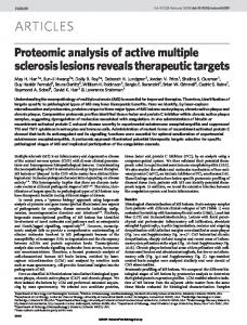
Introduction The problem of scheduling entails assigning an execution time (and sometimes a processor) to each of a set of actions with given durations, depending on a certain goal function (e.g. shortest schedule) and certain causal and resource constraints. The theory of scheduling has been investigated since the early 50s. The research so far can be divided into two categories: partitioning the set of all scheduling problems into (complexity) classes, and finding efficient algorithms for each class. Most of the problems being NP-complete, substantial effort has been spent on problem relaxations and heuristics to obtain algorithms that compute near-optimal schedules in polynomial time. But an axiomatization of the theory of scheduling still remains to be given. Here we outline such a calculus abstracting from both resource constraints and goal function and limiting the structure of the causal order. Our aim is to provide an axiom system that turns a process specification into a set of efficient (or semi-active) schedules [7]. These are the schedules that are potentially optimal for certain constraints and goal functions, provided the latter do not favor spending idle time. For simplicity, we consider only specifications in which no action has more than one immediate causal predecessor, i.e. the precedence graph has a multi-tree order. Viewed from a different angle, our approach can be described as applying concurrency theory to scheduling. A lot of algebras of concurrent processes have been given, e.g. ACP [3], CCS [11] or CSP [10]. Hence, one might ask why we develop a new calculus instead of using an existing one. The answer lies in the specific requirements of processes needed for scheduling: A scheduling calculus must include the notion of time, the concept of durational actions and the possibility to delay an action arbitrarily. Time has been incorporated into the calculi mentioned above (ACP [2], TCCS [12], TCSP [13]), but generally employing instantaneous actions. Durational actions are treated in [1, 9], for example, but these approaches do not allow actions to be delayed (or in the case of [9] only to wait for a synchronization partner). This means that in “a || b” actions a and b are always executed simultaneously whereas in scheduling they might as well be run sequentially in either order. In e.g. [4, 6], and in various references quoted in [6], semantics are given that allow for arbitrary delays, but they are not accompanied by an axiomatization. Moreover, nowhere in the process algebra literature a concept of efficiency is formalized resembling the one of [7]. Hence, a new algebra is necessary. We call it scheduling algebra and develop its theoretical framework in the following sections. An example process is given in fig. 1. Its algebraic term is: a; (b || c; d) || e.
Fig. 1. Example process
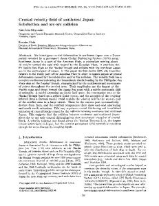
To visualize a schedule, the so-called GANTT chart [5] is used (see fig. 2). It depicts every action as a box labeled with its identifier. The length of the box indicates the duration of the action, and the placement of the box shows exactly when it takes place. In the scenario of fig. 2, actions a and d start simultaneously (on different processors), whereas c is executed immediately after a (and b after d). For the additional action e, the arrows indicate possible placements.
Fig. 2. GANTT diagram
Anchoring and efficiency A full-fledged scheduling problem consists of a specification, determining a set of valid schedules, some resource constraints, saying that certain actions cannot overlap in time, and a goal function, specifying how satisfactory certain schedules are. The objective is then to find an optimal schedule among the valid schedules that satisfy the resource constraints. Here we deal with scheduling problems in which the goal function and resource constraints are unspecified. We are interested in describing the valid schedules, and in finding, among the possibly infinite assortment of valid schedules, a finite subset, as small as possible, that for any choice of resource constraints and goal function contains an optimal schedule. In this quest, as is usual in scheduling theory, we limit attention to goal functions that do not favor spending idle time: a valid schedule, meeting the resource constraints, cannot improve by moving an action forwards in time. A schedule is called efficient (or semi-active) if it is valid and no actions can be moved backwards in time without violating validity or some hypothetical resource constraints. For the types of scheduling problems studied in this paper, as well as elsewhere in scheduling theory, every schedule can be “improved” to an efficient schedule by moving some of its actions backwards in time (cf. [7, theorem 2.1]). Depending on the goal function, this may not be a strict improvement, but it is never a regress. Thus the efficient schedules form the subclass of schedules sought above. However, in order to be of practical use, a more explicit characterization of the efficient schedules is needed. We call a schedule anchored if each action starts either at time 0 or at the termination time of some other process. Fig. 2 depicts an anchored schedule. If the execution times for the actions a to d is already given as indicated, an additional action e may start at time 0 if it does not use a resource required by either a or d. If e conflicts with a but not with d, it may begin execution upon termination of a (as drawn in fig. 2). So in total we have five possibilities for the starting time of e: 0 or the termination time of a, b, c or d. We call these points in time anchor points. It is easy to see that every anchored schedule s is efficient. If the resource constraints say that any two actions that do not overlap in s cannot overlap at all, it is impossible to preserve these resource constraints by moving actions backwards. Moreover, a goal function could be chosen that makes every schedule in which even one 2
action takes place later than in s less attractive than s itself, no matter what happens to the other actions. Conversely, for a special class of scheduling problems it is shown in [7] that all efficient schedules are anchored, i.e. that every valid schedule can be turned into a valid anchored one by moving actions backwards in time. Here we are interested in scheduling problems for which the same holds. For these the efficient schedules are exactly the anchored ones, and our efficiency operator can be implemented as an anchoring operator.
Syntax Let A be a set of atomic actions (external actions), and let T be the set of positive reals including zero. A pair (a, t) of A×T written as a(t) is called a time-stamped action or activity. It indicates that action a takes t units of time (the duration of a). The elements t of T also denote internal time actions which can be seen as silent steps (τ, t). Process terms can be constructed using the constants ε a(t)+ ∈ A×T
denoting the empty process, denoting the starting of action a with duration t,
the unary operators a(t)· t· ∆ [.]
Sequence, a(t)⋅ x meaning that x starts immediately after the execution of a, i.e. at time t, Time offset for t∈T; in t⋅ x the starting time of the actions in x is delayed by t time units and an anchor point at time t is added, Arbitrary delay operator, meaning that the prefixed process can be postponed indefinitely, Delay elimination, deleting every occurrence of the delay operator from the enclosed term by attaching the processes prefixed by ∆ to every possible anchor point,
and the binary operators ∪
∧,
Choice; x ∪ y denotes the execution of either x or y exclusively, forking of time (‘Hühnerfuß’ or ‘chicken claw’), an urgent parallel composition; x ∧, y means that the initial actions of both x and y start at the same time.
In addition, we use the following abbreviations: a(t);
||
(causal) precedence, a unary operator expressing linear order, so a(t); x says that x has to be executed some time (but not necessarily immediately) after completion of a. We have: a(t); x = a(t)⋅ ∆ x. concurrence, a binary operator expressing independence of processes. We have: x || y = ∆ x ∧, ∆ y.
The binding precedence of the binary operators (from loose to tight) is: ∪, || and ∧, . The unary operators bind tightest. Terms built from ε, a(t)+, a(t)⋅, t⋅, ∧, and [.] denote unique schedules. Choice between various schedules is introduced by the operators ∪ and ∆, and hence also by a(t); and ||. The delay elimination simply prunes some choices introduced by ∆. We take a, b to range over A×T∪A, t, u, v to range over T and x, y, z to range over all process expressions. For convenience, we sometimes abbreviate the expression a(t) by a. Moreover, we leave out trailing ε's in terms a(t)⋅ ε and t⋅ ε. Example: The expression a; b || c; d denotes two concurrent tasks, one executing first a and then b, and the other running c followed by d. Example schedules for the efficient process [a; b || c; d] are shown in fig. 3.
3
a⋅ c⋅ b⋅ d a⋅ b ∧, c⋅ d a⋅ ( c⋅ d ∧, b ) Fig. 3. Example schedules
As specification terms we consider processes P or [P] that contain no further occurrences of [.] and no direct occurrences of the sequencing operator a(t)⋅, although occurrences of a(t); are permitted. Let us call an occurrence of a(t)⋅ which can not be regarded as an occurrence of a(t); tight sequencing. Tight sequencing can be encoded with the delay elimination operator, namely a(t)⋅ b(t′) = [a(t)⋅ ∆b(t′)] = [a(t); b(t′)]. For these specification terms the argument of [7] showing that all efficient schedules are anchored applies, so that the delay elimination operator indeed describes efficiency. This need not be true for general processes. Consider for example the process ∆ a(1)⋅ b(1) || c(2). A valid schedule for this process specification is shown in fig. 4. This schedule is efficient because it is the shortest schedule for the given specification if we assume that b and c may not overlap due to a resource conflict. But at the same time it is not anchored because the starting time of action a does not coincide with the finishing time of any other action.
Fig. 4. An efficient schedule that is not anchored
Axiomatic System The axioms of scheduling algebra are listed below. Please note that “+” refers to the real number addition. Basic Axioms x ∪ (y ∪ z) = (x ∪ y) ∪ z
A1
x∪y = y∪x
A2
x∪x = x
A3
(x ∧, y) ∧, z = x ∧, (y ∧, z)
A4
x ∧, y = y ∧, x
A5
0⋅ x = x
Z1
x ∧, ε = x
Z2
t⋅ (x ∪ y) = t⋅ x ∪ t⋅ y
D1
∆ (x ∪ y) = ∆ x ∪ ∆ y
D2
x ∧, (y ∪ z) = x ∧, y ∪ x ∧, z
D3
Zero Axioms
Distributivity of choice
4
Normal Form Axioms
a(t)⋅ x = a(t)+ ∧, t⋅ x
N1
t⋅ x ∧, (t + u)⋅ y = t⋅ (x ∧, u⋅ y)
N2
∆ x ∧, ∆ y = ∆ (x ∧, ∆ y ∪ y ∧, ∆ x)
N3
Elimination of delay (anchor axioms) [x ∪ y] = [x] ∪ [y]
AA1
[a(t)+ ∧, x] = a(t)+ ∧, [x]
AA2
[t⋅ x] = t⋅ [x]
AA3
[∆ x] = [x]
AA4
[t⋅ x ∧, ∆ y] = [t⋅ x ∧, y] ∪ t⋅ [x ∧, ∆ y]
AA5
[ε] = ε
AA6
Proposition The following equation follows from applying N1, D1, D3 and N1 in the given order: a⋅ (x ∪ y) = a⋅ x ∪ a⋅ y
P1
The distributivity axioms and P1 indicate that we work in a linear-time setting. This is because we treat scheduling as a planning problem where all decisions (choices) are made prior to the execution of the process. Note that we do not have the axioms x ∪ ε = x and t⋅ u⋅ x = (t+u)⋅ x. They are not sound because the terms on the left side introduce an additional empty schedule and an anchor point at t, respectively. Example Applying the axioms, the definitions and P1 in a suitable order, we can compute the schedules for an example process specification. The penultimate equality shows the term in normal form (see below); the last equality gives the term in anchor form (explained later). Recall that we abbreviate a(t) by a, and that we leave out trailing ε’s. [ a(1); b(3) || c(2); d(1) ] = [ ∆( a(1)⋅ ∆b(3) ) ∧, ∆( c(2)⋅ ∆d(1) ) ] = a+ ∧, 1 ( b+ ∧, 3 ( c+ ∧, 2 ( d+ ∧, 1 ) ) ) a+ ∧, 1 ( c+ ∧, b+ ∧, 2⋅ 1 ( d+ ∧, 1 ) ) a+ ∧, 1 ( c+ ∧, 2 ( b+ ∧, ( d+ ∧, 1⋅ 2 ) ) ) c+ ∧, 2 ( a+ ∧, 1 ( b+ ∧, 3 ( d+ ∧, 1 ) ) ) c+ ∧, 2 ( a+ ∧, 1 ( d+ ∧, 1 ( b+ ∧, 3 ) ) ) c+ ∧, 2 ( d+ ∧, 1 ( a+ ∧, ( 1 ( b+ ∧, 3 ) ) ) ) c+ ∧, a+ ∧, 1 ( b+ ∧, 1 ( d+ ∧, 1⋅ 1 ) ) c+ ∧, a+ ∧, 1⋅ 1 ( d+ ∧, 1 ( b+ ∧, 3 ) )
∪ ∪ ∪ ∪ ∪ ∪ ∪ ∪
a+ ∧, 1 ( c+ ∧, b+ ∧, 2 ( d+ ∧, 1 ) ) a+ ∧, 1 ( c+ ∧, 2 ( b+ ∧, 3 ( d+ ∧, 1 ) ) ) a+ ∧, 1 ( c+ ∧, 2 ( d+ ∧, 1 ( b+ ∧, 3 ) ) ) c+ ∧, 2 ( a+ ∧, 1 ( d+ ∧, ( b+ ∧, 1⋅ 2 ) ) ) c+ ∧, 2 ( d+ ∧, a+ ∧, ( 1 ( b+ ∧, 3 ) ) ) c+ ∧, a+ ∧, 1 ( b+ ∧, 1⋅ 2 ( d+ ∧, 1 ) ) c+ ∧, a+ ∧, 1⋅ 1 ( b+ ∧, 3 ( d+ ∧, 1 ) ) c+ ∧, a+ ∧, 1⋅ 1 ( d+ ∧, ( b+ ∧, 1⋅ 2 ) )
∪ ∪ ∪ ∪ ∪ ∪ ∪ =
a⋅ b⋅ c⋅ d ∪ a⋅ c⋅ b⋅ d ∪ a⋅ c⋅ d⋅ b ∪ c⋅ a⋅ b⋅ d ∪ c⋅ a⋅ d⋅ b ∪ c⋅ d⋅ a⋅ b ∪ a⋅ ( c⋅ d ∧, b ) ∪ a⋅ ( b⋅ d ∧, c ) ∪ c⋅ ( a ∧, d⋅ b ) ∪ a⋅ c⋅ ( b ∧, d ) ∪ a⋅ b ∧, c⋅ d ∪ c⋅ a⋅ ( b ∧, d ) ∪ a ∧, c⋅ ( b ∧, d ) ∪ a ∧, c⋅ b⋅ d ∪ a ∧, c⋅ d⋅ b ∪ c ∧, a⋅ b⋅ d Normal form theorem
All terms can be written in the form ∪ N where 5
::= a(t)+ ∧, N | t⋅ N for t ≠ 0 | ∆N | for t ≠ 0 t⋅ N ∧, ∆ N | ε This normal form theorem is proved by structural induction on terms. We show for every operator that the composition of terms in normal form again yields a term that can be expressed in normal form. The choice operator distributes over every other operator (D1 - D3, P1, AA1) so that it can always be moved to the top level. This and associativity (A1) and commutativity (A2) allow us to denote every term as a union of choice-free subterms. Prefixing a normal term with ∆ or t⋅ (for t≠0) is by definition normal, as is ε. Z1 takes care of terms 0⋅ N. Using Z2, the constant a(t)+ can be written as the normal form a(t)+ ∧, ε. For a(t)⋅ N, axiom N1 leads to the normal form N
a(t)⋅ N = a(t)+ ∧, t⋅ N. Delay elimination is straightforward with AA1 - AA6. It remains to be shown that forking of normal terms can be normalized. Let K, L, M and N be normal terms. Then A4 IH → a(t)+ ∧, (M ∧, N) → a(t)+ ∧, N′, A5,Z2 ε ∧, N → N,
(a(t)+ ∧, M) ∧, N
where IH abbreviates induction hypothesis, and N′ denotes the normalization of M ∧, N. For the remaining 3 normal forms we have to prove normalization only for the upper triangle of the following matrix (due to commutativity of forking), in which t, u>0:
∧, t⋅ M
u⋅ K
∆K
u K ∧, ∆ L
N2 (t ≤ u), IH
√
A4, N2 (t ≤ u), IH
N3, IH, IH
A5, A4, N3, IH, IH
∆M t M ∧, ∆ N
A4, A4, A5, A4, A4, N2 (t ≤ u), N3, IH, IH, IH
Table 1. Normal form proofs
The proof proceeds applying the laws stated modulo commutativity (√ means that the term is already in normal form).
Semantics As a semantic model, we define schedules similar to the real-time execution sequences in [13]. Each expression maps to a set of possible schedules: A×T×T × 2T × 2T−{0} [[.]]: Expr → 2IN
A schedule is a triple σ = 〈σ0; σ1; σ2〉 where σ0 is a multi-set over triples (action, duration, starting time), σ1 is a set of starting and finishing times and σ2 a set of anchor points (or finishing times), excluding 0. Because 0 is always an anchor point, there is no need to record it explicitly; suppressing it turns out to have technical advantages. Typically, we leave out the brackets delimiting σ0, σ1 and σ2, i.e. [[ a(1)⋅ b(2) ∧, a(1) ]] = { 〈 (a, 1, 0), (a, 1, 0), (b, 2, 1) ; 0, 1, 3 ; 1, 3 〉 }. This schedule is interpreted as follows: • • • •
a(1) is started twice at time 0, b(2) at time 1 (immediately after a), the starting times are 0 and 1 (for a and b respectively) and the anchor points are 1 and 3 (the finishing times of a and b respectively).
6
Because Z1 yields a(1)⋅ b(2) = a(1)⋅ b(2)⋅ 0 and the latter term has a starting time 3 (for the internal action of duration 0), 3 can be regarded as a potential starting time of the process a(1)⋅ b(2) as well. For this reason we include in σ1 not only the starting times, but also the finishing times of actions. For two schedules σ and ρ, we write σ∪ρ for 〈 σ0∪ρ0 ; σ1∪ρ1 ; σ2∪ρ2 〉. The offset of a schedule by a fixed amount of time is defined by: σ + u = 〈 {| (a, t, p + u) (a, t, p) ∈ σ0 |} ; { p + u p∈ σ1 } ; { p + u p∈ σ2 } 〉. The general definition of the semantics is as follows: [[ ε ]] = { 〈 ∅ ; 0 ; ∅ 〉 }
(1)
[[ a(t)+ ]] = { 〈 (a, t, 0) ; 0 ; ∅ 〉 }
(2)
[[ a(t)⋅ P ]] = { 〈 (a, t, 0) ; 0 ; {t}−{0} 〉 ∪ (σ + t) σ ∈ [[P]] }
(3)
[[ t⋅ P ]] = { 〈 ∅ ; 0 ; {t}−{0} 〉 ∪ (σ + t) σ ∈ [[P]] }
(4)
[[ ∆P ]] = { 〈 ∅ ; 0 ; ∅ 〉 ∪ (σ + u) σ ∈ [[P]], u ∈ T }
(5)
[[ [P] ]] = { σ ∈ [[P]] σ1 ⊂ σ2∪{0} }
(6)
[[ P ∪ Q ]] = [[P]] ∪ [[Q]]
(7)
[[ P ∧, Q ]] = { σ ∪ ρ σ ∈ [[P]], ρ ∈ [[Q]] }
(8)
Note that this definition ensures that 0 ∈ σ1, 0 ∉ σ2 and σ2 ⊂ σ1, for all schedules σ. The role of the elimination operator [.] A term not containing [.] represents a set of schedules, both efficient and inefficient ones. Delay elimination restricts attention to the efficient schedules, thereby eliminating all schedules known not to be optimal under any goal function or constraints. On the syntactical level, this corresponds to the elimination of ∆’s, which is achieved by the operator [.]. One might ask why this is not done implicitly, i.e. by giving every term p the semantics of [p]. The answer is that the following implication does not hold: [[ [x] ]] = [[ [y] ]] ⇒ [[ [x || z] ]] = [[ [y || z] ]]. A counterexample to the implication can be constructed easily by setting: x = a(1)⋅ b(1), y = a(1)⋅ ∆ b(1), z = c(1). We then get: [[ [a(1)⋅ b(1)] ]] = { 〈 (a, 1, 0), (b, 1, 1) ; 0, 1, 2 ; 1, 2 〉 } = [[ [a(1)⋅ ∆ b(1)] ]], but: 〈 (a, 1, 0), (b, 1, 2), (c, 1, 1) ; 0, 1, 2, 3 ; 1, 2, 3 〉 ∈ [[ [a(1)⋅ ∆ b(1) || c(1)] ]], 〈 (a, 1, 0), (b, 1, 2), (c, 1, 1) ; 0, 1, 2, 3 ; 1, 2, 3 〉 ∉ [[ [a(1)⋅ b(1) || c(1)] ]].
Correctness Axioms A1 to A3 are correct w.r.t. our schedule semantics because set union is associative, commutative and idempotent. Associativity and commutativity of multi-set union yield A4 and A5. Z1 and Z2 are explained by 0 and the empty set being the neutral elements of addition and (multi-)set union respectively, taking into account that 0 is already in σ1 for every schedule σ. Correctness of D1 can be derived as follows: [[ t⋅ (x ∪ y) ]] = { 〈 ∅ ; 0 ; {t}−{0} 〉 ∪ (σ + t) σ ∈ [[x ∪ y]] } = { 〈 ∅ ; 0 ; {t}−{0} 〉 ∪ (σ + t) σ ∈ [[x]] ∪ [[y]] } 7
= { 〈 ∅ ; 0 ; {t}−{0} 〉 ∪ (σ + t) σ ∈ [[x]] } ∪ { 〈 ∅ ; 0 ; {t}−{0} 〉 ∪ (σ + t) σ ∈ [[y]] } = [[ t⋅ x ]] ∪ [[ t⋅ y ]] = [[ t⋅ x ∪ t⋅ y ]] The proofs of D2 and D3 proceed analogously. For N1 - N3 and AA1 - AA6, we have: [[ a(t)⋅ x ]]
= = = =
{ 〈 (a, t, 0) ; 0 ; {t} − {0} 〉 ∪ (σ + t) σ ∈ [[ x ]] } { 〈 (a, t, 0) ; 0 ; ∅ 〉 ∪ ( 〈 ∅ ; 0 ; {t} − {0} 〉 ∪ (σ + t) ) σ ∈ [[ x ]] } { 〈 (a, t, 0) ; 0 ; ∅ 〉 ∪ ρ ρ ∈ [[ t⋅ x ]] } [[ a(t)+ ∧, t⋅ x ]]
[[ t⋅ x ∧, (t + u)⋅ y ]] = { σ ∪ ρ σ ∈ [[ t⋅ x ]], ρ ∈ [[ (t + u)⋅ y ]] } = { 〈 ∅ ; 0 ; {t} − {0} 〉 ∪ (π + t) ∪ 〈 ∅ ; 0 ; {t + u} − {0} 〉 ∪ (ω + t + u) π ∈ [[ x ]], ω ∈ [[ y ]] } =1 { 〈 ∅ ; 0 ; {t} − {0} 〉 ∪ (π + t) ∪ 〈 ∅ ; t ; {t + u} − {0} 〉 ∪ (ω + t + u) π ∈ [[ x ]], ω ∈ [[ y ]] } =2 { 〈 ∅ ; 0 ; {t} − {0} 〉 ∪ (π + t) ∪ 〈 ∅ ; t ; {t + u} − {t} 〉 ∪ (ω + t + u) π ∈ [[ x ]], ω ∈ [[ y ]] } = { 〈 ∅ ; 0 ; {t} − {0} 〉 ∪ (π + t) ∪ ( 〈 ∅ ; 0 ; {u} − {0} 〉 + t ) ∪ (ω + t + u) π ∈ [[ x ]], ω ∈ [[ y ]] } = { 〈 ∅ ; 0 ; {t} − {0} 〉 ∪ ( π ∪ 〈 ∅ ; 0 ; {u} − {0} 〉 ∪ (ω + u) ) + t π ∈ [[ x ]], ω ∈ [[ y ]] } = { 〈 ∅ ; 0 ; {t} − {0} 〉 ∪ ( ( π ∪ ρ ) + t ) π ∈ [[ x ]], ρ ∈ [[ u⋅ y ]] }
(
)
{ 〈 ∅ ; 0 ; {t} − {0} 〉 ∪ (σ + t) σ ∈ [[ x ∧, u⋅ y ]] } [[ t⋅ (x ∧, u⋅ y) ]] [[ ∆ x ∧, ∆ y ]] = { σ ∪ ρ σ ∈ [[ ∆ x ]], ρ ∈ [[ ∆ y ]] } = { 〈 ∅ ; 0 ; ∅ 〉 ∪ (π + t) ∪ (ω + u) π ∈ [[ x ]], ω ∈ [[ y ]], t, u ∈ T } =1 { 〈 ∅ ; 0, t ; ∅ 〉 ∪ (π + t) ∪ (ω + u) π ∈ [[ x ]], ω ∈ [[ y ]], t ≤ u } ∪ { 〈 ∅ ; 0, u ; ∅ 〉 ∪ (π + t) ∪ (ω + u) π ∈ [[ x ]], ω ∈ [[ y ]], t ≥ u } =3 { 〈 ∅ ; 0 ; ∅ 〉 ∪ ( π ∪ 〈 ∅ ; 0 ; ∅ 〉 ∪ (ω + v) ) + t π ∈ [[ x ]], ω ∈ [[ y ]], t, v ∈ T } ∪ = =
( ) { 〈 ∅ ; 0 ; ∅ 〉 ∪ ( ( ω ∪ 〈 ∅ ; 0 ; ∅ 〉 ∪ (π + w) ) + u ) π ∈ [[ x ]], ω ∈ [[ y ]], u, w ∈ T }
=
{ 〈 ∅ ; 0 ; ∅ 〉 ∪ ( ( π ∪ ρ ) + t ) π ∈ [[ x ]], ρ ∈ [[ ∆ y ]], t ∈ T } ∪
{ 〈 ∅ ; 0 ; ∅ 〉 ∪ ( ( ω ∪ σ ) + u ) σ ∈ [[ ∆ x ]], ω ∈ [[ y ]], u ∈ T } = { 〈 ∅ ; 0 ; ∅ 〉 ∪ (ψ + t) ψ ∈ [[ x ∧, ∆ y ]], t ∈ T } ∪ { 〈 ∅ ; 0 ; ∅ 〉 ∪ (ζ + u) ζ ∈ [[ ∆ x ∧, y ]], u ∈ T } = [[ ∆ (x ∧, ∆ y) ]] ∪ [[ ∆ (y ∧, ∆ x) ]] = [[ ∆ (x ∧, ∆ y ∪ y ∧, ∆ x) ]] = [[ [x ∪ y] ]] { σ ∈ [[ x ∪ y ]] σ1 ⊂ σ2 ∪ {0} } = { σ ∈ [[ x ]] ∪ [[ y ]] σ1 ⊂ σ2 ∪ {0} } = { σ ∈ [[ x ]] σ1 ⊂ σ2 ∪ {0} } ∪ { σ ∈ [[ y ]] σ1 ⊂ σ2 ∪ {0} } = [[ [x] ]] ∪ [[ [y] ]] = [[ [x] ∪ [y] ]] + , [[ [a(t) ∧ x] ]] = { σ ∈ [[ a(t)+ ∧, x ]] σ1 ⊂ σ2 ∪ {0} } = { 〈 (a, t, 0) ; 0 ; ∅ 〉 ∪ ρ ρ ∈ [[ x ]], ρ1 ∪ {0} ⊂ ρ2 ∪ ∅ ∪ {0} } = { 〈 (a, t, 0) ; 0 ; ∅ 〉 ∪ ρ ρ ∈ [[ x ]], ρ1 ⊂ ρ2 ∪ {0} } = { 〈 (a, t, 0) ; 0 ; ∅ 〉 ∪ σ σ ∈ [[ [x] ]] } = [[ a(t)+ ∧, [x] ]] = [[ [t⋅ x] ]] { σ ∈ [[ t⋅ x ]] σ1 ⊂ σ2 ∪ {0} } = { 〈 ∅ ; 0 ; {t} − {0} 〉 ∪ (ρ + t) ρ ∈ [[ x ]], (ρ1 + t) ∪ {0} ⊂ (ρ2 + t) ∪ {t, 0} } = { 〈 ∅ ; 0 ; {t} − {0} 〉 ∪ (ρ + t) ρ ∈ [[ x ]], ρ1 ⊂ ρ2 ∪ {0} } = { 〈 ∅ ; 0 ; {t} − {0} 〉 ∪ (ρ + t) ρ ∈ [[ [x] ]] } = [[ t⋅ [x] ]] = [[ [∆ x] ]] { σ ∈ [[ ∆ x ]] σ1 ⊂ σ2 ∪ {0} } 1 2 3
We always have that 0∈π1, hence t∈π1+t. We leave it to the reader to check ({t} − {0}) ∪ ({t + u} − {0}) = ({t} − {0}) ∪ ({t + u} − {t}). In the first line we write t + v for u. In the second we replace t by u + w.
8
= =4 =5 =
{ 〈 ∅ ; 0 ; ∅ 〉 ∪ (ρ + u) ρ ∈ [[ x ]], u ∈ T, (ρ1 + u) ∪ {0} ⊂ (ρ2 + u) ∪ {0} } { 〈 ∅ ; 0 ; ∅ 〉 ∪ ρ ρ ∈ [[ x ]], ρ1 ⊂ ρ2 ∪ {0} } { ρ ρ ∈ [[ x ]], ρ1 ⊂ ρ2 ∪ {0} } [[ [x] ]]
[[ [t⋅ x ∧, ∆ y] ]] = { σ ∈ [[ t⋅ x ∧, ∆ y ]] σ1 ⊂ σ2 ∪ {0} } = { ρ ∪ ω ρ ∈ [[ t⋅ x ]], ω ∈ [[ ∆ y ]], ρ1 ∪ ω1 ⊂ ρ2 ∪ ω2 ∪ {0} } = { 〈 ∅ ; 0 ; {t} − {0} 〉 ∪ (ψ + t) ∪ (π + u) ψ ∈ [[ x ]], π ∈ [[ y ]], u ∈ T, (ψ1 + t) ∪ (π1 + u) ∪ {0} ⊂ (ψ2 + t) ∪ (π2 + u) ∪ {t, 0} } = { 〈 ∅ ; 0 ; {t} − {0} 〉 ∪ (ψ + t) ∪ (π + u) ψ ∈ [[ x ]], π ∈ [[ y ]], (ψ1 + t) ∪ (π1 + u) ⊂ (ψ2 + t) ∪ (π2 + u) ∪ {t, 0}, u < t } ∪ { 〈 ∅ ; 0 ; {t} − {0} 〉 ∪ (ψ + t) ∪ (π + u) ψ ∈ [[ x ]], π ∈ [[ y ]], (ψ1 + t) ∪ (π1 + u) ⊂ (ψ2 + t) ∪ (π2 + u) ∪ {t, 0}, u ≥ t } =6 { 〈 ∅ ; 0 ; {t} − {0} 〉 ∪ (ψ + t) ∪ π ψ ∈ [[ x ]], π ∈ [[ y ]], (ψ1 + t) ∪ π1 ⊂ (ψ2 + t) ∪ π2 ∪ {t, 0} } ∪ { 〈 ∅ ; 0 ; {t} − {0} 〉 ∪ (ψ+ t) ∪ (π + t + v) ψ ∈ [[ x ]], π ∈ [[ y ]], (ψ1 + t) ∪ (π1 + t + v) ⊂ (ψ2 + t) ∪ (π2 + t + v) ∪ {t, 0}, v ∈ T } = { ω ∪ π ω ∈ [[ t⋅ x ]], π ∈ [[ y ]], ω1 ∪ π1 ⊂ ω2 ∪ π2 ∪ {0} } ∪ { 〈 ∅ ; 0 ; {t} − {0} 〉 ∪ ( ψ ∪ (π + v) ) + t ψ ∈ [[ x ]], π ∈ [[ y ]], ( ψ1 ∪ (π1 + v) ) + t ⊂ ( ψ2 ∪ (π2 + v) ∪ {0} ) + t ∪ {0}, v ∈ T } = { σ σ ∈ [[ t⋅ x ∧, y ]], σ1 ⊂ σ2 ∪ {0} } ∪ { 〈 ∅ ; 0 ; {t} − {0} 〉 ∪ ( ( ψ ∪ ρ ) + t ) ψ ∈ [[ x ]], ρ ∈ [[ ∆ y ]], (ψ ∪ ρ ) + t ⊂ ( ψ ∪ ρ ∪ {0} ) + t }
(
= ∪
(
)
)
1
[[ [t⋅ x ∧, y] ]]
1
2
2
{ 〈 ∅ ; 0 ; {t} − {0} 〉 ∪ ( ( ψ ∪ ρ ) + t ) ψ ∈ [[ x ]], ρ ∈ [[ ∆ y ]], ψ1 ∪ ρ1 ⊂ (ψ2 ∪ ρ2) ∪ {0} } = [[ [t⋅ x ∧, y] ]] ∪ { 〈 ∅ ; 0; {t} − {0} 〉 ∪ (σ + t) σ ∈ [[ x ∧, ∆ y ]], σ1 ⊂ σ2 ∪ {0} } = [[ [t⋅ x ∧, y] ]] ∪ { 〈 ∅ ; 0; {t} − {0} 〉 ∪ (σ + t) σ ∈ [[ [x ∧, ∆ y] ]] } = [[ [t⋅ x ∧, y] ]] ∪ [[ t⋅ [x ∧, ∆ y] ]] = [[ [t⋅ x ∧, y] ∪ t⋅ [x ∧, ∆ y] ]] [[ [ε] ]] = { 〈 ∅ ; 0 ; ∅ 〉 {0} ⊂ ∅ ∪ {0} } = [[ ε ]]
Completeness w.r.t. ∆-free terms In this section, we will prove completeness of the axiomatic system for ∆-free terms. The normal form theorem allows restriction to ∆-free normal forms, which, for example, arise from normalizing arbitrary terms of the form [P]. Each choice-free subterm of such a term corresponds uniquely to a set of only one schedule. Lemma 1. Let N be a term of the form N ::= a(t)+ ∧, N | t⋅ N | ε, where t ≠ 0. Then | [[ N ]] | = 1. Proof by structural induction: | [[ ε ]] | = | { 〈 ∅ ; 0 ; ∅ 〉 } | = 1. [[ t⋅ N ]] = { 〈 ∅ ; 0 ; {t}−{0} 〉 ∪ (σ + t) σ ∈ [[N]] }. So if | [[ N ]] | = 1, then | [[ t⋅ N ]] | = 1. The case a(t)+ ∧, N proceeds likewise.
4 5 6
Since 0∈ρ1 and 0∉ρ2, we have u ∈ (ρ1+u) ⊂ (ρ2 + u) ∪ {0} but u ∉ ρ2 + u, hence u ∈ {0}. Because always 0∈ρ1. Since 0∈π1 and 0∉π2, we have u ∈ (π1+u) ⊂ (ψ2 + t) ∪ (π2 + u) ∪ {t, 0} but u ∉ (ψ2 + t) ∪ (π2 + u) ∪ {t} provided u0, and M = b1(u1)+ ∧, b2(u2)+ ∧, … ∧, bm(um)+ ∧, M′ with M′ = ε or M′ = u⋅ M′′ with u>0. Let σ be the unique schedule in [[N]] = [[M]]. We have N′ = ε ⇔ σ2 = ∅ ⇔ M′ = ε. In case N′ = M′ = ε we have σ0 = {| (a1, t1, 0), (a2, t2, 0), …, (an, tn, 0) |} = {| (b1, u1, 0), (b2, u2, 0), …, (bm, um, 0) |}. Hence {| a1(t1)+, a2(t2)+, …, an(tn)+ |} = {| b1(u1)+, b2(u2)+, …, bm(um)+ |}, so in particular n = m. It follows that A4, A5 N = M. In case N′ = t⋅ N′′ and M′ = u⋅ M′′ we have [[ N ]] = { 〈 (a1, t1, 0), (a2, t2, 0), …, (an, tn, 0) ; 0 ; t 〉 ∪ (σ + t) σ ∈ [[N′′]] } and [[ M ]] = { 〈 (b1, u1, 0), (b2, u2, 0), …, (bm, um, 0) ; 0 ; u 〉 ∪ (ρ + u) ρ ∈ [[M′′]] }. Again it follows that {| a1(t1)+, a2(t2)+, …, an(tn)+ |} = {| b1(u1)+, b2(u2)+, …, bm(um)+ |}, so in particular n = m. Furthermore, we have u = t because t is the least anchor point in the unique schedule of [[N]], and so is u for [[M]]. Finally, [[N′′]] = [[M′′]], and therefore by induction A4, A5 N′′ = M′′. Hence A4, A5 N = M. Theorem. Let K, L be ∆-free normal forms with [[K]] = [[L]] then A1, …, A5 K = L. Proof: Using A1, A2, A3, it suffices to show that for every choice-free subterm N of K there is a choice-free subterm M of L such that A4, A5 N = M (and vice versa). By lemma 1, [[N]] = {σ}, so σ ∈ [[K]] = [[L]]. Again by lemma 1, there is a choice-free subterm M of L such that [[M]] = {σ} = [[N]]. Now, by lemma 2, A4, A5 N = M.
Anchor Form For every t-free term [P] we can eliminate [.] without introducing time offsets. P is t-free ⇒ ∃Q: Q = [P] where Q contains neither [.] nor t⋅ We call this the anchor form of a term because all schedules are given by just anchoring actions to the endpoints of others. The GANTT chart can be drawn easily from this form. Using a straightforward structural induction, one can establish that for every schedule σ of a t-free term we have ∀t∈σ2: ∃(a, u, v)∈σ0: t = u + v with u > 0.
(*)
Furthermore, employing N2, Z2 and again N2, we obtain t⋅ (u⋅ x ∧, v⋅ y) = t⋅ ε ∧, (t+u)⋅ x ∧, (t+v)⋅ y. Every term [P] can be written in a ∆-free normal form, which, using structural induction, Z1 and the law above, can be converted to a sum of terms of the form u1⋅ a1(t1)+ ∧, u2⋅ a2(t2)+ ∧, … ∧, uk⋅ ak(tk)+ ∧, uk+1⋅ ε ∧, uk+2⋅ ε ∧, … ∧, un⋅ ε. Assuming P is t-free, (*) implies that for every ui > 0 there exists a j ∈ {1, … k} such that ui = uj + tj and tj > 0. We will remove step by step the time offsets ui⋅ in the term above, starting with the largest, until only time offsets 0⋅ remain. The intermediate terms encountered during this process will always remain in the form u1⋅ a1(t1)+ ∧, u2⋅ a2(t2)+ ∧, … ∧, uk⋅ ak(tk)+ ∧, uk+1⋅ Nk+1 ∧, uk+2⋅ Nk+2 ∧, … ∧, un⋅ Nn
(**)
where for every ui > 0 there exists a j ∈ {1, … k} such that ui = uj + tj, tj > 0 and the Ni contain neither time offsets nor occurrences of [.] or ∆. 10
Let v > 0 be the maximum of { u1, u2, … un }, and let j ∈ {1, … k} be such that v = uj + tj and tj > 0. Using A4-5, we write all subterms ui⋅ ai(ti) and ui⋅ Ni with ui = v as well as uj⋅ aj(tj) at the right of the formula, thus obtaining an expression of the form u′1⋅ a′1(t′1)+ ∧, u′2⋅ a′2(t′2)+ ∧, … ∧, u′l⋅ a′l(t′l)+ ∧, u′l+1⋅ N′l+1 ∧, u′l+2⋅ N′l+2 ∧, … ∧, u′m⋅ N′m ∧, K with K = uj⋅ aj(tj)+ ∧, v⋅ M1 ∧, v⋅ M2 ∧, … ∧, v⋅ Mh. Using axioms N2 and Z1, K can be rewritten as uj⋅ aj(tj)+ ∧, v⋅ (M1 ∧, M2 ∧, … ∧, Mh) and, with N1, as uj⋅ aj(tj)⋅ (M1 ∧, M2 ∧, … ∧, Mh). This brings the term again in the form (**) and we can continue with the next-largest member of { u1, u2, … un }. In the end, all remaining ui's will be 0 and Z1 turns the term into the required form. Example Consider the term [ a; (b || c) || d ] where all actions consume one unit of time. Transformation of this term into its anchor form yields 19 possible schedules. They are shown in fig. 5 grouped into the three basic orders “a; (b || c)”, “a; b; c” and “a; c; b” with the independent action d attached to an anchor point or inserted in front of or in between the other actions. This example might suggest that it is possible to convert a t-free term [P] into its anchor form without considering the duration of its actions. However, this is not possible in general: the anchor form of the term [ a(1); b(3) || c(2); d(1) ] that has been calculated in a previous example contains the schedule a(1) ∧, c(2)⋅ ( b(3) ∧, d(1) ), but not a(1)⋅ ( b(3) ∧, d(1) ) ∧, c(2).
Fig. 5. All schedules
Term Rewriting We show that modulo associativity and commutativity of choice and Hühnerfuß our axioms, when read from left to right, form a confluent and (strongly) normalizing rewrite system, provided that we add the rewrite rule [a(t)+] → a(t)+ (which is derivable from the axiom system). If we drop the rewrite rule A3 (the idempotence of choice), the normal forms are exactly the normal forms in the sense of our normal form theorem, except that all subterms a(t)+ ∧, ε are replaced by a(t)+ (so a(t)+ is a normal form for the rewrite system). In the presence of A3 the same normal forms apply, but without pairs of summands that are equal modulo A4 and A5. It is easy to check that such normal forms allow no further rewriting; the proof of the normal form theorem (but omitting the reverse application of Z2) shows essentially that all other terms can be rewritten into a normal form. Thus the rewrite system is normalizing. Here we omit the proof that it is even strongly normalizing; however, it involves only standard term rewriting techniques. Confluence for terms of the form [P] follows immediately from the proof of our completeness theorem for such terms (because only the axioms A1-5 are involved in the completeness proof for ∆-free normal forms). Confluence for the entire rewrite system can be established by the Knuth-Bendix method, skipping pairs of 11
overlapping redexes that lay within a term of the form [P]. In the table 2, we review the relevant pairs of overlapping redexes. A3 with D1, D2 and D3
trivial
Z1 with D1 and N2 (in two ways)
trivial
Z2 with D3 and Z2
trivial
D1 with N2 (in two ways)
trivial with D3
D2 with N3 (in two ways)
trivial with D3
D3 with D3
trivial
N2 with itself
OK
N3 with itself
OK
Table 2. Overlapping redexes
An implementation of the system without A3 can be found at the URL
http://www.uni-koblenz.de/~rittgen/SA.html. This applet generates the normal form for the axiom system given any term of your chosing.
Conclusion In this paper, we have proposed a calculus for durational actions, namely scheduling algebra. The constants and operators of this algebra allow to specify process terms as a multi-tree order over actions with a certain duration. A normal form exists for each term which for ∆-free terms is unique modulo A1-5. Using the axioms of this calculus, the set of all efficient schedules [P] can be “computed” for any process P without tight sequencing. The operator [.] does so by generating a subterm (schedule) for any possible attachment of actions to anchor points, thus eliminating all time delays ∆. We established soundness of the axiomatic system w.r.t. a schedule semantics and showed that the algebra is complete for ∆-free terms (sets of schedules), such as arise from terms of the form [P]. Currently, our calculus is designed for multi-tree precedence. To extend it to arbitrary orders (with more than one predecessor to an action), synchronization must be present in the algebra (as follows from the existence of partial orders which are not “series-parallel” [8]). This is left for future research.
References 1. Aceto, L.; Murphy, D.: Timing and Causality in Process Algebra, Acta Informatica 33, 1996, pp. 317-350 2. Baeten, J.C.M.; Bergstra, J.A.: Real Time Process Algebra, Formal Aspects of Computing 3(2), 1991, pp. 142-188 3. Bergstra, J.A.; Klop, J.W.: Process Algebra for Synchronous Communication, Information and Control 60, 1984, pp. 109-137 4. Chen, X.J.; Corradini, F.; Gorrieri, R.: A Study on the Specification and Verification of Performance Properties, Proceedings of AMAST ’96, Lecture Notes in Computer Science 1101, Springer, Berlin, 1996, pp. 306-320 5. Clark, W.: The Gantt Chart: A Working Tool of Management, Pitman, London, 1935 6. Corradini, F.: On Performance Congruences for Process Algebras, Information and Computation 145(2), 1998, pp. 191230 7. French, S.: Sequencing and Scheduling: An Introduction to the Mathematics of the Job-Shop, Ellis Horwood, Chichester, 1982 8. Gischer, J.L.: The Equational Theory of Pomsets, Theoretical Computer Science 61, 1988, pp. 199-224 9. Gorrieri, R.; Roccetti, M.; Stancampiano, E.: A Theory of Processes with Durational Actions, Theoretical Computer Science 140(1), 1995, pp. 73-94 10. Hoare, C.A.R.: Communicating Sequential Processes, Prentice Hall, Englewood Cliffs, 1985 11. Milner, R.: A Calculus of Communicating Systems, Lecture Notes in Computer Science 92, Springer, Berlin, 1980 12. Moller, F.; Tofts, C.: A Temporal Calculus of Communicating Systems, in: Baeten, J.C.M.; Klop, J.W.: Proceedings of CONCUR '90, Lecture Notes in Computer Science 458, Springer, Berlin, 1990, pp. 401-415 13. Reed, G.M.; Roscoe, A.W.: A Timed Model for Communicating Sequential Processes, Theoretical Computer Science 58, 1988, pp. 249-261
12