Computer vision is a compilation of inference problems: given an image or a set ...... work is given by the generalized gradient vector flow of Xu and Prince [211].
Combinatorial Solutions for Shape Optimization in Computer Vision
Dissertation zur Erlangung des Doktorgrades (Dr. rer. nat.) der Mathematisch-Naturwissenschaftlichen Fakult¨at der Rheinischen Friedrich-Wilhelms-Universit¨at Bonn
vorgelegt von Thomas Schoenemann aus M¨ unster Bonn, im Dezember 2008
Angefertigt mit Genehmigung der Mathematisch-Naturwissenschaftlichen Fakult¨at der Rheinischen Friedrich-Wilhelms-Universit¨at Bonn.
1. Referent: Prof. Dr. Daniel Cremers 2. Referent: Prof. Hiroshi Ishikawa, Ph.D. Tag der Promotion: 27. April 2009. Diese Dissertation ist auf dem Hochschulserver der ULB Bonn unter http://hss.ulb.uni-bonn.de/diss_online elektronisch publiziert. Erscheinungsjahr: 2009.
Foreword Like all Ph.D. students, I submit this thesis with the aim to obtain a Ph.D. Yet, I have also come to value such theses as a useful means to get to know a new scientific field. After all I once got into this field by reading the Ph.D. thesis of my present supervisor, and this has greatly helped me to find the topic I want to be working on. For this reason I have tried to keep this thesis understandable to students in computer science, so that I could have understood it when I finished my studies. I probably only partially succeeded in that - the foremost aim is still to present the contributions I made in the last three years. To further help students about to finish their studies, I want to address a topic I found absent in all theses so far: Should I write a Ph.D. thesis? In my view you are definitely qualified if you provide the following three prerequisites: (1) good or excellent grades during your studies, preferably without having worked to exhaustion, (2) the desire never to stop learning and (3) the desire to contribute, even if you have doubts you are capable to. Once you started, do not expect to contribute much during the first year. In my experience it takes about a year until you see some loose ends. That is, you no longer just see unsolved problems, you start to realize that some of them can be solved – or at least improved. I hope this thesis convinces you that in computer vision many improvements are possible. In any case I hope this thesis finds a broad audience. For readers who want to deepen their knowledge I have compiled a list of books I consider good starting points. For combinatorial optimization I recommend [45], more advanced readers may also consider [137]. And for continuous optimization I recommend [21]. Books on computer vision include [194] and [107].
3
Acknowledgments Although I am the sole author of this thesis, naturally many people have contributed to make it possible, and they should be acknowledged here. My foremost credit goes to my supervisor, Prof. Dr. Daniel Cremers. I would like to thank him for making me think about energy minimization, teaching me how to write things down, supporting me during all this time and never losing faith in me and my ideas. Many thanks also to Prof. Hiroshi Ishikawa, Ph.D., for agreeing to review my thesis and publishing all the results I have built on in this thesis. I would also like to thank Prof. Dr.-Ing. Hermann Ney who supervised my diploma thesis. Although I did not have contact with him since I left his group, many of the ideas in this work arose from what I have learned from him. Someone I have not yet had the chance to work with is Prof. Dr. Fredrik Kahl. I hope this will change in the future. Many thanks also to my closest co-workers Prof. Dr. Simon Masnou, Frank R. Schmidt and Dr. Thomas Pock. The many discussions with them have much helped to improve the respective projects and also my understanding of the underlying theories. I would also like to thank Dr. Thomas Brox - although we have never published together, I have learned a lot from him. Furthermore I am indebted to Dr. Bastian Goldl¨ ucke, Dr. Thomas Pock, Frank R. Schmidt and Frank Steinbr¨ ucker who have proof-read an early version of this thesis and provided many valuable comments. Many thanks also to my family and friends for supporting me in my private life during the last three years. Especially I would like to thank my mother for proof-reading the final manuscript. My final acknowledgment goes to all the people worldwide who are willing to share their work with the world without asking for payment. In particular this includes all open source programmers and the authors of Wikipedia. Their invaluable work provides an important basis for research and has greatly helped to produce this thesis.
4
Notational Conventions Throughout this thesis vectors variables appear in bold face, i.e. I write x ∈ R2 , but x ∈ R. The same rule applies to vector-valued functions, i.e. g : R → R2 but g : R300 → R. The transpose of a vector v is denoted v⊤ . Unless otherwise stated the expression |v| will denote the L2 -norm (or Euclidean norm) of the finite-dimensional vector v. For infinitedimensional vectors (curves) this Euclidean norm is denoted as kCk to distinguish it from the one-dimensional measure |C| of a set C ⊆ R2 . The vector inequality v ≥ w expresses that vi ≥ wi for all i. The set R+ denotes the set of real numbers greater than 0, the set R+ 0 the set of real numbers greater than or equal to 0. Similarly, the set N denotes the set of integer numbers greater than or equal to 0 and N+ all integer numbers greater than 0. I intensively use the Kronecker symbol (for k, l ∈ N) δ(k, l) =
(
1 0
if k = l . else
An important notion for this thesis is the image gradient. For a signal I : R2 → gradient ∇I(x) at the place x = (x y)⊤ ∈ R2 is defined as the vector
∇I(x) =
∂I ∂x ∂I ∂y
=
I(x+ǫ,y)−I(x,y) ǫ ǫ→0 I(x,y+ǫ)−I(x,y) lim ǫ ǫ→0
lim
R, the
.
The reader is furthermore assumed familiar with basic knowledge in complexity analysis, in particular the O-notation to analyze the worst-case run-time of an algorithm. For an introduction see [187]. Lastly I assume some basic knowledge about graphs and about convex functions. In particular it will be of importance that convex functions can be optimized globally, e.g. via gradient descent.
5
Abstract This thesis aims at solving so-called shape optimization problems, i.e. problems where the shape of some real-world entity is sought, by applying combinatorial algorithms. I present several advances in this field, all of them based on energy minimization. The addressed problems will become more intricate in the course of the thesis, starting from problems that are solved globally, then turning to problems where so far no global solutions are known. The first two chapters treat segmentation problems where the considered grouping criterion is directly derived from the image data. That is, the respective data terms do not involve any parameters to estimate. These problems will be solved globally. The first of these chapters treats the problem of unsupervised image segmentation where apart from the image there is no other user input. Here I will focus on a contour-based method and show how to integrate curvature regularity into a ratio-based optimization framework. The arising optimization problem is reduced to optimizing over the cycles in a product graph. This problem can be solved globally in polynomial, effectively linear time. As a consequence, the method does not depend on initialization and translational invariance is achieved. This is joint work with Daniel Cremers and Simon Masnou. I will then proceed to the integration of shape knowledge into the framework, while keeping translational invariance. This problem is again reduced to cycle-finding in a product graph. Being based on the alignment of shape points, the method actually uses a more sophisticated shape measure than most local approaches and still provides global optima. It readily extends to tracking problems and allows to solve some of them in real-time. I will present an extension to highly deformable shape models which can be included in the global optimization framework. This method simultaneously allows to decompose a shape into a set of deformable parts, based only on the input images. This is joint work with Daniel Cremers. In the second part segmentation is combined with so-called correspondence problems, i.e. the underlying grouping criterion is now based on correspondences that have to be inferred simultaneously. That is, in addition to inferring the shapes of objects, one now also tries to put into correspondence the points in several images. The arising problems become more intricate and are no longer optimized globally. This part is divided into two chapters. The first chapter treats the topic of real-time motion segmentation where objects are identified based on the observations that the respective points in the video will move coherently. Rather than pre-estimating motion, a single energy functional is minimized via alternating optimization. The main novelty lies in the real-time capability, which is achieved by exploiting a fast combinatorial segmentation algorithm. The results are furthermore improved by employing a probabilistic data term. This is joint work with Daniel Cremers. The final chapter presents a method for high resolution motion layer decomposition and was developed in combination with Daniel Cremers and Thomas Pock. Layer decomposition methods support the notion of a scene model, which allows to model occlusion and enforce temporal consistency. The contributions are twofold: from a practical point of view the proposed method allows to recover fine-detailed layer images by minimizing a single energy. This
6
is achieved by integrating a super-resolution method into the layer decomposition framework. From a theoretical viewpoint the proposed method introduces layer-based regularity terms as well as a graph cut-based scheme to solve for the layer domains. The latter is combined with powerful continuous convex optimization techniques into an alternating minimization scheme. Lastly I want to mention that a significant part of this thesis is devoted to the recent trend of exploiting parallel architectures, in particular graphics cards: many combinatorial algorithms are easily parallelized. In Chapter 3 we will see a case where the standard algorithm is hard to parallelize, but easy for the respective problem instances.
7
Contents 1. Introduction 1.1. Shape Optimization . . . . . . . . . . . . . . . . 1.2. Energy Minimization . . . . . . . . . . . . . . . . 1.3. Combinatorial Optimization in Computer Vision 1.4. A Glimpse into the Continuous World . . . . . . 1.5. Outline of this Work . . . . . . . . . . . . . . . . 2. Curvature in Image Segmentation 2.1. Introduction to Image Segmentation . . . . . . 2.2. Curvature and Computer Vision Problems . . . 2.3. Contribution . . . . . . . . . . . . . . . . . . . 2.4. Introducing Curvature into Ratio Optimization 2.5. The Problem with Region Terms . . . . . . . . 2.6. Minimizing Curvature Ratios . . . . . . . . . . 2.7. The Optimal Contour as a Cycle in a Graph . . 2.8. Ratio Optimization over Cycles in a Graph . . 2.9. Experiments for the Elastic Ratio . . . . . . . . 2.10. A Connection to the Snakes Model . . . . . . . 2.11. Discussion . . . . . . . . . . . . . . . . . . . . .
. . . . .
. . . . .
. . . . .
. . . . .
. . . . .
. . . . .
. . . . .
. . . . .
. . . . .
. . . . .
. . . . .
. . . . .
. . . . .
. . . . .
. . . . .
. . . . .
10 10 10 14 23 25
. . . . . . . . . . .
. . . . . . . . . . .
. . . . . . . . . . .
. . . . . . . . . . .
. . . . . . . . . . .
. . . . . . . . . . .
. . . . . . . . . . .
. . . . . . . . . . .
. . . . . . . . . . .
. . . . . . . . . . .
. . . . . . . . . . .
27 27 34 35 35 37 37 38 40 44 49 51
3. Shape Knowledge in Image Segmentation 3.1. Related Work . . . . . . . . . . . . . . . . . . . . . . . . . . 3.2. Contribution . . . . . . . . . . . . . . . . . . . . . . . . . . 3.3. Outline of the Method . . . . . . . . . . . . . . . . . . . . . 3.4. Combining Elastic Shape Priors and Image Segmentation . 3.5. Optimization in a Product Graph . . . . . . . . . . . . . . . 3.6. Efficiently Minimizing the Discrete Problem . . . . . . . . . 3.7. Complexity of the Method . . . . . . . . . . . . . . . . . . . 3.8. Experiments for Image Segmentation . . . . . . . . . . . . . 3.9. Shape-based Tracking in Real-time . . . . . . . . . . . . . . 3.10. A Highly Deformable Shape Model based on Local Rotation 3.11. Discussion . . . . . . . . . . . . . . . . . . . . . . . . . . . .
. . . . . . . . . . .
. . . . . . . . . . .
. . . . . . . . . . .
. . . . . . . . . . .
. . . . . . . . . . .
. . . . . . . . . . .
. . . . . . . . . . .
. . . . . . . . . . .
. . . . . . . . . . .
. . . . . . . . . . .
52 52 54 55 55 58 62 64 65 67 73 79
. . . . .
82 82 87 88 88 90
4. Real-time Motion Segmentation 4.1. Introduction to Motion Analysis . . . . . . 4.2. Related Work on Motion Segmentation . . . 4.3. Contribution . . . . . . . . . . . . . . . . . 4.4. Piecewise Parametric Motion Segmentation 4.5. Alternating Optimization . . . . . . . . . .
8
. . . . .
. . . . .
. . . . . . . . . . .
. . . . .
. . . . . . . . . . .
. . . . .
. . . . . . . . . . .
. . . . .
. . . . . . . . . . .
. . . . .
. . . . . . . . . . .
. . . . .
. . . . . . . . . . .
. . . . .
. . . . .
. . . . .
. . . . .
. . . . .
. . . . .
. . . . .
. . . . .
. . . . .
. . . . .
. . . . .
Contents 4.6. Experiments for Two-frame Motion Segmentation 4.7. Obtaining Real-time Performance . . . . . . . . . 4.8. Experiments for Real-time Motion Segmentation 4.9. Extensions . . . . . . . . . . . . . . . . . . . . . . 4.10. Discussion . . . . . . . . . . . . . . . . . . . . . . 5. High Resolution Motion Layer Decomposition 5.1. Related Work . . . . . . . . . . . . . . . . . . 5.2. Contribution . . . . . . . . . . . . . . . . . . 5.3. From Layers to Video and Back . . . . . . . . 5.4. A Coding Cost Formulation . . . . . . . . . . 5.5. Optimizing the Coding Cost . . . . . . . . . . 5.6. Alternating Minimization for the Coding Cost 5.7. Experiments . . . . . . . . . . . . . . . . . . . 5.8. Discussion . . . . . . . . . . . . . . . . . . . .
. . . . . . . .
. . . . . . . .
. . . . . . . . . . . . .
. . . . . . . . . . . . .
. . . . . . . . . . . . .
. . . . . . . . . . . . .
. . . . . . . . . . . . .
. . . . . . . . . . . . .
. . . . . . . . . . . . .
. . . . . . . . . . . . .
. . . . . . . . . . . . .
. . . . . . . . . . . . .
. . . . . . . . . . . . .
. . . . . . . . . . . . .
. . . . . . . . . . . . .
. . . . . . . . . . . . .
. . . . . . . . . . . . .
. . . . .
92 92 94 95 96
. . . . . . . .
97 97 98 98 101 105 107 116 121
6. Conclusion 122 6.1. Achievements of this Thesis . . . . . . . . . . . . . . . . . . . . . . . . . . . . 123 6.2. Future Work: Unsolved Problems . . . . . . . . . . . . . . . . . . . . . . . . . 124 A. Existence of Minimizers for the Elastic Ratio
126
B. Convergence of the Discrete Minimizers of the Elastic Ratio
129
C. Trivial Minima for Layer Decomposition
131
D. Functional Derivatives for Super-resolution
133
E. Bibliography
135
9
1. Introduction Computer vision is a compilation of inference problems: given an image or a set of images, the aim is to infer properties of the scene depicted in the image. For example, in image segmentation the aim is to partition the image into a set of meaningful regions. In 3Dreconstruction one is given several views of an object and wants to deduce its geometry. In motion estimation the task is to infer how the points in a video are moving over time. A complete list might well fill the entire page.
1.1. Shape Optimization This thesis is concerned with a specific type of inference problems which is called shape optimization: these problems aim at inferring the shape of the objects in the scene. Here the term shape can take on different nuances, ranging from the 3D-depth profile of the object to its projection onto an image. Examples for shape optimization include the following problems: • Image Segmentation. Here one is given an image and aims at identifying the objects in the reflected scene. To this end the points in the image are grouped into regions, where (in a correct solution) a region corresponds to the projection of a scene object into the image. • Tracking Deformable Objects. In this setting one is given a video and the position of an object in the first frame. The aim is to trace the object over the video and thereby infer the evolution of its shape. • Stereo Reconstruction. This problem aims at reconstructing the depth profile of a scene by analyzing its projection onto two (or more) camera images. The positions of the cameras relative to one another are known for the algorithm. • Layer Decomposition and Structure and Motion. Given a video, the aim of Structure and Motion is to infer the structure of the (deforming) scene reflected in the video. This involves decomposing the scene into separately moving objects and inferring the shape of each object. For layer decomposition these shapes are restricted to planar surfaces. For each of these problems a large number of approaches have been proposed. In this thesis we concentrate on those which are based on energy minimization.
1.2. Energy Minimization The previous section has introduced a number of shape optimization problems. In all of these problems the structure of the desired information is readily formalized in mathematical terms. For example, given a gray-scale image I : Ω → R on the domain Ω ⊂ R2 (usually a rectangle),
10
1.2. Energy Minimization a segmentation into L regions can be expressed as a function l : Ω → {1, . . . , L}. That is, each point in the domain is assigned a segment. Note that segments need not be connected regions. The problems are then reduced to picking a solution in a precisely defined space of (candidate) solutions. It remains to define which solution to choose for a given input. In this thesis the approach of energy minimization is pursued: each conceivable solution is assigned a certain cost (or energy), where better solutions are assigned a lower cost. The remaining task is then to find the solution with optimal cost, i.e. to minimize the energy. This approach leaves two issues that need to be addressed for each problem individually: • Firstly, one has to design a cost function which obviously needs to depend on the input data. To be of any practical use it must also be efficiently computable for any candidate solution. It is often postulated that the cost function have a single global minimum. In this thesis this condition is somewhat relaxed, but we still want all global minima to be meaningful solutions. To illustrate this, consider the following problem: given an image, find a bear in the image or decide that none exists. Now, if the image contains two bears, we should be willing to accept any of them as a solution, so cost functions with two global minima should be allowed. One might argue that the proper problem formulation should be to find all bears in the image. Yet, such problems are often computationally much harder to solve. And the way science works is to progress wherever progress is possible, always hoping that it will eventually lead to solving the problems that are presently not satisfactorily solved. • Secondly, given an energy, how to find a global minimum efficiently? This is actually an intricate problem since the solution space is generally so large that one cannot possibly look at each candidate solution individually: if one discretizes the domain Ω into N pixels, in the segmentation example given above there are LN candidate solutions to consider. For the case of L = 2 regions and a small image of 16 × 16 = 256 pixels, this number amounts to roughly 1077 . A computer working at 10 Ghz would need at least 1059 years to look at all solutions - provided that the processing of a specific solution takes only one machine cycle. It turns out that many computer vision problems can be reduced to problems that are known to be efficiently solvable and the number of such reductions increases steadily. Yet, there are problems where it is easy to come up with an appropriate energy functional, but no efficient method to minimize it is known. A prominent example is the area of motion analysis which is treated in the second part of this thesis. Instead of giving up on the optimization task, in practice one tries to find robust local minimization schemes. The approach of energy minimization will be pursued throughout this thesis. While the central topic is shape optimization, we will meet two basic kinds of stating these problems: they are either formulated as segmentation problems or as correspondence problems. Each of these two kinds will now be illustrated by a short example.
11
1. Introduction
input image.
segmentation without length regularity.
segmentation with length regularity.
Figure 1.1.: Regularity terms are needed to get close to human perception. The results show segmentations into L = 2 regions. (For the output images the input was darkened to improve the visibility of the region boundaries).
1.2.1. Example for a Segmentation Problem: Image Segmentation In segmentation problems one tries to group the points in an image or a video into regions corresponding to objects in the scene. A classical example is the task of image segmentation. Given a gray-value image I : Ω → R and a number of regions L, a segmentation of the image is expressed as a function l : Ω → {1, . . . , L}. This approach is also called region-based image segmentation since each point in Ω is explicitly assigned a region. In Chapter 2 we will meet an alternative approach called contour-based segmentation. A simple approach to image segmentation is to assume that pixels with similar intensities belong to the same segment. For example, one can assume that the intensities of segment l are all in the vicinity of some fixed value µl . For reasons explained later on such a value is called the mean value of a segment. To assign each pixel to the best fitting value, one can minimize the function Z � �2 E(l) = I(x) − µl(x) dx . (1.1) Ω
Since the argument (or input) of the function E : (Ω → {1, . . . , L}) → R is again a function, E is usually called a functional. It is common only to include the quantities to be optimized in the arguments of the functional. Hence neither I nor any µj appear on the left-hand side. Functional (1.1) is easy to optimize globally: for each point x ∈ Ω one evaluates the squared difference for every possible label l. The optimal label l(x) for x is then given by the label inducing the minimal cost, where ties are split arbitrarily: �
l(x) = arg min I(x) − µj j
�2
.
Given such a label assignment, one can also solve for the optimal µj : these values are obtained by computing the mean over the respective intensities I, hence the name “mean values”. Iterating the two processes provides a local minimization scheme for the functional1 E(l, {µj }) = 1
Z �
Ω
I(x) − µl(x)
�2
dx ,
(1.2)
The arising optimization task is an instance of the famous L-means problem. This problem is known to be NP-hard.
12
1.2. Energy Minimization where compared to (1.1) only the left-hand side has changed. Here {µj } is a short-hand notation for {µj | j = 1, . . . , L}. An example result for the described (local) minimization scheme is provided in Figure 1.1 (middle). This clearly shows that (1.2) is not suited for image segmentation: the functional lacks important notions of human scene interpretation. One of these notions is called spatial smoothness and refers to the knowledge that neighboring points are likely to belong to the same segment. Mathematically it can be imposed by penalizing the length of the segmentation boundary, i.e. the set of all discontinuities of l. For simplicity this set is denoted C, its length (or measure) is denoted |C|. This length is weighted by a positive weight ν ∈ R+ and added to (1.2). The arising functional is known as the piecewise constant functional of Mumford and Shah [158]: E(l, {µj }) =
Z �
Ω
I(x) − µl(x)
�2
dx + ν|C| .
(1.3)
As Figure 1.1 demonstrates this leads to substantially better segmentations when choosing an appropriate length weight. Again, these are local minimizers. For details on their computation see Chapter 2.9.3. Terms like the length penalty are generally called regularity terms, this one is called length regularity. Such terms serve to express a certain prior knowledge about what the optimal solution should look like. Often they do not depend on the data, but there are also some that do: for example one might lower the cost for discontinuities passing through regions of high image gradients [159, 27, 175, 108]. Terms like in (1.2) are called data terms: their main purpose is to link the input data to the candidate solution. A typical computer vision functional has one or more data terms in combination with one or more regularity terms. This structure will be followed throughout the thesis, where we will encounter different ways to combine the terms: instead of sums one can also consider ratios of data and regularity terms.
1.2.2. Example for a Correspondence Problem: Rectified Stereo The second type of problems addressed in this thesis is called correspondence problems. Instead of grouping points in an image (or video), the aim is here to set points across images into correspondence. More precisely one wants to find the same scene point in each of the images. As an example consider the problem of rectified stereo, where the aim is to reconstruct a depth-profile of the scene via its image in two specially aligned cameras providing images I1 : Ω → R and I2 : Ω → R. As visualized in Figure 1.2, the cameras are set beside each other so that their camera axes are parallel. Many points on the surface are observed in both camera images (some will be occluded by other points on the surface). Now, when knowing the projections of a surface point onto both images it is straightforward to reconstruct the depth of the point. The problem of stereo is therefore generally identified with inferring for each point in the image I1 the corresponding point in the image I2 . The problem of occlusion is usually ignored. Due to the special camera setup one knows that a point (x, y) in image I1 can only correspond to points with the same y-coordinate in I2 , i.e. to points of the form (x + d(x, y), y) with d(x, y) ∈ R. It remains to solve for the unknown distances d(x, y), also called disparities. The problem of (rectified) stereo is therefore generally stated as computing a disparity map d:Ω→R.
13
1. Introduction
a surface
x1 camera 1
image planes
x2 camera 2
Figure 1.2.: A two-dimensional slice through a stereo system. A surface point (unless occluded) is projected onto the positions x1 and x2 in the two cameras. The difference of these coordinates allows to infer the depth of the surface point. This problem is also called disparity estimation. Many popular approaches rely on energy minimization as reflected in a widely accepted benchmark for the problem – the Middlebury stereo benchmark2 . A basic data term for an energy minimization approach is derived from the assumption that the observed intensities of a surface point should be similar in both images: Z
Ω
|I1 (x, y) − I2 (x + d(x, y), y)| dx dy .
By itself, this term provides a multitude of global optima: in a scanline (a line with a constant y-coordinate) usually many intensity values occur repeatedly. The above data term does not clarify which one to choose in this situation. This shows that plausible data terms do not always suffice to define a precise optimization problem. It is not hard to come up with data terms that disambiguate these cases, e.g. using patch comparisons. Yet, this is not really necessary: here, too, it is desirable to integrate notions of human scene interpretation like spatial smoothness. These terms usually suffice for disambiguation. A functional that leads to good results and can be optimized globally [114, 170] is given by E(d) =
Z
Ω
Z
|I1 (x, y) − I2 (x + d(x, y), y)| dx dy + α |∇d(x, y)| dx dy ,
(1.4)
Ω
where α ∈ R is a smoothness weight. +
1.3. Combinatorial Optimization in Computer Vision Energy minimization approaches reduce real-world problems to mathematical optimization problems. Any such approach must directly face the question of how to find the minimum 2
http://vision.middlebury.edu/stereo/.
14
1.3. Combinatorial Optimization in Computer Vision of the considered energy. In this thesis combinatorial algorithms will be employed. They are therefore reviewed in this section. Real-world scenes are continuous entities, i.e. they are not quantized (or at least the quantization is so fine that it can be neglected): for example, the color of an object can take on an infinite number of nuances, a surface can decrease smoothly in depth etc. Consequently, the arising optimization tasks cover a continuous space of candidate solutions. They are part of a field called continuous optimization: the space of candidate solutions is expressed as real-valued combinations of a (finite or infinite) number of basis solutions. Nevertheless, this thesis aims at employing combinatorial optimization: here the candidate solutions are given as integer -valued combinations of finitely many basis solutions. Moreover the ranges of these integers must be finite. Why combinatorial optimization when clearly continuous entities are sought? It is not my aim to convince anyone that combinatorial optimization is the thing to use or that it is superior to continuous methods. I believe that the best suited method should be used for any given problem. However, it is difficult (if not impossible) to predict which approach will ultimately be the best: at each point in time science is only a momentary reflection of approaches investigated so far. Hence, it is sensible to follow different lines. Below I have compiled a few points why combinatorial optimization should be considered: • Computers are discrete-state machines. Therefore, any optimization scheme will eventually rely on a discretization. Combinatorial methods simply discretize the solution space. This has the advantage that the implementation remains transparent as the discretization is clearly stated. In addition, one can rely on standard (black-box) optimization tools such as graph libraries. Hence, it should not be hard for other researchers to re-implement the methods. Whether this results in a favorable performance for the problem at hand will depend on the application. • Many continuous optimization techniques are terminated prematurely, e.g. when handling the minimization of convex but non-linear functionals. The respective optimization task is then not solved exactly as this would require too much run-time. In these cases a combinatorial approach may be preferable: although it will not solve exactly the same problem, at least the modified optimization task is solved exactly in a comparable amount of time. The results are then more easily predictable. • Lastly, having studied computer science I find the discrete world much simpler to understand. I believe that many people feel similarly and in the end we are looking for solutions everyone can use. With the advent of the computer, discrete optimization methods have gained popularity very rapidly. Today this previously little noticed field may already have outranked the continuous math which has been studied intensively for centuries. Again, it is not the aim of this thesis to convince the reader of combinatorial optimization. The aim is rather to show that it is worth considering combinatorial optimization even though the corresponding real-world problems are continuous ones. The remainder of this section contains an overview of common combinatorial optimization frameworks used in computer vision. Continuous approaches are discussed briefly in the next section.
15
1. Introduction t
The image viewed as a 4-connected lattice.
s The graph used to segment the image.
Figure 1.3.: Image segmentation via graph cuts: to segment an image a graph is built where each pixel is linked to two additional nodes, s and t. Then an optimal s/t cut corresponds to an optimal region-based segmentation.
1.3.1. Region-based Methods Above we have already met segmentation and correspondence problems. For both types suitable data terms can be formulated in terms of region integrals. This is different for the regularity terms: whereas for correspondence problems again region integrals are suitable, for segmentation problems usually the region boundaries are considered. The two-dimensional nature of images renders region-based optimization problems much more difficult than one-dimensional problems. While the latter can often be addressed via dynamic programming [10], this does not extend to higher dimensional problems. For a long time no global solutions were available for region-based problems. Greig et al. [99] were the first to introduce a global optimization method which reduces two-region segmentation to computing the optimal cut in a graph. Yet, for almost a decade their method received little notice until it was rediscovered by Boykov et al. [26, 27]. It turns out that the foundations were already explored by Hammer in 1965 [104]. This method will now be reviewed in detail. To this end, we consider a discrete approximation [24] of the problem (1.3): min
l:P→{0,1}
1 X
X
(I(x) − µi )2 + ν
i=0 x:l(x)=i
X
(1 − δ(l(x), l(y))) ,
(1.5)
x,y:kx−yk≤1
where P is the set of pixels in a given (discrete) image I : P → R and δ(·, ·) is the Kronecker-δ (see page 5). Such a problem, involving a function l defined on a discrete set and taking on a finite number of values, is called a labeling problem. If the value set contains exactly two values it is called a binary labeling problem. Graph Cuts Problem (1.5) can be stated in terms of a graph of the form as shown in Figure 1.3: the graph contains a node for each pixel in P as well as two additional nodes s and t. Each pixel is connected to its 4 closest neighbors, the respective directed edges are assigned a weight of ν. Also, for each pixel there is an edge from s and an edge to t. The edge from s is assigned the weight (I(x) − µ1 )2 , the edge to t the weight (I(x) − µ0 )2 .
16
1.3. Combinatorial Optimization in Computer Vision Each labeling l can now be identified with what is called an s/t-cut in the graph. Intuitively an s/t-cut is a minimal3 set of edges so that the removal of these edges separates s from t. Mathematically it is more convenient to view a cut as a binary labeling ˜l : V → {0, 1} on the node set V, so that ˜l(s) = 0 and ˜l(t) = 1. The edges in the cut are then all edges starting at a node labeled 0 and ending in a node labeled 1. This already shows that cuts are closely related to labeling problems: when removing the components for s and t, a cut ˜l is precisely a labeling l. The cost of a cut ˜l is now simply the sum of the edge cost over all edges in the cut: C(˜l) =
X
c((v, w)) ,
(v,w)∈E : ˜ l(v)=0, ˜ l(w)=1
where c(·) denotes the weight of an edge. The reader can easily verify that with the above stated edge weights the cost of a cut ˜l is exactly the energy (1.5) for the corresponding labeling l. In case that – as above – all edge weights are positive, the minimal cut in the graph can be computed efficiently: over the last 60 years a number of polynomial time algorithms have been developed [89, 73, 64, 95, 96]. For problems in computer vision commonly the adaptation of Boykov and Kolmogorov [25] is used4 , which excels in speed for the sparse graphs used in vision. Interestingly, no polynomial time bound was ever proven for this algorithm and it is generally not believed that one exists. The problem (1.5) is only one of the functionals that can be optimized via graph cuts. The class of such problems is significantly larger, the only constraint being that a reduction to a graph with positive edge weights exists. As shown in [104, 135] this holds for functions of the form X X bi,j (l(xi ), l(xj )), di (l(xi )) + E(l(x1 ), . . . , l(xN )) = i,j
i
satisfying the so-called submodularity condition:
bi,j (0, 0) + bi,j (1, 1) ≤ bi,j (0, 1) + bi,j (1, 0) . One can also include certain terms depending on three variables: E(l(x1 ), . . . , l(xN )) =
X
di (l(xi )) +
i
X
bi,j (l(xi ), l(xj )) +
i,j
X
ti,j,k (l(xi ), l(xj ), l(xk )) ,
i,j,k
where the respective conditions can be found in [168]. Terms depending on four or more variables have also been considered [91]. Most applications in computer vision use only terms for two variables: only few terms depending on three or more variables satisfy the respective conditions. Multi-label problems Graph cuts are also successfully used to optimize multi-label problems. Ishikawa [114] shows5 how to globally optimize functions of the form E(l(x1 ), . . . , l(xN )) =
X i
di (l(xi )) +
X i,j
bi,j (l(xi ) − l(xj )) ,
(1.6)
3
Here minimal means that no proper subset satisfies the same property. Free source code is available at http://www.adastral.ucl.ac.uk/~vladkolm/software.html. 5 A less general form was given independently by Veksler [203].
4
17
1. Introduction
segments.
segment boundaries.
Figure 1.4.: Instead of searching regions, one can also search for their boundaries. This makes another type of optimization method applicable. where the bi,j are convex functions and l(xi ) ∈ {1, . . . , L}. The key idea is to introduce a node for each combination of spatial position x and label l(x). The price for global optimality is hence an increased memory consumption. Functions of the form (1.6) are useful for correspondence problems. In particular, a discretized version of (1.4) falls into this class. For segmentation problems, however, the use of convex interactions is generally not a reasonable choice. Here one usually wants to minimize an instance of the Potts model [171]: E(l(x1 ), . . . , l(xN )) =
X i
di (l(xi )) + ν
X i,j
[1 − δ(l(xi ), l(xj ))] ,
In the continuous interpretation one again minimizes the length (or measure) of the discontinuity set. Minimizing general instances of the Potts model is known to be an NP-hard problem [27]. Consequently, at present no polynomial time minimization algorithm is known (and unless P=NP none will ever be found). For this kind of problems the expansion moves [27] have proven valuable: here an approximate solution is found by globally solving a sequence of binary subproblems, called moves. There is a move for each α ∈ {1, . . . , L}. In the move for α (called the α-expansion), each pixel xi can change its label to α or keep its previous label. For the Potts model this scheme performs quite robustly.
Strengths and Weaknesses of Region-based Methods Region-based methods offer the possibility to include region integrals in the functional in a very natural way. They can be applied for segmentation problems in spaces of any dimension, e.g. for volume segmentation. Although popular energies for multi-region segmentation problems are so far not globally optimizable, their local minimization fits rather naturally into this framework – this is much less elegant for contour-based approaches. Correspondence problems are supported as well and when convex potentials are used even global solutions are available. The major weakness of region-based methods is their limitation to length regularity for segmentation problems. If dependences on the curvature of the region boundary or even higher order dependences are desired, one is currently limited to local curve evolution. This can be arbitrarily far from the optimum. The same limitation applies to the integration of point correspondences for shape priors.
18
1.3. Combinatorial Optimization in Computer Vision
1.3.2. Contour-based Methods Above we have seen that many computer vision problems are naturally written as regionbased problems in two or more dimensions. For a certain class of segmentation problems it is possible to state the problem in terms of one-dimensional objects. This offers bridges to other communities such as speech recognition [173, 120] and machine translation [29, 162] which deal with inherently one-dimensional objects. Consider the problem of segmenting an image into two regions. This problem can be equivalently6 formulated as searching the region boundaries. These boundaries are sets of one-dimensional objects. As shown in Figure 1.4, each such object is either an open curve (meeting the image border) or a closed one. Methods that search for region boundaries instead of regions are called contour-based methods. In computer vision their use is usually restricted to applications where a single closed boundary, called a contour, is sought. To ease this discussion I will start with optimization over open curves, a problem which has been thoroughly researched in the field of path planning in robotics [200, 128, 118]. Before, however, some notation about open curves and curve integrals needs to be set up. Curves Given an image I : Ω → R on the domain Ω ⊂ R2 , we are interested7 in splitting the image into two parts, so that the splitting border is a one-dimensional curve meeting the image border at its two end-points. Mathematically, such a border can be described as the image Im(C) of a continuous8 function C : [0, 1] → Ω: Im(C) = {x | C(t) = x for some t ∈ [0, 1]} , which is called a curve. In practice it is convenient to describe the curve by the function C, rather than work with the set of points Im(C) directly. In particular this allows to impose the constraints of meeting the image border by enforcing that C(0) ∈ ∂Ω and C(1) ∈ ∂Ω where ∂Ω is the boundary of Ω. However, care has to be taken: there are infinitely many functions C : [0, 1] → R which yield the same trajectory. For example, if C describes a curve, then the image of the function ˜ : [0, 1] → Ω C ˜ C(t) = C(t2 )
is identical to that of C. One says there are different parameterizations of the same curve. In this thesis we will meet a number of optimization problems over curves. The respective objective functions are called curve integrals. An example for a curve integral is the definition of the length of a curve C: kCk =
Z1 0
|Ct (t)| dt ,
(1.7)
6
Strictly speaking this loses the information which region is which. However, this is often not important or easily recovered using external information. 7 At this point one usually puts an example from robotics. I have refrained from this since robotics problems usually depend on the parameterization of the curve (vehicles are not moving at unit speed). 8 German: “stetig”.
19
1. Introduction
where Ct (t) =
d dt C1 |t d dt C2 |t
C1 (t)
!
evaluated at t. C2 (t) Functional (1.7) has the property (see e.g. [85, §24]) that it is independent of the chosen curve parameterization. This is a very common property of most computer vision tasks: for computer vision the notion of “speed” is usually irrelevant. One is simply interested in the set of points forming the border. There are two special kinds of parameterizations which allow to simplify curve integrals. The first one is called uniform parameterization. This form forces the absolute derivative |Ct (t)| to be constant everywhere. For (1.7) one would hence get |Ct (t)| = kCk. The second well-known parameterization is the parameterization by arc-length. It enforces the absolute derivative to be |Ct (t)| = 1 everywhere. This implies that the curve can no longer be defined on the interval [0, 1] as this would only allow curves of length 1. Instead the interval [0, kCk] is taken. When optimizing over curves of different length, this implies that the domain of the curve cannot be fixed beforehand. Using arc-length parameterization, e.g. the weighted length (for the weight function w : Ω → R) is the derivative of the curve C(t) =
Z1 0
w(C(t)) |Ct (t)| dt
of a curve can be rewritten as the much more compact formula kCk Z
w(C(s)) ds .
0
In this thesis, I have mostly refrained from these short-hand notations since there are not so many curve integrals. Moreover, for closed curves the domain S1 (see below) will be favored, which is not compatible with arc-length parameterization. Optimization over (Open) Curves We return to the problem of splitting an image into two parts and simplify it a little: now the two points where the splitting curve C meets the image border are fixed beforehand. These two points are called x0 , x1 ∈ ∂Ω and the respective constraints are C(0) = x0 and C(1) = x1 . When splitting an image one will not want to separate parts that belong together. Finding the optimal splitting then turns again into an optimization problem. In a very simple form one designs a weight function w : Ω → R+ , which may e.g. assign low cost to places of high image gradients. The task is then to minimize the cost min
C:C(0)=x0 ,C(1)=x1
Z1 0
w(C(t)) |Ct (t)| dt .
(1.8)
This is called an isotropic optimization problem: the cost for the curve passing through some point does not depend on the direction the curve takes at this point.
20
1.3. Combinatorial Optimization in Computer Vision x1
x1
x0
x0
the domain Ω discretized into cells.
x1
x0
cost for passage (coded as gray values).
the optimal splitting border.
Figure 1.5.: Splitting an image into two parts can be solved by computing the shortest path in a graph. A fairly simple way to approximately minimize functional (1.8) is to discretize the problem: to this end, the domain Ω is divided into cells as illustrated in Figure 1.5. Each cell corresponds to a node in a graph. Cells are connected to neighboring cells, e.g. the 8 closest ones, via edges. Each path in the graph now corresponds to a curve C in the domain Ω. To reflect (1.8), each edge e is assigned a weight w(e). ˜ This weight is obtained by evaluating the function w(·) at the two endpoints of the edge, averaging these values and multiplying with the length of the corresponding line segment. The resulting optimization problem is known as computing the shortest path in a graph and can be solved by Dijkstra’s method [63]. In this approach one reduces the set of valid curves C to those having a polygonal form as given by the edges. This raises the question of how well the modified problem approximates the original one. In this case it can be shown that for a fixed connectivity there will always remain some bias (called metrication error ). If this bias proves problematic for a given application, one can either choose a high connectivity or revert to the continuous analogs described in the next section. First-order Dependences Optimization over curves is a well-studied problem and more general functionals than (1.8) have been considered. These include problems with so-called anisotropic cost where the cost for passage through a point x = C(t) depends on the direction of passage, i.e. the angle αC (t) of the tangent to the curve (relative to the x-axis) at this point: min
C:C(0)=x0 ,C(1)=x1
Z1 0
w(C(t), αC (t)) |Ct (t)| dt .
(1.9)
There is a one-to-one correspondence between this tangent and the normalized first derivative Ct (t)/|Ct (t)|. One therefore speaks of a first-order dependence. Note that functional (1.9) is again invariant to parameterization. The above described approach via Dijkstra’s method directly extends to anisotropic problems: an edge gives direct access to the direction of the curve. Yet, now a high connectivity is necessary to reflect the continuous problem accurately. Since this implies a high memory consumption, methods which iteratively refine the grid have been proposed [126, 118]. Second-order Dependences In (1.9) we have met a first-order dependence, where the first derivative enters in a way that guarantees invariance to parameterization. An analog concept
21
1. Introduction
simply-connected region.
not simply-connected: the region encloses a hole.
not simply-connected: two connected regions.
Figure 1.6.: Illustration of simply-connected regions. The statements affect the black regions. exists for second-order dependences: this concept is called curvature 9 . The curvature κC (t) of C at the point C(t) is a scalar, possibly negative value. For an arc-length parameterized curve it is directly given by the derivative of the tangent angle κC (t) =
dαC (t) , dt
which is probably the most intuitive definition. Equivalently one can define curvature via the osculating circle, i.e. the circle that best fits the curve at a given point. The inverse radius of this circle corresponds to the absolute of the curvature. These definitions imply that the curvature of a straight line is 0 and that of a circle is plus or minus its inverse radius. For further details see [206]. Functionals depending on curvature are generally written as min
C:C(0)=x0 ,C(1)=x1
Z1 0
w(C(t), αC (t), κC (t)) |Ct (t)| dt ,
(1.10)
where applications include [5, 128]. These functionals do not directly fit into the above described graph-based approach. Yet, as observed by Amini et al. [5] they can be made to fit by considering an augmented graph: to this end the problem dimension is increased, so that when leaving a node one still has access to the direction when entering it. This will be discussed in detail in Chapter 2. Optimization over Closed Curves So far we have considered splitting an image into two parts, where the splitting curve meets the image border at two pre-specified points. Typical computer vision problems are not of this form: firstly, they do not pre-specify end points and secondly they usually require closed curves. These latter curves can be seen as curves where the starting point equals the end point. To express that the curve is closed one usually changes its domain to the (one-dimensional) unit circle S1 : S1 = {x ∈ R2 |x| = 1} .
The curve is then written as C : S1 → Ω. The two changes in the problem statement render the problems harder to solve: Dijkstra’s method requires a starting point. Yet, both mentioned changes demand that this starting point be optimized, too. For the second point one 9
The discussion of curvature is largely inspired by [206], http://en.wikipedia.org/wiki/Curvature.
22
1.4. A Glimpse into the Continuous World additionally has to impose that the starting point is equal to the end point, which requires duplicating the starting node in the graph. The most straightforward solution – an exhaustive search over the starting point – would require at least quadratic run-time. This is too much for practical problems. Yet, recently methods appeared that can solve the problem in effectively10 linear time. These include ratio optimization approaches [117, 141] and methods based on branch and bound [186]. A prominent example for an application is the task of identifying a foreground region in the image. These approaches – including the ones presented in Chapter 2 and 3 – assume that the foreground region has a single boundary, a so-called simply-connected region. This notion is visualized in Figure 1.6. Strengths and Weaknesses of Contour-based Methods Since contour-based methods optimize over region boundaries explicitly, they are well suited for segmentation problems where the regularity terms affect the region boundaries directly. To have direct access to the boundaries allows to easily integrate dependences on the curvature of the curve or even higher order derivatives. Many novelties in this thesis rely on this strength, which also allows to include shape knowledge. It is often claimed that contour-based methods do not extend to higher dimensional segmentation problems like finding a (2D-) surface in a volume. In fact this extension is possible but requires a change of methodology: these approaches are based on minimum cost flows [196] or linear programming [97]. On the other hand, there are a number of disadvantages: firstly, the approaches only apply to two-region segmentation problems. Correspondence problems cannot be handled, at least not in region-based formulations. Moreover, since region boundaries never self-intersect (they are so-called Jordan curves), one would want to impose this constraint in the respective segmentation methods. So far, however, no efficient method is known. In some cases the problem statement guarantees that the algorithms find a Jordan curve. However, in many applications this guarantee does not exist and one simply hopes that self-intersections will not occur.
1.3.3. Linear Programming All the above discussed algorithms (except those minimizing ratio functionals) minimize a linear objective function subject to linear constraints. The general class of such functions is known as linear programming (e.g. [60]) and known to be solvable in polynomial time. It is gaining increasing popularity in computer vision [97, 12]. As it will not be used in this thesis it is mentioned here only briefly.
1.4. A Glimpse into the Continuous World For most of the algorithms introduced above continuous analogs exist. Where the combinatorial algorithms introduce systematic errors (metrication errors), these algorithms are free 10
It is common to use the term “effectively” when one observes such a dependence for practical problem instances. This implies that the best case must run in the specified time. The worst-case complexities are usually higher.
23
1. Introduction of bias (when refining the grid infinitely). Yet, there is usually a price to pay, like further constraints on the problem formulation or the loss of polynomial time guarantees. A selection of relevant methods is reviewed in this section. As these concepts are not used for this thesis, the discussion is kept short. Region-based Analogs For the problem of region-based segmentation into two regions, the continuous analog is the so-called TV-segmentation. It is based on the relation min
R⊆Ω
Z
R
=
min
u:Ω→{0,1}
Z
Ω
=
min
u:Ω→{0,1}
Z
Ω
f (x) +
Z
g(x) + ν|∂R|
R\Ω
f (x) u(x) dx +
Z
Ω
Z
g(x) [1 − u(x)] dx + ν |∇u(x)| dx Ω
[f (x) − g(x)] u(x) dx + ν
Z
Ω
|∇u(x)| dx + const ,
(1.11)
where the function u serves as a binary indicator function of the region R. The key factor here is that the length of the boundary can be rewritten as the integral of the gradient absolute of u (where the gradient is meant in the weak sense). This expression is also called the Total Variation (TV) of the signal u. Functional (1.11) is a convex functional that is optimized over the non-convex set of binaryvalued functions. Chambolle [38] and independently Nikolova, Esedoglu and Chan [160] show11 that the global solution of (1.11) can be obtained by relaxing the problem to an entirely convex one: instead of optimizing over binary-valued functions u : Ω → {0, 1}, one now optimizes over functions u : Ω → [0, 1]: min
u:Ω→[0,1]
Z
Ω
[f (x) − g(x)] u(x) dx + ν
Z
Ω
|∇u(x)| dx + const .
(1.12)
A global solution to (1.11) is obtained by thresholding a global solution of (1.12). The latter can be computed by gradient descent [160] or related methods [38, 131]. This scheme largely removes metrication errors on fixed grids and uses much less memory than graph cut algorithms. Yet, it is not clear when to terminate the gradient descent process. It should also be noted that the scheme requires the embedding of the problem in a Riemannian space - in the discussion above this is R2 , but it applies also to higher dimensional spaces (e.g. R3 as used in 3D-reconstruction). For most computer vision problems such a space is readily available. Yet, in Chapter 5 we will deal with a reasoning problem across several spaces. Here graph cuts are valuable: one simply has to cast the problem as a binary labeling problem. A comparison of graph cuts and TV-segmentation is presented in [129]. Building on this framework, for a certain class of multi-label problems a continuous version of Ishikawa’s algorithm was recently proposed by Pock et al. [170]. This method removes the metrication errors that are present in the discrete approach. 11
24
Some of the key ideas already appear in the work of Strang [195].
1.5. Outline of this Work Path-based Analogs In the previous section it was mentioned that Dijkstra’s method produces systematic errors for path- and cycle-based problems. For the isotropic case, Tsitsiklis [200] and later Sethian [188] described ways to remove these metrication errors while using only 4-connected grids. These algorithms follow the same principle as Dijkstra’s method, but use a different rule to update the distance label of a node, so that (when continuously refining the grid size) the distance estimates converge to the solution of the continuous problem. The optimal trajectory is obtained by traversing in the direction of the negative gradient of the distance function. The extension to the anisotropic case is a little more involved [189, 147, 136], though in special cases it can be simplified [172, 116]. While these methods converge to the optimal distance map, in contrast to the isotropic case it is no longer clear how to obtain the optimal trajectory – an attempt is given in [72]. Convex Optimization While the discrete methods discussed above correspond to linear problems, their continuous counterparts are non-linear. In particular, the TV-segmentation belongs to a field called convex optimization [21] - the optimization of a convex function subject to convex constraints. Convex optimization is also successfully used in multiview geometry [124, 121] and 3D-surface tracking [179].
1.5. Outline of this Work This work approaches several shape optimization problems by combinatorial techniques. Starting from easy-to-understand optimization tasks, in the course of the thesis the addressed problems become more complex until finally shape optimization is combined with correspondence problems. The work is divided into two parts. The first part addresses segmentation-type problems which directly aim at inferring the shape of objects in the scene. These problems will be shown to be optimizable globally via contour-based methods. They address image segmentation and are outlined as follows: • Chapter 2 starts with the area of unsupervised image segmentation where apart from the image no other user input is given. The presented approach minimizes the ratio of an edge consistency term over a weighted sum of length and curvature regularity of the region boundary. The global optimum is found via a contour-based method in a product space spanned by image points and incoming directions. This is based on a combinatorial algorithm to optimize over the cycles in a graph. • In Chapter 3 we present a way to include shape knowledge into image segmentation. Building on the previous chapter, again a product space is used: this time it is spanned by the image and a prior contour. This method allows to use a more sophisticated shape measure than most local methods proposed so far. The special problem structure allows very efficient parallel implementations of the global optimization algorithm. The framework is general enough to allow extensions: we will present a fast tracking approach with real-time potential. In addition we will show how strong deformations can be handled: parts of the template are then allowed to rotate locally. The decomposition into parts is not fixed a priori – it is inferred by the algorithm.
25
1. Introduction In the second part of the thesis shape optimization is combined with correspondence problems. This part is devoted to the area of motion analysis and focuses on ways to infer the shape of scene objects by analyzing their motion. The arising optimization problems are much harder than in the first part and are no longer solved globally. The respective chapters are outlined as follows: • Chapter 4 presents an approach to motion segmentation where objects are identified by grouping coherently moving points. As neither the motions nor the segments are known beforehand, they are estimated simultaneously by minimizing a single energy functional. To this end, an alternating minimization scheme is employed. The focus lies on real-time performance, which is largely due to exploiting a fast combinatorial segmentation algorithm. • Finally, Chapter 5 covers the field of layer decomposition where the input video is modeled as a superposition of moving planar images. Compared to the approaches in the previous chapter, this framework allows to naturally model occlusions and impose temporal consistency. Moreover, thanks to the generative model the algorithm outputs a notion of the scene. The contributions affect both the practical and the theoretical side: from a practical viewpoint we show how to get sharp, fine-detailed layer images where previous methods produced blurry ones. From a theoretical viewpoint we introduce regularization terms on the layers themselves. The optimization scheme contains a novel application of combinatorial algorithms: we present a way to optimize the domains of the layers with the help of graph cuts. If there are more than two layers, this involves an iterative method to deal with high order, non-submodular terms in a binary labeling problem.
26
2. Curvature in Image Segmentation This chapter, as well as the next one, covers the classical problem of image segmentation: given an image, the task is to segment it into regions that “belong” together. Although at this abstract level the task is easy to understand, it is actually very hard to formalize. The difficulty here is that it is not at all clear how to formalize the notion of “belonging together” in mathematical terms. Humans seem to have a clear intuition of this notion, but it is hard to grasp and at least to some extent it relies on exemplar-based learning. The integration of such prior knowledge is deferred to the next chapter. The present chapter deals with the fully automated (or unsupervised) case where apart from the image no other user input is given. We will start with an overview of the two major approaches: the region-based and the edge-based approach. For the latter, the notion of curvature will be of importance as it allows to deal with missing edges. This notion and its appearance in computer vision is then reviewed separately before we turn to the major contribution of this chapter: a contour-based approach which combines edge consistency and curvature regularity into a ratio functional.
2.1. Introduction to Image Segmentation Given an image I : Ω → R, the task is to decompose it into a set of segments. There are two major kinds of approaches: those based on edges and those based on regions. Both of them will now be reviewed.
2.1.1. Region-based methods The underlying assumption in region-based approaches is that the intensities inside a segment vary only gradually or respect some region statistics.
gradual intensity changes.
combination of abrupt and gradual intensity changes.
Figure 2.1.: Illustration of the piecewise-smooth functional of Mumford and Shah: the left image is recognized as one segment, the right one as three.
27
2. Curvature in Image Segmentation The Functionals of Mumford and Shah Arguably the most prominent region-based energy functional is given in the work of Mumford and Shah [158] where some of the key ideas can also be found in the work of Blake and Zisserman [19]. Here it is assumed that the image I is a noisy version of some image u : Ω → R. Within segments u varies only gradually, i.e. the squared absolute |∇u|2 of the gradient takes on small positive numbers. In contrast, at segment boundaries u can vary abruptly and is allowed to jump, i.e. it may be discontinuous in these places. This is illustrated in Figure 2.1 where the left image is recognized as one segment and the right one as three segments. The arising optimization task involves both finding the image u and its discontinuity set1 C as the latter appears explicitly in the second term of the functional: E(u, C) =
Z
Ω
(I(x) − u(x))2 dx + λ
Z
Ω\C
|∇u(x)|2 dx + ν|C| ,
(2.1)
with weighting parameters λ, ν > 0. This functional reflects a trade-off between the amount of noise on u (first term), the degree of smoothness (second term) and the length of the discontinuity set (third term). It can be shown that removing any one of these terms results in trivial solutions [158]. In the limit case λ → ∞ the function u approaches a piecewise constant form. It can then be expressed in terms of a set of mean values {µj | j = 1, . . . , L} and a labeling l : Ω → {1, . . . , L} as u is now given by the relation u(x) = µl(x) The optimization task can now be written as the functional E(l, {µj }) =
Z �
Ω
I(x) − µl(x)
�2
dx + ν|C| ,
(2.2)
which we already met in Chapter 1 and where C now denotes the discontinuity set of the labeling l. Minimizing the Piecewise Constant Functional Studying approaches to minimize (2.1) and (2.2) is very useful as the employed concepts are also used for other types of region-based problems. We will discuss only the piecewise constant version as it suffices to illustrate the underlying principles of the most widespread algorithms. The minimization of (2.2) is an intricate problem which has not been solved globally so far. In fact, when setting ν to 0 and fixing the number of regions to L, a discretized version of (2.2) gives an instance of the well-known L-means problem which is known to be NP-hard. There exists a variety of ways to approach the minimization of the functional (2.2). All of them alternate the estimation of the discontinuity set C with the estimation of the mean values. However, they differ in the way the discontinuity set C is estimated. Here two classes of algorithms exist: 1
In general discontinuity sets may include cusps and lonesome lines not meeting the image border. These are excluded from the present discussion, i.e. the optimization is performed over discontinuity sets that correspond to segmentations.
28
2.1. Introduction to Image Segmentation
input.
result using global segmentation steps.
result using curve evolution. (red = initial curve, yellow = final curve)
Figure 2.2.: Working with labelings directly can solve cases where local curve evolution must fail. The resulting segmentations are shown in yellow. • The first class of approaches is based on curve evolution: starting from an initial set of curves C, the curves are evolved locally in direction of the negative gradient of the functional The mathematical details, based on the calculus of variations, are omitted here. Cremers et al. [56] give an implementation of the so-called diffusion snakes, a slightly modified version of (2.1) which also allows to include shape knowledge. This is based on explicitly representing curves in terms of splines. A curve can then be represented in terms of a finite number of control points and the gradient descent is performed on these points. Chan and Vese [41] apply the level set method [164] where a contour is represented as the zero-level set of some depth profile. This depth profile is then evolved, which allows to handle topological changes very naturally (i.e. contours can split and merge). • The second class contains approaches where the segmentation is addressed more directly in terms of a labeling function l. Often these labeling functions are evolved, too. Yet, evolving a labeling function generally does not correspond to curve evolution. This is detailed in Figure 2.2: here a labeling-based method2 is able to find the desired solution. In contrast, a curve evolution method, initialized with the red curve, will never find the hole in the interior. In the discrete world such approaches appeared quite early, starting from simulated annealing proposed by Geman and Geman [94] and the iterated conditional modes of Besag [11]. Finally, after the introduction of graph cuts (cf. Chapter 1.3.1) to computer vision by Greig et al. [99], the sub-problem of estimating the optimal segmentation for given mean values could be solved globally for the two-label case. For the general L-label case a robust approximate solution is given by the expansion moves of Boykov et al. [27]. On the other hand, also the continuous world has made efforts to evolve labelings instead of a set of contours, although the term labeling is seldomly used here. Ambrosio and Tortorelli [2] discuss how to locally minimize an approximation of the piecewise smooth functional (2.1) via alternating optimization. More recently, approaches based on TVsegmentation (cf. Chapter 1.4) developed by Nikolova et al. [160] and independently 2
the implementation uses graph cuts.
29
2. Curvature in Image Segmentation
input image.
output of the edge detector (2.3) with δ = 30.
Figure 2.3.: An input image and its response to an edge detector. Note that the recorded intensities of the rabbit have a high variance although its surface has a uniform color. by Chambolle [38] became available. When the mean values for the piecewise constant version are fixed, these approaches compute globally optimal labeling functions. As this thesis is very much concerned with global optimization, it should be mentioned that Dou et al. [68] are able to globally minimize a functional with the same data term as the piecewise constant Mumford-Shah (2.2): when constraining the maximal gradient of the region boundary in a special volumetric setting, both mean values and segmentation can be optimized simultaneously. Refined Data Terms Above we have met two region-based data terms, where the first assumed that the intensities in a segment vary gradually and the second that they are all in the vicinity of some given mean value. This latter term can be interpreted as the negative logarithm of a Gaussian probability density with variance one. It turns out that any other kind of probability density can be used [215]. Examples include a Gaussian density where the variance is a free parameter, a mixture of Gaussians or a nonparametric Parzen density [167]. These densities can also be formulated in higher dimensions, which allows to include color images and texture information. The specific forms (or parameters) of these densities are estimated in alternation with the segmentation.
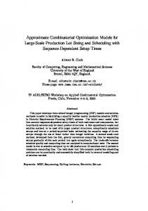
2.1.2. Edge-based methods The above presented region-based methods assume that the intensities inside a segment can be described in some uniform way. In practice these intensities can differ very much even if the object of interest has uniform color and reflectance properties on its entire surface. Such an object is the rabbit in Figure 2.3 (left). Yet, due to lighting effects the recorded intensities vary from dark to light. One would need a sophisticated probability distribution to describe these intensities, and this induces the problem of estimating its parameters. There is an alternative way to characterize segments which naturally handles lighting effects: it is based on the observation that object boundaries usually coincide with significant
30
2.1. Introduction to Image Segmentation brightness changes, i.e. they are located in places of high image gradients, called edges. More precisely, edges are oriented entities and perpendicular to the direction of steepest brightness change. Figure 2.3 (right) visualizes the location of edges for the input image on the left. More precisely it displays the output of the edge detector function g(x) =
δ , δ + |∇I(x)|
(2.3)
where δ is chosen as 30. Values near 0 appear in black, values near 1 in white. The figure clearly shows that many parts of the silhouette of the rabbit correspond to black regions indicating image edges. It also shows the two major challenges for the edge-based approach: firstly, some parts of the silhouette correspond to places of low contrast, called gaps, where no edges are detected. Secondly, not all places of high image gradients correspond to object boundaries. A powerful segmentation method must hence be able to close gaps as well as select the appropriate edges. As will be detailed below, suitable regularity terms for gap closure include the curvature of the region boundary. An experimental comparison of region-based and edge-based methods is deferred to Section 2.9.3 where the edge-based method proposed in this chapter is compared (among others) to the piecewise constant functional of Mumford and Shah. The Classical Approach: Line Integrals The classical approach to edge-based image segmentation is based on line integrals. These approaches assume that there is a single simply-connected foreground region, where the respective region boundary is denoted C : S1 → R2 . The discussion here relies on the notation introduced in Chapter 1.3.2. A very popular approach was given by Caselles et al. [36] and Kichenassamy et al. [125] who propose to minimize the integral of some positive edge detector function g : Ω → R+ along the region boundary: E(C) =
Z
S1
g(C(t)) |Ct (t)| dt .
(2.4)
The function g must assign low values to high image gradients and can e.g. be chosen as (2.3). The problem with (2.4) is that its minimum is the empty set (or, if the empty set is excluded, a curve that reduces to a point). The task becomes meaningful if a user provides so-called seed points, i.e. a set of points which are definitely foreground and a set of points which are definitely background. The arising problem, which is now a supervised one, can then be solved globally [24]. A precursor method of (2.4) is the famous snakes model that was introduced by Kass et al. [123] in 1988. They proposed to minimize the criterion E(C) = −
Z1 0
2
|∇I(C(t))| dt + α
Z1 0
2
|Ct (t)| dt + β
Z1 0
|Ctt (t)|2 dt ,
(2.5)
with weighting parameters α, β ≥ 0 and where no assumptions on the parameterization of C are given. This functional is not invariant to parameterization, which makes it hard to
31
2. Curvature in Image Segmentation understand and analyze. Kass et al. probably chose this form because it behaves favorably when evolving explicit (i.e. control point-based) parameterizations of the curve. From today’s perspective one would want a parameterization-invariant formulation which might read like this: Z Z E(C) = − |∇I(C(t))|2 |Ct (t)| dt + νkCk + λ |κC (t)|2 |Ct (t)| dt . (2.6) S1
S1
This criterion favors curves that are located at image edges. With length regularity alone the global minimum would – depending on ν – either not exist (curves would grow infinitely) or be the empty set. When also the curvature prior is active the global minimum can be meaningful when choosing suitable weights λ, ν > 0. Later on in this chapter we present a method that allows to identify – for each image individually – weights corresponding to meaningful global optima as well as compute a corresponding minimum. Minimizing Line Integrals The above given edge-based criteria have traditionally been minimized locally using gradient descent. Both explicit [123] and implicit [36] curve evolution methods have been used. In this field also global minimization methods are known and in fact they appeared quite early: in 1990 Amini et al. [5] showed how to optimize a modified snakes functional via distance calculations in graphs. Yet, their method has very high run-time demands and was therefore only applied to rather small search spaces. The method proposed in this chapter uses an algorithm proposed by Lawler [141] that allows large search areas in practice and was introduced to computer vision by Jermyn and Ishikawa [117]. The latter work is discussed in the section on hybrid methods below. Details on the optimization algorithm are presented in conjunction with the novelty later on in this chapter. Refined Edge-based Methods Many more edge-based methods have been proposed. One line of work is based on force fields, where an early work is given by the generalized gradient vector flow of Xu and Prince [211]. Jalba et al. [115] mimic the notion of electrostatic forces, Xie and Mirmehdi [210] instead use magnetostatic forces. The arising functionals are minimized via curve evolution and the results are often comparable to those produced by region-based methods. Another line of work addresses ratio functionals. Many of these works can also integrate region terms and are discussed in the subsequent section. A purely edge-based approach is given by the normalized cuts of Shi and Malik [191], which extends to an arbitrary number of segments. The underlying optimization problem is NP-hard. Using relaxation-techniques a solution is obtained that does not depend on initialization.
2.1.3. Hybrid Methods A number of methods exist to combine region-based and edge-based methods. A popular approach (e.g. [27, 175]) is to combine a region-based data term with a weighted length regularity term. For example, the respective adaptation of the piecewise constant MumfordShah functional (2.2) would be E(l, {µj }) =
32
Z �
Ω
I(x) − µl(x)
�2
Z
dx + ν g(s) ds , C
2.1. Introduction to Image Segmentation where g(·) could be the edge detector in (2.3). A very different line of work combines edge-based terms with region integrals inside the foreground region only. These methods are based on ratio functionals. Cox et al. [49] propose a method which is limited to planar graphs and results in quadratic run-times. A more general and efficient method was given by Jermyn and Ishikawa [117]. They address the minimization of a class of functionals of the form R
S1
v(C(t)) · nC (t) |Ct (t)| dt R
S1
g(C(t)) |Ct (t)| dt
,
(2.7)
with g(·) as before. Here v : R2 → R2 is a vector field (e.g. the image gradient), nC (t) is the unit curve normal3 of C at the point C(t) and “·” denotes the scalar product. Although (2.7) looks like a purely edge-based approach, it can easily include integrals over the region Cin enclosed by the contour. To this end, given a function f : R2 → R one constructs a vector field vf : R2 → R2 vf (x, y) =
1 2
�Z
x
f (t, y) dt
Z
y
f (x, t) dt
0
0
�⊤
.
(2.8)
From the Gauss-Green theorem it then follows that the respective numerator term in (2.7) is equal to the integral of f in the region Cin : Z
S1
vf (C(t)) · nC (t) |Ct (t)| dt =
Z
f (x) dx .
Cin
For further details see e.g. [117] and section 2.5. A very prominent member of the class (2.7) is the average outward flux, which will be studied in detail in this chapter: R
S1
∇I(C(t)) · nC (t) |Ct (t)| dt kCk
.
(2.9)
The numerator of this functional is known as flux. It is typically employed when long and thin structures are to be segmented [202, 132]. In the context of (2.9) it is important that the functional is optimized over oriented curves, i.e. traversing the curve in clockwise direction is different from a counter-clockwise traversal: when changing the direction of traversal, all normals change sign and so does the entire numerator term. This implies a negative minimum and that minimization is equivalent to maximizing the absolute of the ratio: min C
= max C
3
R
S1
∇I(C(t)) · nC (t) |Ct (t)| dt kCk
R ∇I(C(t)) · nC (t) |Ct (t)| dt S1
kCk
.
It is obtained by rotating the normalized first derivative vector clock-wise by 90 degrees.
33
2. Curvature in Image Segmentation
well handled by average flux (background darker than foreground).
not well handled by average flux (background partially lighter and partially darker than foreground).
Figure 2.4.: The average outward flux (2.9) requires that the foreground is either consistently darker or consistently lighter than the background. (The resulting globally optimal contours are shown in yellow). This optimization task therefore favors curves that coincide both with the location and the orientation of image edges. Since the absolute is outside the integral it also requires that the enclosed foreground area is consistently lighter or consistently darker than the background. That is why the left image in Figure 2.4 is segmented correctly. In contrast, the right image is not treated as one would desire: here the foreground is partially lighter and partially darker than the background. The numerator terms will then cancel out and the result is near zero.
2.2. Curvature and Computer Vision Problems The novelty of this chapter is to extend the class of functionals (2.7) to include curvature regularity. Kanizsa [122] showed that curvature plays an important role in human scene interpretation. Not surprisingly, it is regarded as a powerful prior in many areas of computer vision. RIts first appearance was in the context of shape completion through Euler’s elastica energy 01 |κC (t)|2 |Ct (t)| dt, see [201, 109, 157] and the more recent works [190, 127, 80, 44]. Relevant application areas include image segmentation [123, 5, 161, 75], inpainting [8, 40, 151, 77, 78], image smoothing and denoising (see [199] and references in [35]) and image analysis [166, 74]. Minimizing curvature-based functionals is an intricate problem which has traditionally been addressed by local curve evolution. Apart from the heavy dependence on an initialization, here one also has to deal with fourth-order derivatives in the gradient descent process. The calculation of these derivatives is numerically unstable and prone to errors due to noise. A recent line of work, started by Grzibovskis and Heintz [101] and continued by Esedoglu et al. [76], manages to perform curve evolution by using only second-order derivatives. To be precise, the correct gradient flow is approximated by combining second-order derivatives with Gaussian convolutions. In the context of inpainting Masnou and Morel [152, 151] are able to optimize absolute curvature globally for completing level lines. If also data terms are included in the functional, global solutions are available when minimizing discrete versions of the functionals. The convergence of such processes was considered by Bruckstein et al. [33]. The underlying discrete algorithms are based on product graphs,
34
2.3. Contribution where each node in the graph represents an image pixel and an incoming direction. Details will be given in conjunction with the contribution of this chapter. Amini et al. [5, 4] apply distance calculations in graphs to obtain global minima. Parent and Zucker [166] independently exploit the same product space, but in a context that does not admit global solutions.
2.3. Contribution The contribution of this chapter is the extension of the class (2.7) of globally optimizable ratio functionals to include curvature regularity. The proposed method is very general as it allows almost arbitrary functional dependences of the integrands on location, tangent angle and curvature. This is achieved by combining the graph-based ratio minimization algorithm used in [117] with the product graph used for curvature. Ways to efficiently handle the rather large graphs are presented. It will be shown that the proposed method gives rise to substantially larger regions than the average outward flux (2.9): curvature is an important prior to deal with gap closure. The method also compares favorably to region-based methods. Lastly, the proposed method can be used to find parameter sets where the parameterizationinvariant re-formulation (2.6) of the snakes functional has a meaningful global optimum. In fact, such an optimum is output simultaneously. This is joint work with Simon Masnou and Daniel Cremers. A short version was published in [182], an extended version has been submitted to a journal.
2.4. Introducing Curvature into Ratio Optimization Above we have met the average outward flux, which amounts to the optimization task
max C
R ∇I(C(t)) · nC (t) |Ct (t)| dt S1
kCk
.
While this gives meaningful global optima – the optimum is neither a single point nor an infinitely long curve – in practice the results do not correlate well with human perception. The functional often favors small homogeneous regions that do not correspond to objects. As a remedy, Jermyn and Ishikawa propose to integrate a balloon force, i.e. a term favoring large areas enclosed by the curve. The resulting ratio functional is termed balloon ratio in this work: max C
R R ∇I(C(t)) · nC (t) |Ct (t)| dt ± β dx S1 Cin
kCk
,
(2.10)
where β ≥ 0 is the area weight and ± means to take the sign which gives the higher energy. The novel term is included via the Gauss-Green theorem as explained above. While this significantly improves the results, adjusting the area weight β seems a non-trivial issue. In particular, when choosing β too high one will get the entire image. This chapter proposes another way to deal with the problem: the inclusion of curvature into the average outward flux. Specifically, the problem of minimizing the elastic ratio
35
2. Curvature in Image Segmentation
input.
length-based.
curvature-based.
input.
length-based.
curvature-based.
Figure 2.5.: Effects of length-based and curvature-based regularization in image segmentation on artificial images. Compared are the average outward flux (2.9) and the elastic ratio without length regularity (ν = 0, q = 1). Note that curvature regularity allows to find larger regions and establishes gap completion.
min C
R
S1
∇I(C(t)) · nC (t) |Ct (t)| dt
νkCk +
R
S1
=
|κC (t)|q |Ct (t)| dt
(2.11)
R ∇I(C(t)) · nC (t) |Ct (t)| dt S1 R max q C
νkCk +
S1
|κC (t)| |Ct (t)| dt
is addressed, where the denominator is now a weighted combination (with weighting parameter ν ≥ 0) of length and some power q > 0 of absolute curvature. Figure 2.5 shows the effect of curvature in this functional - it compares a result without length (i.e. ν = 0) to the average outward flux. Clearly curvature-regularity allows gap closure, whereas length-based regularity does not. The reason is that curvature only penalizes direction changes. Hence, if the curve contains a straight line, the curvature term will not contribute. At the same time, the data terms will accumulate, so the ratio can grow. This is not possible using length regularity since this induces cost for every part of the curve. For practical images it proves best to combine length and curvature regularity. In fact, the proposed method can handle a much wider class of functionals: it can optimize the ratio of two line integrals where the integrands in numerator and denominator can have almost arbitrary dependences on the position C(t), tangent angle αC (t) and curvature κC (t) of the curve. The supported functionals are of the form
36
2.5. The Problem with Region Terms
f(x) = 1
f(x) = -1
Figure 2.6.: The trouble with self-intersecting curves: the considered algorithm provides curve normals nC (shown in blue) that are partially inner normals and partially outer ones. With these normals, the left-hand side of (2.1.3) evaluates the region integral as ±2, whereas the right-hand side gives the correct value of 0. R
S1
h(C(t), αC (t), κC (t)) |Ct (t)| dt
S1
g(C(t), αC (t), κC (t)) |Ct (t)| dt
min R C
,
(2.12)
with functions h, g : R2 × [0, 2π] × R → R and where the only requirement is that the denominator integral be strictly positive for all closed curves C. Before details on the method are given, we briefly describe why the above class does not include region terms.
2.5. The Problem with Region Terms The integration of region terms via the Gauss-Green theorem is not as straightforward as it may seem. The method we will use optimizes over any kind of curve, including self-intersecting ones. It also always estimates the curve normal as a clock-wise 90◦ -rotation of the normalized first derivative vector Ct (t). As visualized in Figure 2.6, for a self-intersecting curve a part of the curve normals point inside the enclosed area, the other part point outside of it. Yet, to correctly apply the GaussGreen theorem, one needs consistent normals, e.g. all pointing inwards. As a consequence, self-intersecting curves are not assigned the desired cost and in fact a modified optimization problem is solved. One needs to make sure that all global optimizers of this modified problem are non-self-intersecting curves. Otherwise the procedure becomes meaningless. For the balloon ratio (2.10) this property is indeed given. Still, in general it is a non-trivial design problem to find suitable functionals. For this reason region terms will not be treated in the remainder of this chapter.
2.6. Minimizing Curvature Ratios Having detailed the problem statements, we will now turn to the question of how to minimize the respective functionals. The problems (2.11) and (2.12) are continuous optimization problems where the minimization is carried out over the space of all continuous curves S1 → Ω.
37
2. Curvature in Image Segmentation For such a continuous problem, the question of whether there exists a minimizer arises. More precisely, the question is whether the set {E(C) | C : S1 → Ω} has a minimum (i.e. a member of the set which is less than or equal to all other members of the set), where E(C) denotes the respective ratio of the curve C. For infinite sets this is generally not granted: for example, the set {x ∈ R | x > 0} does not have a minimum – one can get arbitrarily close to 0, but no matter what element one picks, there is always a smaller one. For the elastic ratio (2.11), under certain conditions it can indeed be shown that a minimizer exists. The proof as well as the conditions are given in Appendix A. Both are due to Simon Masnou. This proof also extends to the snakes ratio considered later in this chapter. For the general class (2.12) no results are known. Once it is clear that a minimizer exists one faces the question of how to compute it. Only few problems can be solved analytically and the elastic ratio is most likely not one of them. Hence, we are aiming at computer-based optimization tools which will require to discretize the problem in some form. This implies that the space of solutions will have to be restricted. One such restriction would be to consider the space of spline-functions (cf. e.g. [87, Chapter 11.2]) with either a fixed or a variable number of control points (see also [56] for a region-based task). This would still be a continuous optimization task. However, for this space we only know of local optimization methods, whereas we are aiming at a global one. Instead we will consider a discrete optimization task and restrict the set of valid curves to those having a polygonal form. To this end the image is discretized into pixels. Then a set of line segments connecting the pixel centers is set up. We take all line segments connecting points no more than a certain distance apart. The optimal curve can then be composed out of these line segments. The result is a discrete energy function which assigns a curve consisting of the line segments l1 , . . . , lP the energy P P
i=1 P P
n(li , li+1 ) ,
(2.13)
d(li , li+1 )
i=1
where wrap-around is used, i.e. P + 1 ≡ 1. The precise form of n(·, ·) and d(·, ·) is deferred to the subsequent sections where it will be shown that the problem can be optimized globally. Note that both n(·, ·) and d(·, ·) depend on pairs of line segments: it is not possible to estimate curvature from a single line segment. This approach raises the question of how well the discretized problem reflects the continuous one. Before we discuss this, however, the method is described in greater detail.
2.7. The Optimal Contour as a Cycle in a Graph To optimize the discretized problem (2.13), it is mapped to the problem of finding an optimal cycle in a graph. Such a cycle will be found via Lawler’s ratio cycle algorithm [141]. The standard approach to setting up a graph would be to assign a node to each image pixel and an edge to each possible line segment. Yet, Lawler’s algorithm can only handle functionals of
38
2.7. The Optimal Contour as a Cycle in a Graph the form
P
n(e)
e∈Γ
min P Γ
d(e)
,
(2.14)
e∈Γ
where each e is an edge in the graph and Γ is a cycle. Using the described graph, weights depending on pairs of edges would be required. As observed by Amini et al. [5] a graph where curvature-based weights correspond to single edges is easily constructed by reverting to a product space: a node now represents a line segment, i.e. a pair of image pixels instead of a single image pixel. That is, the node set is now of the form V = { (x1 , x2 ) | 0 < |x1 − x2 | ≤ R } , where R is a pre-specified limit on the length of the maximal line segment. Edges in the graph connect line segments that may follow each other, i.e. that share a pixel: E = { (x1 , x2 ), (x2 , x3 ) ∈ V 2 } . �
Using these edges, the discrete objective function (2.13) is easily brought to the form (2.14). We can now turn to the question of how the edge weights n(e) and d(e) are defined.
2.7.1. Estimating Curvature, Normals and Tangent Angles The considered class of functionals allows dependences on tangent angles and curvature. Hence, for each edge these quantities have to be estimated. The curve normals can either be derived from the tangent angle or by normalizing the vector x2 − x1 and rotating it by 90◦ . Tangent angles and normals are calculated for each line segment individually. Hence, as an edge represents two line segments, it is assigned two angles and normals. The tangent angle is given by the angle of the difference vector x2 − x1 . This angle can be computed by the function atan(·) and a case distinction which may add an angle of π. Since this calculation is comprised in the standard C++-function atan2, the equation is omitted here. To estimate the curvature, one needs to look at both line segments at once. To obtain optimal convergence properties, we follow the result of Bruckstein et al. [33] and define the absolute curvature of an edge as |κ|(x1 , x2 , x3 ) =
1 2
|α1,2 − α2,3 |S1 , min(|x2 − x1 |, |x3 − x2 |)
(2.15)
where α1,2 and α2,3 are the tangent angles of the respective line segments. The index S1 on the absolute indicates that the distance on the manifold S1 is taken, i.e. the jump over 2π is correctly accounted for.
2.7.2. Setting up the Edge Weights For the elastic ratio (2.11) (and also the snakes ratio presented later on) we use tailor-suited edge weights. For the numerator we discretize each line segment via the method of Bresenham [28]. Then we evaluate the data term for each pixel using the above mentioned segment normal and sum the obtained values. For the denominator we evaluate length-based and curvature-based terms separately. For the length term, each edge represents the length of the second line segment. For the curvature
39
2. Curvature in Image Segmentation Minimum Ratio Cycle Algorithm Input: A graph G = (V, E) with two edges weights n(e) and d(e) for each edge. A root node r ∈ V. P P Output: A cycle Γ reachable from r which minimizes the ratio e∈Γ n(e)/ e∈Γ d(e) among all such cycles. 1. Find an upper bound λ on the optimal ratio λopt . 2. Compute edge weights w(e) = n(e) − λd(e) for each edge e ∈ E. 3. Call the Moore-Bellman-Ford algorithm (Fig. 2.8) for the graph G with root node r and the edge weights w. If it returns a negative cycle, set λ to its ratio and go to 2. Otherwise output the last found cycle and stop.
Figure 2.7.: Ratio optimization after Lawler [141]. Shown is the linear search variant, also known as Dinkelbach’s method [66]. term we evaluate the expression (2.15) and take the desired power of it. Finally, to get the integral of this term, the length of the segment needs to be included in the weights. Here again we follow the results of [33] and assign the edge the quantity 1 2
min(|x2 − x1 |, |x3 − x2 |) · [|κ|(x1 , x2 , x3 )]q .
for the integral of curvature. In the general case (2.12) things become more difficult: e.g. one has to handle terms like R 1 S I(C(t)) |κC (t)| |Ct (t)| dt where the integrand depends both on position and on curvature. This makes it much harder to reflect the continuous functional in terms of discrete sums. Our solution is presently to calculate the Bresenham lines, then calculate the values of h(·, ·, ·) and g(·, ·, ·) for each pixel, using the above given estimates for normals and curvature. These values are then summed to form the edge weights.
2.7.3. Convergence of the Process We now know the exact form of the discrete functional that is optimized globally. So far we assumed a fixed pixel grid, say with pixels of size h × h and a given radius R defining the maximal length of line segments. One can now consider what happens if the number of pixels is increased, i.e. if h tends to zero (h → 0). It turns out that in this case a sequence of discrete global optimizers does indeed converge to a global optimizer of the continuous problem. In fact one can even decrease the radius R to h R. A prove is given in Appendix B. It is due to Simon Masnou and also extends to the snakes ratio considered later on.
2.8. Ratio Optimization over Cycles in a Graph Having set up the graph and its edge weights, it remains to find a globally optimal cycle in the graph. To this end we use a variant of the Minimum Ratio Cycle algorithm proposed
40
2.8. Ratio Optimization over Cycles in a Graph by Lawler [141, 59]: instead of binary search we use linear search as proposed by Dinkelbach [66], which is much faster in practice. This section also discusses efficient implementations on sequential and parallel architectures. Recall that the task is to minimize the function P
n(e)
e∈Γ
min P Γ
d(e)
e∈Γ
over all cycles Γ in the graph, where the sum over d(e) must be positive for all cycles. For the practical implementation we also use quantized weights n(e) and d(e) and represent them as integers. This point is crucial to get a polynomial time complexity. To obtain convergence to the continuous problem, the level of quantization needs to be refined as well. The basic algorithm is shown in Figure 2.7. It is based on iterated negative cycle detection in a graph with single edge weights. To see why this works, let λ be some ratio and define edge weights w(e) = n(e) − λ d(e) . Now suppose the graph contains a negative cycle Γ w.r.t. the edge weights w(e). By applying equivalence transformations one sees that any such cycle must be of a better ratio than λ and vice versa: X
w(e) < 0
e∈Γ
⇔ ⇔ ⇔
X
[n(e) − λ d(e)] < 0
e∈Γ
X
n(e) < λ
e∈Γ
X
d(e)
e∈Γ
P n(e) Pe∈Γ 0 be the level of quantization (i.e. all weights are multiples of ǫ), wn be the maximum absolute numerator weight and wd the maximum absolute denominator weight, both before quantization. One can show [117] that the number of calls is then O(m3 wd2 wn /ǫ3 ) in the worst case, with m the number of edges. In practice the number of iterations is less
43
2. Curvature in Image Segmentation
segmentations obtained with the average outward flux.
segmentations obtained with the elastic ratio.
Figure 2.9.: The elastic ratio gives rise to more meaningful segmentations than the average outward flux. In particular, it is able to find objects in the presence of partially low contrast. than 50 for ǫ = 10−3 and a radius R = 3. This was checked on a wide variety of images consisting of up to 640 × 480 pixels. In total this results in the rather high run-time complexity of O(|P|5 R18 wd2 wn /ǫ3 ). Note that this is just an upper bound on the run-time. It may be possible to prove tighter bounds. Also, for practicable problem instances a linear dependence on the number of image pixels is observed. On the GPU, even images of size 640 × 480 are processed in less than half an hour, again for a radius of R = 3.
2.9. Experiments for the Elastic Ratio We will now present results for the elastic ratio (2.11) on practical segmentation tasks. In particular, these results will demonstrate the following points: • The elastic ratio with squared curvature allows object segmentation for a large variety of domains. The length weight ν was adjusted experimentally on a variety of images. We found a value of 0.15 to give reliable results. • The functional is in fact robust to the choice of the length weight: for a broad range of parameters comparable results are obtained. • The proposed fully unsupervised method is able to outperform region-based methods in certain cases: it is less sensitive to shading effects, so it can find more precise boundaries. • Our method is robust to noise, i.e. even for very noisy pictures it produces results comparable to those on noise-free pictures. We emphasize that there is no need to adjust any parameters.
2.9.1. Average Flux vs. Elastic Ratio Figure 2.9 shows a comparison of ratio functionals on images containing objects in front of a cluttered background. In two cases the average outward flux finds a meaningful object: here
44
2.9. Experiments for the Elastic Ratio
segmentations obtained with the average outward flux.
segmentations obtained with the elastic ratio.
Figure 2.10.: The results on the Berkeley database confirm: the elastic ratio is better suited for object segmentation than the average outward flux. the entire object boundary has a high contrast. On these images the elastic ratio produces comparable results. In the majority of cases, however, the average outward flux favors small homogeneous regions. The figure shows that in many of these cases the elastic ratio is able to locate meaningful objects. This trend is confirmed by Figure 2.10, where we show some results on the Berkeley database. To find larger regions, Jermyn and Ishikawa [117] revert to the balloon ratio (2.10) which includes a suitably weighted balloon force. Figure 2.116 demonstrates that there are fairly large parameter ranges which give rise to almost identical segmentations. The functional therefore seems robust to the choice of the area weight. However, there is no parameter that works well for all the shown images. Nonetheless the balloon ratio produces meaningful objects in several cases and we consider it somewhat complementary to the elastic ratio: each gives rise to segmentations that cannot be produced with the respective other one. In general, whether one wants to favor objects with a large area or with low curvature of the region boundary will depend on the application.
2.9.2. Efficiency on CPU and GPU Due to the large search space an efficient procedure for minimizing the elastic ratio is desirable. Consequently, the underlying combinatorial algorithm was implemented both on the CPU and on the GPU as described in Section 2.8. This section presents an evaluation of how the optimization process reacts to the different architectures. The ratio is initialized with 0 in both cases. The experiments were run on a Core2 Duo machine with 2.66 Ghz, where only a single core was used. The machine is furthermore equipped with 4 gigabyte of main memory and a GTX 8800 graphics card. The resulting run-times for several images are given in Table 2.1. For the smallest image the explicit graph uses roughly half the system memory. Here the explicit storage of edges 6
Many thanks to Greg Mori for sharing his data with us.
45
2. Curvature in Image Segmentation
The average outward flux usually identifies small homogeneous regions.
β = 0.8
β ∈ [0.71, 0.88]
β ∈ [0.9, 1.4]
β ∈ [0.9, 1.85]
β = 1.2
β = 1.375
β ∈ [1.25, 1.4] β ∈ [1.38, 1.55]
β = 0.9
β ∈ [1, 1.9]
β = 1.41 β = 1.9 β = 1.45 β = 1.56 β = 1.925 With a suitable area weight (±β), the balloon ratio finds meaningful regions.
The elastic ratio can identify body parts.
Figure 2.11.: Where the elastic ratio identifies body parts, the average outward flux only finds small homogeneous regions. With a suitable area weight the balloon ratio can find meaningful regions.
46
2.9. Experiments for the Elastic Ratio Image
Run-time
Name
Resolution
CPU-expl.
CPU-impl.
GPU
Seal
200 × 133
364s
812s
35s
Bunny
260 × 180
1567s
1593s
101s
Berkeley #3
321 × 481
N/A
8673s
1046s
Baseball #2
450 × 314
N/A
14810s
151s
Table 2.1.: Comparison of run-times for the different implementations. For the CPU runtimes with explicit storage of edges and with on-the-fly computation are shown. Experiments were run on the same machine and using compiler optimization. is about twice as fast as the implicit one – both on the CPU. For the second image the two perform almost identically: here the entire system memory of 4 GB was needed for explicit storage. The speed-up of the GPU version over the CPU one with implicit storage varies from a factor of 8 to a factor of 100. The huge deviations are due to7 the different natures of the algorithms (queue-based vs. full parallel). In particular, these differences result in a different sequence of intermediate ratios since the Moore-Bellman-Ford algorithm merely outputs some negative cycle, not the most negative one. All given run-times are quite high and often exceed half a minute. However, one should bear in mind that it is a fully unsupervised algorithm which still allows to separate the objects from the background.
2.9.3. Robustness and Comparison to Region-based Approaches For a comparison to region-based approaches two variants of Mumford-Shah-like functionals [158]8 were implemented: E(u1 , u2 , {ΩI }) =
X
i=1,2
Z
Ω
!
(I(x)−ui (x))2 1Ωi (x) + λ|∇ui (x)|2 dx + ν|∂Ωi | . σI2
(2.16)
Here a piecewise smooth approximation by two functions u1 , u2 : Ω → R and a partition of the image plane Ω into two disjoint regions Ω1 and Ω2 is computed by alternating globally optimal updates for ui and Ωi . The data fidelity terms – normalized with respect to the intensity variance σI2 – are only imposed in the regions indicated by the characteristic functions 1Ωi associated with region Ωi , and |∂Ωi | denotes the Euclidean boundary length of Ωi . The update with respect to ui (for fixed Ωi ) is obtained by solving the Euler-Lagrange equations (I −ui ) 1Ωi + λ σI2 ∆ui = 0 ,
i = 1, 2 ,
(2.17)
using Successive Over-Relaxation (SOR). The update of the regions Ωi for fixed ui can be computed in a globally optimal manner for a discrete approximation on a regular grid using 7 8
Also, we are using generic classes on the CPU, but specific code on the GPU. Note that functional (2.16) is not identical with the original Mumford-Shah approach since the smoothness terms in expression (2.16) are extended into the entire domain Ω.
47
2. Curvature in Image Segmentation
ν = 10−6
ν = 10−5
ν = 5 · 10−5
local minimizers (see text) of the piecewise constant Mumford-Shah.
ν = 0.0001
ν = 0.0005
ν = 0.0015
local minimizers (see text) of the piecewise smooth approximation.
global optimum of the elastic ratio.
Figure 2.12.: The elastic ratio extracts the object almost perfectly. Moreover it is robust to noise, without the need to change any parameters. In contrast, both the piecewise constant Mumford-Shah [158] and the piecewise smooth approximations (α = 5 · 10−5 ) fail to differentiate the object from the background and are more sensitive to noise.
48
2.10. A Connection to the Snakes Model
ν = 0.01
ν = 0.05
ν = 0.25
ν = 0.3
ν = 0.5
ν = 0.75
ν=1
ν = 0.01
ν = 0.05
ν = 0.25
ν = 0.3
ν = 0.5
ν = 0.75
ν=1
Figure 2.13.: Effect of the length weight on the elastic ratio: for a fairly large parameter range a meaningful part of the image is found. graph cuts [22]9 . For λ → ∞ one obtains piecewise constant approximations with scalar constants ui given by the mean gray value in region Ωi . The performances of the elastic ratio and (2.16) are compared in Figure 2.12. Already for the noise-free image we could not find a length parameter where the Mumford-Shahtype implementation separates the object from the background. For the highly noisy images, despite the adaptive smoothness terms numerous small regions arise. In contrast, the elastic ratio identifies the object almost perfectly without needing to adjust any parameters. Lastly we address the robustness of the elastic ratio with respect to the length weight ν. Figure 2.13 demonstrates that for a fairly large range of ν the object is found. Up to a certain point the contour becomes more complex with increasing ν. From this point on the length term becomes dominant and the functional approaches the average outward flux.
2.10. A Connection to the Snakes Model The presented method allows to draw conclusions about the parameterization-invariant reformulation of the snakes model (2.6) which is restated here for convenience in a slight variation: E(C) = −
Z
S1
Z
|∇I(C(t))|p |Ct (t)| dt + νλkCk + λ |κC (t)|q |Ct (t)| dt .
(2.18)
S1
Two things have changed here: firstly, we introduced parameters p, q ≥ 0 for the powers of absolute image gradient and curvature. Secondly, the parameters λ and ν are now multiplied to form the weight of the length term. The mentioned connection is based on a relation of ratio optimization to parameter selection. This connection is discussed in this section, and the implications are demonstrated experimentally. 9
A related efficient algorithm for minimizing the piecewise smooth Mumford Shah functional by alternating graph cuts and smooth approximations was independently developed by Grady and Alvino and evaluated in greater detail in [98].
49
2. Curvature in Image Segmentation
2.10.1. Parameter Selection via Ratio Optimization In Section 2.8 it was shown that Lawler’s algorithm minimizes a sequence of line integrals where a weighted version of the denominator is subtracted from the numerator. For the final line integral a global minimizer with energy 0 is found. This implies that minimizing a ratio allows to find a parameter setting where the associated line energy has a meaningful global optimum. Precisely this observation was made by Jermyn and Ishikawa in [117]. With the extended class of functionals introduced in this chapter one can now shed a light on the re-formulated snakes model (2.18). This is now explained in detail. To this end, consider what is termed the snakes ratio in this work: − E(C) =
Z
S1
|∇I(C(t))|p |Ct (t)| dt
νkCk +
R
S1
|κC (t)|q |Ct (t)| dt
,
(2.19)
where a parameter p for the influence of the image gradient was introduced. When applying Lawler’s algorithm to this ratio with p = q = 2, one ends up computing a negative optimal ratio λopt ≤ 0 and an optimal curve Copt so that −
Z
S1
2
|∇I(Copt (t))| |Ct (t)| dt + |λopt |νkCopt k + |λopt |
Z
S1
|κCopt (t)|2 |Ct (t)| dt = 0 ,
and no other curve has a smaller energy with respect to the same parameter |λopt |. Hence the snakes ratio provides valuable insights into the modified snakes model (2.18): given a relative weight ν between length and curvature regularity, minimizing the snakes ratio provides an absolute regularity weight |λopt | for which the parameterization-invariant snakes model (2.18) has a meaningful optimum and also the associated optimal curve. This means that now a model can be optimized globally for which previously only local solutions were available.
2.10.2. Experiments Due to computational issues (i.e. to be able to use integer optimization without causing overflows) we will state results for the snakes ratio with absolute image gradient (p = 1) only. The results with squared absolutes are unlikely to be better as places with low contrast are even more strongly disfavored than before. Figure 2.14 presents results on a variety of images. When using the balancing weight ν = 0.15 for length against curvature – which works well for the elastic ratio – the results are discouraging: in most cases the curve goes one way, turns around and takes almost exactly the same way back. This will not happen when using flux-based functionals: for the shown curves the numerator terms will cancel and the resulting near-zero energy will not be the globally optimal one. When reducing the influence of the length term (ν → 0) larger regions are found. For most images these regions are very close to convex and they usually do not correspond to meaningful objects. Since our algorithm always finds parameter sets where the global solution to the line energy (2.18) (now with p = 1) has the energy 0, one cannot draw conclusions about the entire functional. However, we consider it unlikely that other meaningful parameter sets lead to significantly better results.
50
2.11. Discussion
the snakes ratio (p = 1) with ν = 0.15.
the snakes ratio (p = 1) with ν = 0.01.
Figure 2.14.: The snakes ratio reveals: the gradient absolute is a bit weak as a data term.
2.11. Discussion This chapter has presented an edge-based approach for fully unsupervised image segmentation. It combines a product graph for minimizing curvature-based functionals with a model that guarantees meaningful global optima and an efficient algorithm to compute these optima. In practice it is fast enough to work also on large images. For moderately complex images the method is able to identify objects and due to its edgebased nature it excels in cases where region-based methods get confused. In these cases one even observes a strong robustness to the weight of length regularity in the objective function. It should be clarified, however, that region-based methods are applicable to a larger class of problems. In particular, they extend to an arbitrary number of segments, whereas the presented method can only find one region. Hence, for more complex images we recommend the use of region-based approaches. Still, a significant advantage of the presented contour-based approach is that it readily extends to the integration of shape knowledge while preserving global optimality – and with it the independence of initialization. Precisely this is the topic of the next chapter.
51
3. Shape Knowledge in Image Segmentation In the previous chapter we have dealt with the task of fully unsupervised image segmentation. We have presented a contour-based approach which integrates curvature regularity and hence establishes gap closure. In practice fully unsupervised methods are far from satisfactory: so far it has not been possible to capture the notions of human scene interpretation in a mathematically precise way. Moreover, humans heavily rely on prior knowledge: they actually interpret images instead of grouping brightnesses. Consequently, this chapter deals with the integration of shape knowledge into segmentation processes. The program will be given the outline (or contour / silhouette) of an object. The task is then to locate a – possibly deformed – equivalent of this contour in the image. This is achieved with translation invariance, i.e. the method does not rely on an initialization. Many methods require a set of training shapes to accurately model the deformation processes. In this chapter it will be shown that actually a single shape suffices. It presents two shape measures, the basic one allowing the contour to locally stretch and shrink and also to rotate globally. The refined model then also incorporates strong deformations by allowing parts of the shape to rotate locally. The chapter starts with an overview of related work, then proceeds to the presentation of the basic method. Subsequently, extensions to the tracking of objects and the handling of highly deformable shape measures are presented.
3.1. Related Work To study the related work, we will first cover the modeling aspects, then discuss the algorithmic side.
3.1.1. Prior Knowledge in Computer Vision State-of-the-art methods in computer vision allow to incorporate various levels of prior knowledge. High level methods introduce 3D-object models such as stick figures to model humans. The associated problem is known as pose estimation and is not covered in this work. In a simplified setting one does not care about the position of parts in 3D-space but only about their location in the image. These models are known as pictorial structures and date back to the work of Fischler and Elschlager [86]. They require a decomposition of the shape into meaningful parts. Recent publications include [84, 174]. This chapter focuses on methods that do not require an object model. The addressed methods are based on planar shapes which is abbreviated to “shapes” in the following. As illustrated in Figure 3.1, a (planar) shape is a binary image where the black parts indicate points that belong to the shape. There can be multiple disconnected regions and regions with holes.
52
3.1. Related Work
Figure 3.1.: Shapes are binary maps with black parts indicating points that belong to the shape. Here some shapes of walking persons are shown. (Data courtesy of ChanSu Lee and Ahmed Elgammal). This field is divided into methods that work with a single shape and those that require a set of training shapes. Methods requiring training shapes estimate the deformation characteristics of the shapes from the training data. This field was started by the seminal work of Grenander et al. [100] and refined by Cootes and Taylor [46]. Cremers et al. [56] model shapes via explicit contours and model the deformations of the control points. More recent works are based on the level set method, including works of Leventon et al. [144], Tsai et al. [198], Rousson and Paragios [177] and Cremers et al. [52]. Recently Cremers et al. [53] proposed a solution based on probability functions. Subsequently Lempitsky et al. [142] proposed a related method which requires substantially more training data. All of these methods rely on an area-based shape similarity measure which needs to preestimate the deformation characteristics of the shape from the training shapes. In contrast, a few methods exist which incorporate sophisticated shape measures based on point correspondences and work with a single shape template. So far all methods are limited to simply-connected shapes, i.e. shapes without holes. Felzenszwalb [83] models the shape via its Delaunay triangulation and allows deformations of the triangles. This allows to combine region-based deformation terms with edge-based data terms. The method is globally optimal and hence translation-invariant. In practice it requires to reduce the search space since otherwise the computational cost would be too high - see the paragraph on minimizing shape-based energies below. Coughlan et al. [48] locate an open contour (the outline of a shape) in an image and establish translation-invariance. This method allows to incorporate a sophisticated elastic shape similarity measure [148, 153] based on point correspondences and also allows to find multiple instances of the shape. It differs from all the above mentioned ones in that it does not perform segmentation – this is not possible with open contours. In [47] Coughlan and Ferreira give an extension to contours with holes.
3.1.2. Minimizing Shape-based Energy Functionals Traditionally shape-based energies have been minimized locally via contour evolution. This holds for almost all above mentioned methods requiring training sets. The employed paradigms are either explicit contour evolution [100, 46, 56] or level sets [144, 198, 177, 52]. These methods depend on initialization and require a careful adjustment of the numerical parameters used in the evolution processes. A very recent exception is the work of Cremers et al. [53] which allows to globally optimize in the space of probability functions and hence establishes translation-invariance. This
53
3. Shape Knowledge in Image Segmentation
inputs.
outputs.
Figure 3.2.: Starting from a prior contour and an input image, the proposed method simultaneously locates the (possibly deformed) contour in the image and computes a correspondence function between the two curves. (Image data courtesy of Bodo Rosenhahn.) method combines the estimation of deformation parameters with a Lipschitz search over translations. Subsequently Lempitsky et al. [142] proposed a combination of branch-and-bound and graph cuts for a model which does not involve deformation parameters. Methods based on single templates are more advanced. They allow global, translationinvariant solutions with sophisticated shape similarity measures. Felzenszwalb [83] uses dynamic programming in a special kind of graph (called chordal). Since the memory consumption of this method is quadratic, at present one cannot handle reasonably large images without previously reducing the search space. The method of Coughlan et al. [48] for locating open contours is also based on dynamic programming and allows global optima. It can be applied efficiently for very large images. Moreover, it is most closely related to the method presented in this chapter. The extension of Coughlan and Ferreira [47] loses the property of global optimality. With the help of belief propagation, the authors give a solution that does not depend on user initialization.
3.2. Contribution The main contribution of this chapter is an efficient procedure to handle closed contours for the problem of image segmentation with elastic shape priors. This problem is handled in a globally optimal manner. The memory consumption of the method is linear in the number of pixels and although the running time is a high order polynomial in the worst case, for practical problem instances a linear dependence is observed. The combination of all these properties allows the treatment of the entire image information during the optimization process. That
54
3.3. Outline of the Method is, there is no need to reduce the search space before optimization is started. Compared to the work of Coughlan et al. [48] there are three contributions: firstly, the proposed method addresses the computationally much harder case of closed contours, which is solved in a computational time that is effectively linear in the number of pixels and also linear in the number of template points. Secondly, the presented model is a ratio functional and therefore exhibits a lower bias towards short curves. Thirdly, the extension to a highly deformable shape model is presented. This is joint work with Daniel Cremers. The contributions were published in [181, 183, 185]. An extended version has been submitted to a journal.
3.3. Outline of the Method Figure 3.2 gives a rough overview of the presented algorithm: based on a single template only, the method simultaneously locates a deformed version of a closed input contour in the image and computes a matching between the two contours. It incorporates translation-invariance and optionally allows rotational invariance. The method is based on globally minimizing a ratio functional which incorporates a sophisticated elastic shape similarity measure [148, 153]. To this end, the problem is first mapped to optimizing over cycles in a product space spanned by the image and the template. By discretizing this space into a graph, the problem is ultimately mapped to finding the globally optimal cycle in a product graph. Such a cycle is found via an efficient combinatorial algorithm which gives an effectively linear dependence of the running times on the number of input pixels.
3.4. Combining Elastic Shape Priors and Image Segmentation Given is a prior contour, e.g. the outline of the pot in Figure 3.2, described by a curve S : S1 → R2 with a uniform parameterization. The task is to locate a (possibly deformed) equivalent of this contour in a given gray-scale image I : Ω → R – the extension to color images is straightforward. To this end, a contour C : S1 → Ω is determined which should be similar to the input contour and fulfill some data-driven criteria. In this work the contour is attracted by image edges. To allow deformations of the contour, a correspondence function is estimated. This orientation-preserving bijection is denoted m : S1 → S1 . It assigns each point on S a point on C and vice versa. This allows to use correspondence-based shape similarity measures which were shown to be important for reproducing human notions of shape similarity [93, 140]. The functions C and m can be combined into a single function Γ : S1 → Ω × S1 . This observation will be useful later when we discuss the optimization scheme. Before we present the employed functional, first the invariance to parameterizations is discussed.
3.4.1. Invariance to Parameterization For cost functions in computer vision invariance to the chosen parameterization is desirable. The presented cost functional is indeed invariant with respect to re-parameterizations of C.
55
3. Shape Knowledge in Image Segmentation C
g(x)
dS
1 C(t) (a)
|∇I(x)|
αC (t) dC
(b)
(c)
Figure 3.3.: The three ingredients of the proposed method: (a) an edge detector function assigning low values to high image gradients. (b) computation of tangent angles of the contours C and S (shown for C, the tangent is drawn in black). (c) computation of length distortion. It is not invariant to re-parameterizations of Γ : the reason is that the function m is not a stand-alone function – m(t) will always denote the correspondence of C(t). A change of the parameterization of C will therefore also entail a change in the parameterization of m. For this reason the functional is presented in terms of C and m rather than the combined function Γ. In later sections we will return to the Γ-notation.
3.4.2. Characterizing the Optimal Matching The optimal pair of contour C and matching m is characterized as the global minimum of a ratio energy. It combines three terms which are visualized in Figure 3.3 and now described in greater detail: 1. Data term. The employed data term aims at attracting the curve C to edges in the image. To this end, an edge detector function is used which assigns low cost to places of high image gradients. We use the function g(x) =
1 , 1 + |∇I(x)|
(3.1)
as shown in Figure 3.3a. Note that a variety of other functions could be used. In particular, the function is readily extended to handle color images. Integrating such a positive function along the contour C entails a strong bias towards short curves. To alleviate the problem the integral is normalized by the contour length, which results in averaging the edge detector function g(·) along the contour C: R
S1
g(C(t)) |Ct (t)| dt kCk
= < g >C ,
(3.2)
where < · > denotes the average. Shorter curves are still favored, but not as rigorously as before. The remaining bias is counteracted by the shape similarity measure. 2. Similarity of Curve Attributes. This is the first of two terms constituting the shape similarity measure. It performs a comparison of local attributes of corresponding points C(t) and S(m(t)). In this work – as shown in Figure 3.3b – the tangent angles of the curves are chosen as attributes. This implies translational invariance since translating
56
3.4. Combining Elastic Shape Priors and Image Segmentation a contour does not change its tangent angles. The integration of rotational invariance requires extra effort. This is deferred to Section 3.8.3. The similarity of corresponding tangent angles is measured by their squared cyclic difference |αC (t) − αS (m(t))|2S1 , where the difference is taken on the manifold S1 . Again we divide by the contour length and get the average deformation cost R αC (t) − αS (m(t)) 21 |Ct (t)| dt S
S1
kCk
=
Z
S1
αC (t) − αS (m(t)) 21 dt , S
(3.3)
where the second line holds for a uniform parameterization of C. 3. Penalties for Stretching and Shrinking. Aside from the monotonicity of the correspondence function, another regularity assumption is made: local stretching and shrinking of the contour is disfavored. The functional hence favors curves which preserve the scale of the prior contour. This counteracts the shrinking bias of the data term. In practice one observes a robustness with respect to gradual scale changes. The amount of stretching and shrinking is characterized as length distortion: consider Figure 3.3c where a piece dS of S corresponds to a piece dC of C, say at the point C(t). Then the length distortion is given by the quotient |dS|/|dC|. With a uniform parameterization of S this quotient can be expressed as1 kSk mt (t) |dS| (t) = . |dC| |Ct (t)| Recall that m is orientation-preserving, so without loss of generality its derivative is assumed to be positive. Numerous ways to penalize length distortion are conceivable. Before we present the chosen one, a few properties we consider essential for a penalty function are pointed out: a) A ratio of 1 (no distortion) should be assigned the penalty 0. b) As the ratio approaches ∞ (i.e. |dC| → 0 for fixed |dS|), so should the corresponding penalty. This point is crucial as the edge-based data term favors short curves and the shape attribute comparison is independent of scale. Hence, the penalty function must disfavor short curves. c) Preferably the shape similarity measure should be symmetric, i.e. comparing C to S should give the same cost as comparing S to C. This implies that the ratio |dS|/|dC| should be given the same penalty as its inverse |dC|/|dS|. The penalty function chosen in this work satisfies all three requirements: if K ≥ r ≥ 1 |dS| −1 = r − 1 if K1 ≤ r < 1 , Ψ r= |dC| ∞ otherwise �
1
�
r − 1
(3.4)
This term is indeed invariant against re-parameterization of C: any such re-parameterization will also change the correspondence function m and with it its derivative.
57
3. Shape Knowledge in Image Segmentation
Figure 3.4.: The structure of the product space Ω × S1 : for any point on the prior contour the space contains a copy of the image. A cycle (with winding number 1) then defines a contour as well as an assignment of any point on the contour to a point on the prior contour. Here K ∈ N+ is a predefined constant limiting the maximum length distortion. This limit will be exploited in the optimization algorithm. Like the two previous terms, the corresponding regularity term takes on the form of a ratio: R � kSk mt (t) � Ψ |Ct (t)| |Ct (t)| dt � Z � kSk mt (t) S1 R = Ψ dt , (3.5) |Ct (t)| dt |Ct (t)| S1
S1
where again equality holds for a uniform parameterization of C. This term is scaleinvariant in the sense that scaling both C and S by the same factor does not affect the cost. Using positive weighting factors λ, ν > 0 these terms are glued together into a single functional which is stated here for a uniform parameterization of C:
min
Γ=(C,m)
Z
S1
g(C(t)) dt + ν
Z
S1
� Z � αC (t) − αS (m(t)) 21 dt + λ Ψ kSk mt (t) dt S S1
kCk
(3.6)
The global minimization of a discrete version of this functional is now detailed. Note that the same scheme can be used for a variety of other functionals.
3.5. Optimization in a Product Graph The criterion (3.6) requires optimizing over functions of the form Γ : S1 → Ω × S1 .
58
3.5. Optimization in a Product Graph
6 7 8
4 5
3 2
1 9 0,|S|
Figure 3.5.: In the discrete problem, a shape is represented as a sequence of pixels on the image grid. Such functions are readily interpreted as cyclic paths (with winding number 1) in the threedimensional space Ω × S1 . This space is visualized in Figure 3.4: by multiplying a circle with the image domain, a space in the form of a torus arises. Hence, the problem can equivalently be stated as optimizing over cyclic paths in this torus space. A computer-based solution will require restricting the set of paths by applying a discretization. As in the previous chapter for curvature, we know of no method to globally optimize in a continuous space, e.g. the space of spline-functions. Instead, the space of admissible Γ-functions is restricted to those having a polygonal form. That is, the curve is now composed of line segments ∆Γ = (∆C, ∆m). These line segments are easily interpreted as edges in a graph with same topology as the product space shown in Figure 3.4. This way, the problem is reduced to finding the optimal cycle in a product graph, which is solved efficiently by applying Lawler’s minimal ratio cycle algorithm (cf. Chapter 2.8).
3.5.1. Discretizing Contours and Correspondences In addition to the cycle Γ also the prior contour S is discretized: it is represented as an ordered set of s0 , . . . s|S| of points on a suitable pixel grid, where – for ease of notation – s0 = s|S| is represented twice. To get a dense representation of the contour it is required that si be among the eight closest neighbors of si−1 . An example is shown in Figure 3.5. The curve pieces ∆C are chosen as straight lines connecting a pixel with one of its eight neighbors. The corresponding part ∆m of the correspondence function is also chosen as a linear function along ∆C. It is hence induced by its values at the start and end of ∆C. These values are indices in {0, . . . , |S|}. By design, i.e. since m is orientation-preserving, the index assigned to the end point of a line segment cannot be smaller than the one of its starting point. Both indices can however be equal. A First Attempt In the end the segments ∆Γ will be edges in a graph, so that again the functional can be represented via sums of edge weights. The problem is then reduced to finding the optimal cycle in the graph. In a first attempt one could introduce a node for each pair of image pixel and shape point, i.e. nodes of the form (x, i). The node set would then be P × {0, . . . , |S|} , where P is the set of image pixels. The problem with this approach is that very small cycles would arise: since several image pixels can be assigned to the same shape point, the graph
59
3. Shape Knowledge in Image Segmentation contains e.g. the cycle (x, i) → (y, i) → (x, i) where x and y are neighboring pixels. This – completely meaningless – cycle may well be the optimal cycle in the graph. Hence, a little more elaboration is needed. A Refined Graph Structure To circumvent this problem extra nodes are introduced. Now the first assignment of an image pixel to a shape point corresponds to a different state than its second assignment and so forth. To avoid an explosion in size, at this point it is exploited that the potential (3.4) limits the maximal amount of stretching and shrinking. In the discretization this is interpreted as a limit of K image pixels being associated to the same shape point. Hence the number of nodes increases only by a factor of K. The result is a graph with the node set P × {0, . . . , K · |S|} , where P is the set of image pixels. This set reflects that each shape point i can be assigned up to K image pixels. These K assignments are represented by the states i·K, . . . , i·K +(K −1). The edges in the graph are divided into two classes: in the first case, called type I edge, the start and end pixels of a line segment are assigned different shape points. These edges are of the form (type I) (x, i · K + k) → (y, j · K) with i < j ≤ i + K , where 0 ≤ i, j < |S| and 0 ≤ k < K are integers and x and y are neighboring pixels in the image. The set of all nodes with an index of i in the second component will be called the frame with the index i in the following. Edges of type II correspond to assigning both end points of the line segment to the same shape point. In this case one needs to keep track of the number of pixels already assigned to this shape point: (type II) (x, j · K + k) → (y, j · K + k + 1)
with k + 1 < K .
In this form the described graph is acyclic. However, recall that the shape points s0 and s|S| are actually identical. By merging the two states a cyclic graph is obtained2 .
3.5.2. Discretizing the Cost Function With the described graph structure, the cost functional (3.6) (and a large variety of other cost functionals) is easily brought to the discrete minimization problem P
n(e)
e∈Γ
min P Γ
d(e)
,
(3.7)
e∈Γ
where Γ denotes a cycle in a graph. The reader may recall that this problem already occurred in equation (2.14) in Chapter 2. Indeed the presented functionals are minimized using Lawler’s ratio cycle algorithm in combination with some extra effort. Before we come to the details, however, the edge weights n(e) and d(e) need to be set up. 2
This graph structure implies that shape point 0 cannot be skipped. Refined graphs without this property are conceivable, but require a more complex program structure.
60
3.5. Optimization in a Product Graph Since the denominator of (3.5) is merely the length of C, the denominator weights are given by |x − y|. The numerator weights are more intricate and require a distinction between type I and type II. It is however more convenient to state the contributions of each of the three terms in the cost functional separately: 1. Data term. For both types of edges, the data term contributes 1 |x − y| (g(x) + g(y)) . 2 2. Comparison of Tangent Angles. Let ϕ(x, y) be the tangent angle of the line segment connecting x and y. It can be computed via the function atan2 contained in most standard programming languages. The contribution of this term is then 2 ν |x − y| ϕ(x, y) − ϕ(sj−1 , sj ) S1 ,
again for edges of both types.
3. Length Distortion. A simple discretization of the length distortion penalty would be to add a term λ for type II edges and λ(j − i − 1) for type I edges. Both could further be multiplied with the length |x − y| of the segment. The problem with this discretization is that it assigns no cost when a diagonal line (of √ length 2) in the image is matched to a horizontal or vertical line (of length 1) in the prior template. We therefore now present a refined discretization which is closer to the continuous functional.
Type I Suppose the last aligned shape point was point i. For an edge of type I one either moves to the direct successor point j = i+1 or skips up to K−1 shape points. In both cases there can be length distortion. This distortion is computed as
|dS| = r= |dC|
j P
j ′ =i+1
|sj ′ − sj ′ −1 |
|x − y|
.
It is straightforward to compute the penalty by evaluating the function (3.4) on this term. In fact, for edges of type I one could use any other penalty function. Type II This case is more intricate since it implies that several line segments are matched to the same line sj−1 sj of the prior template. Here we will exploit the specific form of (3.4): once it is known that the length distortion ratio is below 1, the function is linear in r −1 − 1. Since all polygonal lines have a length of at least 1 and an edge of type I must already have been aligned to sj−1 sj , it is safe to exploit this for all type II edges. Let x0 x1 , . . . , xk−1 xk be all line segments of C aligned to sj−1 sj . Then the inverse ratio can be written as
r −1 =
k P
k ′ =1
|xk′ − xk′ −1 |
|sj − sj−1 |
=
k X |xk′ − xk′ −1 |
k ′ =1
|sj − sj−1 |
.
61
3. Shape Knowledge in Image Segmentation An edge of type II corresponds to only one of these line segments, e.g. x1 x2 , so the aim is to write the penalty for this ratio as a sum over the line segments. If the ratio for the segment x0 x1 is at least one, the type II edge can be given the penalty term λ
|x − y|2 . |sj − sj−1 |
The present implementation simply assumes that the first ratio is at least one. The only case where this assumption is violated is when x0 x1 is a horizontal or vertical line segment but sj−1 sj is a diagonal one. If one wants to handle this case correctly, the state space needs to be augmented. Type I edges with this property would then end in a new state. Type II edges leaving this state would be assigned a different length distortion cost.
3.6. Efficiently Minimizing the Discrete Problem At first glance one might be tempted to solve the discrete problem by applying Lawler’s ratio cycle algorithm as presented in Chapter 2.8. The problem is actually more intricate: by construction every polygonal Γ in the discretized search space corresponds to a cycle in the described graph. There are however cycles that do not correspond to a valid Γ: such cycles wrap around multiple times in the torus-graph3 . Hence, optimization needs to be restricted to the set of valid cycles that wrap around exactly once. This section first details how this restricted problem is solved, then proceeds to describe an efficient implementation.
3.6.1. Solving the Restricted Ratio Cycle Problem To solve the restricted problem, first Lawler’s ratio cycle algorithm is applied to all cycles in the graph. In most cases the computed optimal cycle is valid, i.e. wraps around exactly once. Yet, in about two percent of all cases an invalid cycle is found. In this case a recursive sub-division scheme is started: the set of nodes with the index 0 (i.e. all nodes of the form (x, 0)) is split into two parts. Then for each part Lawler’s algorithm is called for a graph where the respective other part has been removed – in practice the nodes are not removed but rather their distance labels are fixed to ∞. The initial ratio is set to the ratio of the last found valid cycle (or the original initial ratio if none was found). It is possible that a recursive call again finds an invalid cycle. In this case the respective part is again split into two parts and more recursive calls are made. To avoid useless calls one makes sure that the respective nodes with the index 0 in the found invalid cycle are not assigned to the same parts. In the end the best cycle among all parts forms an optimal cycle. In practice it is sensible to use an iterative implementation instead of a recursive one: this saves memory and allows to update the initial ratio during the process.
3.6.2. Efficient Memory Management The above presentation relies on a graph. Yet, due to the large search space standard pointerbased graph representations are not sensible: they would easily require terabytes of memory. This section presents a number of ways to reduce both the memory consumption and the running time. 3
In continuous terms: their winding number is two or higher.
62
3.6. Efficiently Minimizing the Discrete Problem
⇒
Figure 3.6.: The graph is cut open at frame 0 (shown in red) and the frame is doubled. The arising graph is acyclic. This is the key for efficient optimization. Implicit storage Recall from Section 2.8.1 that Lawler’s algorithm does not require an explicit storage of edges: it only maintains the distance labels of nodes. To keep the memory consumption bearable, the edges are therefore computed on-the-fly. The distance labels of the nodes are conveniently stored in matrices. In addition one needs to store predecessor entries for the best incoming edge for each node. These only need to code the number of the edge. For K ≤ 5 this can be encoded in one byte, otherwise two bytes are needed. Our current implementation uses four bytes. Sweep-based distance calculation To obtain further speed-ups we implement the distance calculation by a sequence of distance calculations on an acyclic graph: recall that the indices 0 and K · |S| were merged to form a cyclic graph. By reversing this process, an acyclic graph is obtained. That is, for all nodes with the index 0 a copy with the index K · |S| is introduced. All edges previously ending in frame 0 (i.e. the set of all nodes with the index 0) are connected to the respective nodes in the new frame. This is visualized in Figure 3.6. Now the distance calculation can be performed in sweeps. For the first sweep all distance labels in frame 0 are initialized with 0. Then in each sweep the distance labels and predecessor entries for the frames 1 to K · |S| are determined. Since the graph is acyclic and no edges connect nodes in the same frame, this can be done by dynamic programming. After each sweep the distance labels in frame 0 are compared to the respective ones in frame K · |S|. If the latter label is below the label in frame 0, this label and the corresponding predecessor entry are updated. In this case also the corresponding optimal path is extracted. If a (possibly invalid) cycle is found it must be a negative one (since the distance is negative and the initial distance 0) and the ratio is updated. Otherwise the ratio is kept and possibly another sweep has to be performed: this is the case if one of the distance labels in frame 0 was updated. In practice one seldom observes more than three sweeps for one ratio. Intermediate Storage The final storage-based improvement is less obvious but very important in practice. Before moving to the details it is useful to observe that at any time during a sweep one only needs to maintain a limited number of distance labels: the dynamic programming algorithm processes frames in the order of increasing indices. Since no edge skips more than K 2 frames, one only needs to keep track of the distance matrices for the previous K 2 frames. Less obvious, but quite important, is the observation that in fact only 2K instead of K 2 distance matrices need to be stored. Recall that edges of type I are of the form (p, i·K +k) →
63
3. Shape Knowledge in Image Segmentation (q, j · K). The important point is that the corresponding edge weights do not depend on k. In the distance calculation only the best of these K edges is needed. It corresponds to the optimal start node. This node must be computed only once for each shape point i and each pixel. Since the decision is needed for the following K shape points, this precomputation not only saves memory, but also yields considerable savings in run-time. By combining all these improvements, images of size 376 × 284 are processed with less than 750 megabyte.
3.6.3. Parallel Implementation In Chapter 2.8 it was stated that for general graphs Lawler’s algorithm is rather difficult to parallelize: on parallel platforms one cannot exploit list structures as are used to accelerate sequential implementations. For special kinds of graphs very efficient parallelizations do exist. The graph presented in this section is such a special graph. Recall that in the previous section an auxiliary acyclic graph was introduced. This graph has the nice property that edges never link two nodes in the same frame. The distances for an entire frame can therefore be determined in parallel. This was implemented on an NVidia GTX 280 graphics card with 240 parallel threads, using the CUDA framework4 . The running-times are reduced by a factor5 of about 16.
3.6.4. Profiting from Smart Initializations The final optimization aims at reducing the number of ratio adjustments in the ratio minimization process. In practice this number depends on the quality of the initial upper bound. If the prior contour fits entirely into the image, such a bound is easy to determine computationally: one can simply try several placements of the undeformed contour and calculate the respective ratios. Naturally, the number of placements needs to be balanced against the arising additional run time. In our experiments, optimal performance was achieved by trying displacements of up to 5 pixels in each direction around a central placement. Whenever possible this central placement is the one indicated by the user.
3.7. Complexity of the Method To analyze the worst-case running time of the method, let us first ignore the subdivision scheme and analyze a single call of Lawler’s algorithm. Each call of the Moore-Bellman-Ford algorithm has a complexity of O(|S|2 |P|2 ). The employed linear search scheme invokes at most O(|S|3 |P|3 wd2 wn /ǫ3 ) calls of the Moore-Bellman-Ford algorithm, where wn and wd are the maximal numerator and denominator weights before quantization and ǫ > 0 is the level of quantization (compare also Chapter 2.8.4). Finally, the recursive subdivision scheme makes O(|P|2 ) calls in the worst case. Together this results in a complexity of O(|S|5 |P|7 wd2 wn /ǫ3 ). As in the previous chapter, this is just an upper bound on the running time. It is possible that tighter bounds exist: after all, the given analysis holds for any kind of graph with the same number of edges and nodes and does not make assumptions on the cost function. 4 5
www.nvidia.com/cuda. In the conference paper [181] we erroneously reported a factor of 300. The confusion is probably due to an inappropriate choice of data structures in the CPU code used for [181].
64
3.8. Experiments for Image Segmentation
prior contour.
low contrast in input data.
matching after 3D-rotation.
shape deformation.
after stronger 3D-rotation.
shape deformation.
matching to another image sequence.
scale change.
Figure 3.7.: Translation-invariant matching of a contour to an image. The prior contour (red) undergoes significant deformation, scale changes and translation. In practice the method is highly efficient: the Moore-Bellman-Ford algorithm usually terminates after less than 10 sweeps for all tested problem instances. During a call of Lawler’s algorithm, normally less than 20 ratio adjustments are made. Moreover, there are usually less than 6 recursive calls in the subdivision schemes. These numbers already refer to rare cases, the algorithm is usually much faster.
3.8. Experiments for Image Segmentation This section presents experiments on several data sets. It starts with translation-invariance, then proceeds to include rotational invariance. Finally, the relevance of length normalization is evaluated. The treated data contain significant distortion. As a consequence up to K = 5 image pixels are allowed to be matched to a single shape point and the length distortion weight is set to the rather low value of λ = 0.1. The comparison of tangent angles is given more weight with ν = 0.5 – this term really drives the process.
3.8.1. Translation-invariant Matching In Figure 3.7 the contour of a rabbit (viewed from the side) is matched to images from two different sequences. In the first the rabbit is shown from a different viewpoint than used for the prior contour, but at the same scale. Despite low contrast between object and background the algorithm relocates the object reliably. Notice that despite the similar scale there is significant local length distortion. The second sequence demonstrates matching in the presence of a global scale change. Both cases are handled very well. For these sequences (where the images have 320 × 240 pixels), the method uses roughly 900 megabyte of memory and runs in 16 seconds on a Core2
65
3. Shape Knowledge in Image Segmentation
prior contour.
without length normalization.
proposed method (with length normalization).
prior contour.
without length normalization.
proposed method (with length normalization).
Figure 3.8.: The length normalization reduces the bias towards short curves. This only becomes apparent as soon as there are many places of low contrast. Quad machine and using an NVidia GTX 280 graphics card. A more detailed runtime-analysis is given in Section 3.9.4.
3.8.2. On the Effect of Length Normalization When we introduced the length normalization in Section 3.4.2 it was argued that it reduces the bias towards shorter curves. As shown in our publication [186], this effect can be demonstrated. To do this, one needs to design a method which globally minimizes the unnormalized functional. Obviously Lawler’s method is then not applicable. In a straightforward approach one would use dynamic programming as in the work of Coughlan et al. [48] and combine it with an exhaustive search over the starting point. The resulting quadratic run-time is however too high in practice. An efficient implementation arises when introducing a branch-and-bound scheme. This is also a very good starting point for readers willing to implement the methods described in this chapter. For details see [186]. The effect of length normalization is demonstrated in Figure 3.8 where the global optima for the ratio functional and for the numerator integral alone are shown. Clearly the ratio functional copes with low contrast in the input data, the unnormalized version does not. If the desired object has high contrast everywhere, both methods are applicable.
3.8.3. Including Rotational Invariance Aside from translational invariance, sometimes also rotational invariance is desired. This is easily included into the described method: one simply samples the rotation angle in sufficiently dense intervals. For each angle one then rotates the prior contour by the specified amount
66
3.9. Shape-based Tracking in Real-time
prior contour.
no rotational invariance.
with rotational invariance.
Figure 3.9.: Including rotational invariance can substantially improve the results. and matches the arising contour to the image. When all angles have been processed, the match with lowest energy is output. The run-time of this process depends linearly on the number of sampled angles. However, one can exploit a property of the optimization algorithm to get significant speed-ups: for the subsequent comparisons one can initialize the ratio with the last determined one. Figure 3.9 shows an application for a sequence6 containing a significant rotation of the object. Here the rotation angle was sampled between −90◦ and +90◦ in steps of 2◦ . Where translational invariance alone failed, the algorithm now finds the correct solution.
3.9. Shape-based Tracking in Real-time The experiments presented so far concerned the problem of translation-invariant image segmentation. It turns out that the underlying approach is readily modified to cover another very relevant problem: the problem of tracking deformable objects over a video sequence. The program is given the approximate location and form of a desired object in the first frame of the sequence. The task is then to follow the object over time. This section starts with an overview of related work on tracking, then proceeds to describe how the above presented algorithm is adapted to the problem. Lastly, it is demonstrated experimentally that the proposed method provides a very fast and robust approach to tracking. Some sequences are already processed in real-time.
3.9.1. Related Work Traditionally the tracking of objects has been based on feature points [90, 106] where an early approach is given by the work of Shi and Tomasi [192], known as the KLT tracker. Subsequent developments include the work of Hager and Belhumeur [103] and Lowe’s SIFT-tracker [145]. In these works features are tracked independently. In a more recent trend the object is treated as an entity rather than a collection of independent parts. Denzler and Niemann [62] consider a set of patches which are linked by a ray-model. Cremers [51] models the temporal evolution of shapes by a dynamical, autoregressive model in a level set framework. This is extended by Gui et al. [102] to the case of competing priors. While many of these methods are based on minimizing a suitable energy, none guarantees to find the global optimum. To improve performance and avoid poor local minima, researchers 6
Image data courtesy of Bodo Rosenhahn.
67
3. Shape Knowledge in Image Segmentation have resorted to stochastic methods: Blake and Isard propose to use particle filters [18] (see also [69]). Other methods, e.g. [61], are based on Kalman filters. None of these methods provides either a guarantee to find good (i.e. low energy) solutions or a means to verify if a solution is optimal.
3.9.2. From Image Segmentation to Tracking Tracking an object over a video can be viewed as subsequently segmenting the video frames into object and background. The major difference to image segmentation lies in the exploitation of temporal coherence, i.e. the knowledge that the position of the object in the next frame will be close to its position in the previous frame. The above presented method for shapebased image segmentation is hence readily extended to tracking: to this end, the translational invariance is removed by adding a term which reflects temporal coherence. The arising method again applies to simply-connected shapes. The initial shape is given as a contour S : S1 → Ω. This contour is located in the first frame, then the arising contour is located in the next and so forth. This way large deformations are decomposed into a sequence of smaller ones. To reflect the temporal coherence, the functional is modified as follows: min
Γ=(C,m)
Z
S1
Z
2 g(C(t)) dt + ν αC (t) − αS (m(t)) S1 dt S1
kSk mt +λ Ψ kCk Z
S1
�
�
dt +
Z
Φ(C(t), S(m(t))) dt
(3.8)
S1
Here Φ is a penalty function for the movement of points on the contour C. The framework makes no assumptions on this function - it can be non-convex, negative and need not be differentiable. Experimentally, it proved best to simply limit the maximal motion and treat all remaining motions equally: Φ(x, y) =
(
0 if kx − yk∞ ≤ Dmax ∞ else
.
The limiting distance Dmax is set between 10 and 20 pixels in practice. A value of 15 performs well on real-world traffic sequences and gives real-time performance in some cases.
3.9.3. Adjusting the Graph To minimize functional (3.8) two adjustments are made to the previously introduced graph: firstly, the cutoff-structure of Φ allows to remove a large fraction of the nodes. This way each frame is reduced to a small window centered around the former position of the respective shape point. Secondly, the edge weights have to be modified to include the potential Φ. Since these terms only depend on position, they can be viewed as a modified data term and are easily integrated. The improved performance demonstrated below is partially due to the reduced size of the graph, but to a large extent also due to the smart ratio initialization described in Section 3.6.4: since the previous position of the object will be close to the next one, in practice this initialization process finds such a good estimate that only one or two ratio adjustments are left.
68
3.9. Shape-based Tracking in Real-time
frame 30.
frame 60.
frame 90.
Figure 3.10.: Tracking a car in bad weather: with the proposed method this is possible over a hundred frames and more - in real-time.
3.9.4. Experiments The proposed tracking method is now evaluated on several challenging traffic sequences7 : in real-world tracking scenarios one has to deal with changing illumination conditions, caused e.g. by shadows and clouds, and varying shutter times of the camera. In addition, one often encounters poor signal conditions due to rain or sunlight falling directly into the camera. It will be demonstrated that the proposed method handles such cases quite well, even in the presence of deforming shapes. All experiments were carried out on a Core2 Quad machine with 2.66 GHz, where only a single core was used. The machine is equipped with an NVidia GTX 280 graphics card which is accessed via the CUDA8 interface. Unless stated otherwise, the window size was chosen as Dmax = 15. As for tracking one usually deals with small deformations, the constant K is set to 2 for all experiments, and the weighting factors are set to λ = ν = 0.5. Tracking Results Figure 3.10 shows a challenging sequence recorded in rainy weather from a car moving on a rough surface. The proposed method not only follows this car over the entire 100 frames, it even processes this sequence in real-time: the sequence was recorded at 25 frames per second (fps) and is processed at 27 fps on the mentioned graphics card. Figure 3.11 shows the tracking of a passing car under significantly varying lighting conditions. The silhouette of the car undergoes significant deformation and scale changes. Again, the proposed method is able to track the object over the entire 110 frames of the sequence. Due to the larger size of the object (and to a small extent also the stronger deformations) this sequence does not yet run in real-time: it is processed at 3.5 fps. A third sequence is given in Figure 3.12 where a transparent bottle is tracked over 250 frames. The sequence contains significant camera roll, which does not agree well with the comparison of tangent angles. Nevertheless the bottle is tracked very reliably. Here the maximally allowed displacement was set to Dmax = 25, which results in 2 fps. With the standard displacements of up to 15 pixels the bottle is lost twice (the run-times are almost identical). Without search windows (i.e. when not exploiting temporal coherence) the first 25 frames are handled almost perfectly, then the performance degrades gradually. Comparison To demonstrate the excellent performance of the proposed method, we implemented two region-based approaches based on contour-evolution. The first method, proposed by Rousson and Cremers in [176], assumes that the object can be distinguished from the 7 8
Image data courtesy of Daimler Research. http://www.nvidia.com/cuda.
69
3. Shape Knowledge in Image Segmentation
frame #1.
frame #10.
frame #20.
frame #40.
frame #60.
frame #80.
frame #100.
frame #110.
Figure 3.11.: Stable tracking of deforming silhouettes. The changing lighting conditions (caused by shadows and varying shutter times) do not distract the approach. background via histogram-based region statistics. The second method aims at tracking the object via patch comparisons. Both methods are based on the level set method. As shown in Figure 3.13, neither of the two methods works reliably on the chosen challenging data sets: since the object has a similar intensity characteristic to parts of the background, the contour tends towards this background. After 15 frames both methods have lost the object. In contrast, recall that the proposed method handles the entire 100 frames - in real-time. Runtime-Analysis It was previously stated that although the worst case complexity of the presented method is prohibitively large for computer vision purposes, its practical run-time behavior is very favorable. This point is demonstrated in Figure 3.14 where different window sizes are evaluated on the bottle sequence from Figure 3.12. Clearly the practical run-time dependence is far from quadratic and very close to linear. This does not imply that all practical problem instances will behave similarly. However, we never observed an image/shape-pair where the run-time was unacceptably high - when refraining from rotational invariance, the run-times are usually below one minute for the GPU-implementation. CPU vs. GPU The graphs for solving the tracking problem are much smaller than for translation-invariant image segmentation. This raises the question of whether the GPU or the CPU should be used – for small problem sizes the CPU can easily outperform the GPU since it has a higher clock rate and the data are likely to fit into the cache. Moreover, for small windows there may not be enough threads to fully exploit the GPU. Figure 3.15 provides a comparison of run-times on CPU and GPU, plotted against the window size. As expected, for small window sizes the CPU indeed outperforms the GPU. For larger windows the GPU is the definite winner. In the future implementations on multi-core CPUs may well outperform their counterparts on the GPU even for larger window sizes. First experiments using the OpenMP9 environment in combination with the g++-compiler10 were rather discouraging: apparently the respective 9 10
http://de.wikipedia.org/wiki/OpenMP. Version 4.2.1, http://gcc.gnu.org/.
70
3.9. Shape-based Tracking in Real-time
frame #1.
frame #25.
frame #50.
frame #75.
frame #100.
frame #125.
frame #150.
frame #175.
frame #200.
Figure 3.12.: Tracking a transparent bottle in the presence of camera rotation.
71
3. Shape Knowledge in Image Segmentation
Rousson, Cremers [176] on frames 1, 5 and 15: the object is lost almost immediately.
Results with patch comparison (same frames): here, too, the object is soon lost.
In contrast, tracking with the proposed method is stable.
Figure 3.13.: Where both simple and sophisticated methods fail after a few frames, the proposed method tracks the object over the entire one hundred frames - in real-time.
180
140 120 100 80 60 40
time (sec) for 25 frames
time (sec) for 25 frames
160
20
15
10
5
20 0 1000 2000 3000 4000 5000 6000 7000 8000 9000 # pixels in search window
Run-time dependence on the CPU.
0 1000 2000 3000 4000 5000 6000 7000 8000 9000 # pixels in search window
Run-time dependence on the GPU.
Figure 3.14.: Dependence of the run-time on the size of the search space (resulting from choosing Dmax ∈ [20, 45]): clearly the practical running times are sub-quadratic, both on CPU and GPU. These run-times are for tracking the first 25 frames of the bottle sequence in Figure 3.12.
72
3.10. A Highly Deformable Shape Model based on Local Rotation
CPU (1 core) GPU
time (sec) for 100 frames
25
20
15
10
5
0 5
10
15 20 maximal displacement D_max
25
30
Figure 3.15.: Run-times for a sequential and a parallel platform for the sequence in Figure 3.10. The plot shows the dependence of running-times on the maximal displacement Dmax . Note that the number of pixels in the search window increases quadratically with Dmax . software is not yet advanced enough to guarantee that a quad-core implementation is faster than a single-core one. Another very promising option is the implementation in hardware using so-called field programmable gate arrays (FPGAs). Their major advantage is the low power consumption, which would actually allow to use them in a moving vehicle. In addition, their performance may well beat the graphics card.
3.10. A Highly Deformable Shape Model based on Local Rotation So far all presented methods were based on finding cycles in a 3D-space. With this methodology it is possible to handle moderate amounts of stretching and shrinking as well as global rotation. However, the methods break down for more complex deformations that do not agree with comparing tangent angles. One such class of deformations is given by local rotations of parts of the silhouette, e.g. when the fingers of a hand are moved independently. This limitation is removed in this section by moving from a 3D-space to a 4D-space. The additional dimension will allow to also estimate the local rotation angles for each part of the curve. As before, the program is based on a single template only. In particular, it is not input a part decomposition of the prior template. Rather it estimates this part decomposition on its own and in a globally optimal manner. Figure 3.16 summarizes the characteristics of our method. Unlike before, the input is now a contour S located in an additionally input image J : Ω → R. For reasons that will become clear below, the contour S is located inside the image J. The method then re-locates the contour in another input image I : Ω → R, so that the shapes are similar and the intensity patterns inside the contours match (for details see below). Simultaneously the input shape is decomposed into coherently moving parts and an alignment of both contours is generated. As before the output is the global optimum of a discretized ratio functional.
73
3. Shape Knowledge in Image Segmentation
input shape S and image J.
re-located contour C.
generated alignment.
generated part decomposition.
image I (for processing).
inputs
outputs
Figure 3.16.: Starting from a prior contour located in an image J, the proposed method simultaneously locates a (possibly deformed) contour in another image I, decomposes the input shape into coherently moving parts and computes a correspondence function between the two curves.
3.10.1. A Functional Favoring Part Decompositions To estimate local rotation simultaneously with the deformed contour C and the alignment m, additionally a rotation function a : S1 → S1 is estimated. Here a(t) denotes the local rotation of the curve at the point C(t). As before, all functions can be combined into a single function Γ : S1 → Ω × S1 × S1 which is now a cycle in a four-dimensional space. To fully exploit the local rotation, the functional (3.6) is changed in several ways. Firstly, the main shape similarity measure, i.e. the comparison of tangent angles, is adjusted. Recall that comparing tangent angles is not invariant to rotations. To get a meaningful comparison the local rotation angle a(t) is hence subtracted from the actually observed tangent angle αC (t). The arising term is Z
2 ν αC (t) − αS (m(t)) − a(t) S1 dt . S1
Secondly, the function a needs to be regularized - otherwise the shape similarity measure would become meaningless as one could simply set a(t) = αC (t)−αS (m(t)) for each individual line segment. For the chosen regularity term it is important to recall that we are aiming at obtaining a part decomposition, which is nothing else than a piecewise constant function a. To favor such functions the absolute derivative of a is penalized: Z
ρ |at (t)| dt , S1
where ρ > 0 is a weighting factor. More precisely, this functional tolerates discontinuous functions. In contrast, taking the squared derivative would favor smooth functions over discontinuous ones.
74
3.10. A Highly Deformable Shape Model based on Local Rotation
Figure 3.17.: For the patch comparison overlaying patches are used (shown only partially). Each patch considers only the region inside the template. For better visibility patches are shown alternatingly in red and blue.
input template in image J (a patch shown in red).
rotated version found in the second image I.
patch comp. does not respect rotation.
patch comp. does respect rotation.
Figure 3.18.: Visualization of patch comparison. The patch comparison needs to respect the local rotation to compare meaningful regions. When incorporating these adjustments into functional (3.6), one obtains the functional Z
S1
g(C(t)) dt + ν
Z
S1
� Z � Z αC (t)−αS (m(t))−a(t) 21 dt+ λ Ψ kSk mt (t) dt + ρ |at (t)| dt . (3.9) S S1
kCk
S1
In practice, the global optima of this functional are meaningless: the shape measure allows too much freedom to work well with a simple edge detector. In the end the contour is placed in regions of high image gradients and often it self-intersects.
3.10.2. A Refined Data Term based on Patch Comparisons To overcome these problems, a more selective data term is needed. This new data term is based on the image J that contains the prior contour S: instead of placing a contour into an image, from now on a contour is matched across images. This matching process takes into account a part of the enclosed intensity information in the image J. This is done via patch comparisons, where for each point S(m(t)) on the prior contour S a circular patch is compared to a respective region of I around the point C(t). As visualized in Figure 3.17, the resulting patches are overlapping. Moreover, each patch only considers the region enclosed by the contour – after all one wants to re-locate the object, while being robust to changes in the background. When comparing patches in the presence of local rotation, care has to be taken. To see this, consider Figure 3.18: when simply translating the patch to its new position, one compares to
75
3. Shape Knowledge in Image Segmentation a part of the background. Moreover, the matched pixels will not correspond to one another. To correctly handle this, the patch has to be rotated as well. The arising patch comparison function, which additionally also incorporates the edge detector g, is denoted as Z
h(x, y, a) = g(x) + β
Br
1Sin (y + z) w(y, z) J(y + z) − I(x + Ra z) dz ,
(3.10)
where Br is the ball (or filled circle) with radius r, Ra denotes the rotation matrix for angle a, and w(x, y) is a local weighting function. As in previous chapters, 1Sin is the characteristic function of the region enclosed by S. In practice a weighting function which also depends on the curve normal of S is used: w(y, z, nS (y)) =
1
max 0,
1 ||z||
z⊤ nS (y)
�
if z = 0 else
.
This way, regions near the boundary are weighted less heavily than in the interior. The arising minimization problem is now summarized as min
Γ=(C,m,a)
Z
S1
Z
2 h(C(t), S(m(t)), a(t)) dt + ν αC (t) − αS (m(t)) − a(t) S1 dt S1
Z
+λ Ψ S1
�
kSk mt (t) dt + ρ |at (t)| dt . kCk �
Z
(3.11)
S1
3.10.3. Searching Cycles in a 4D-space The continuous optimization problem (3.11) is again minimized in the reduced search space of polygonal functions Γ. This function is now composed of line segments ∆Γ = (∆C, ∆m, ∆a). As before these correspond to edges in a graph where the node set now is P × {0, . . . , |S|} × A . Here A denotes a discrete set of angles. For the sake of brevity the edges and their weights will not be detailed here. Also, the employed global minimization algorithm is completely analogous to the 3D case, so it will not be repeated here.
3.10.4. Reducing the Search Space Since the node set of the 3D-graph is multiplied with a set of rotation angles, the arising 4Dgraphs are rather large. The problem is not so much that our GPU only offers 1 gigabyte of memory - here we only need to store 2K distance matrices as well as a single traceback matrix and a few auxiliary matrices. The major problem is the storage of the traceback matrices in the main memory, which easily exceed the available 4 gigabyte. In addition, the arising runtimes are rather high. This is not primarily due to the larger search space. Rather, the patch comparisons are computationally very expensive. In particular, they cannot be precomputed as they depend on both location and rotation angle.
76
3.10. A Highly Deformable Shape Model based on Local Rotation
reference shape + image (#23).
matched to frame #24.
matched to frame #26.
for #26: contour comparison + decomposition into parts.
matched to frame #29.
matched to frame #31.
Figure 3.19.: The proposed algorithm provides a reliable segmentation and matching across up to seven frames. The arms are not matched as in the prior image only a small part of one arm forms a part of the silhouette. In some cases the right foot is not matched due to a white sock becoming visible. (Image data courtesy of Daimler Research).
77
3. Shape Knowledge in Image Segmentation To alleviate the problem, two rather mild search space reductions are made: firstly, the set A only contains angles between −75◦ and 75◦ in steps of 15◦ . Secondly, as in the case of tracking the maximal motion of each point is limited. However, the employed windows exhibit a rather mild constraint: Dmax is chosen between 50 and 100.
3.10.5. Experiments The ability of the presented method to handle large deformations will now be demonstrated on sequences containing running humans and walking animals. The reader should keep in mind that the employed shape measure is not tailored towards the motion of living beings: it assumes that the order of the parts remains the same. However, as one actually deals with 3D-deformations e.g. the order of the legs can change in the images. Moreover, one should keep in mind that the approach is not input a part decomposition or even an object model. Naturally, tailor-suited methods are likely to give better performance on their respective tasks. However, they require manual interaction when switching the task. In addition, from a scientific perspective it will always be interesting to study how much prior knowledge is really necessary. So at the very least the experiments in this section show that certain motions of living beings can be handled with very limited prior knowledge only. Parameter Settings All experiments contained in this section were run with the same parameter setting. To allow significant deformations we� set the maximal length distortion to R K = 5. The patch weight β is set to 10/( Br w 0, z) dz , with a disc radius of r = 5. Length distortion and deviation of tangent angles are penalized by λ = ν = 0.5. The change of local rotation angles requires a higher weight – we set ρ = 5 – as it only enters once for each part of the limb. Matching Shapes Across Images Figure 3.19 shows a sequence of a running person, filmed from a moving car. Here the method deals quite well with the contained strong local rotations, even in combination with large displacements. Notice that the method generates a part decomposition as well as a contour alignment based only on the input contour and a reference frame. At the same time, it can be seen that the method does not use a part-based object model: as a consequence, the arm is lost quite soon as it rotates and stretches (i.e. the region which is part of the object silhouette increases in size). A sequence of a walking cow is shown in Figure 3.20. The matching works well here as long as all parts remain visible. In the presence of occlusion errors will arise – occlusion is not modeled in the functional. Notice how the contour overlay visualizes the gait characteristics of the cow: two legs remain on the ground, the other two are moving. Comparison To demonstrate how challenging the data sets are, we have compiled a comparison to related work. This is provided in Figure 3.21. The first experiment demonstrates that the encountered displacements (up to 40 pixels) are way too much for standard motion estimation algorithms. Here we compare to the recent work of Papenberg et al. [165]. As will be detailed in Chapter 4.1 state-of-the-art methods find local minima of respective functionals. Moreover, they cannot handle patch-based data terms.
78
3.11. Discussion
reference shape + image (#8).
direct matching to frame #10.
direct matching to frame #14.
deformation for frame #14.
decomposition into parts (frame #14).
frame #15: mismatch of occluded leg.
Figure 3.20.: Matching of a walking cow: despite low contrast between legs and soil, as long as all parts are visible they are found reliably (Image data recorded by D. Magee. http://www.robots.ox.ac.uk/~vgg/research/moseg/index.html). The figure also shows that the edge-based criterion (3.6) does not work well on this kind of data: if the image contains tree regions, the contour is likely to be placed in these as they contain high gradients almost everywhere. When introducing a patch comparison into (3.6) (or, equivalently, removing the rotation angles from (3.11)), parts that do not rotate are correctly found. If one also wants to handle local rotation, indeed the full functional (3.11) is needed. Tracking Deformable Shapes Finally we present results for tracking11 deformable objects. The advantage here is that large deformations can be decomposed to a sequence of smaller ones. Figure 3.22 shows indeed that when using the intermediate frames the right foot is much better captured than in the single-frame matching in Figure 3.19. The object is followed up to the point where the order of the legs changes. At this point it was expected to break down.
3.11. Discussion This chapter has presented a method to include a variety of shape similarity measures incorporated as prior knowledge into globally optimal segmentation processes. Applications for image segmentation and tracking were shown. With the help of a combinatorial algorithm, the employed contour-based methods are able to locate an object in the image in a translation-invariant manner. Optionally rotational invariance can be included. All this is based on minimizing a ratio functional which, compared to line integrals, exhibits a reduced bias towards short curves. The underlying graph-theoretic algorithm runs in effectively linear time and gives real-time performance when tracking small objects. The 11
For tracking the region indicator is available.
1Sin in (3.10) is set to 1 everywhere: here no region-based segmentation
79
3. Shape Knowledge in Image Segmentation
reference shape + image.
optic flow prediction [165].
minimum of (3.6) (edge terms, no local rotation).
proposed method without local rotation.
proposed method with local rotation.
contour comparison + decomposition into parts.
Figure 3.21.: Where optic flow and elastic shape measures fail, the proposed method provides substantially better results. (Image data courtesy of Daimler research).
80
3.11. Discussion
frame #23.
frame #24.
frame #25.
frame #26.
frame #27.
frame #28.
Figure 3.22.: By matching the silhouette determined for the preceeding frame to the next one, the running man is tracked over multiple frames. special structure of the employed algorithm allows very efficient implementations with respect to memory consumption and running times on sequential and parallel platforms. Aside from demonstrating excellent performance an various data sets, it has also become apparent that the employed shape measures are not applicable to any kind of data. These issues have been known in the shape matching community for decades, see e.g. [9]. Yet, one should keep in mind that most methods to integrate prior knowledge into segmentation processes are based on much simpler shape similarity measures. Once again it should be noted that the presented method is based on a single template only and that especially the measure presented in Section 3.10 allows to model a very large class of deformations without exemplar-based learning. In summary, the presented methods are able to generate on their own much of what is input into many kinds of higher level algorithms.
81
4. Real-time Motion Segmentation In the previous two chapters we have presented excellent results for image segmentation and tracking by employing contour-based methods. A limitation of these methods is that they allow only very limited dependences on the region interior. As a consequence they are not suitable for a large class of computer vision problems: the class of correspondence problems. This class contains the very important problems of motion analysis and surface reconstruction from stereo cameras. The remainder of this thesis is devoted to one of these problems: the area of motion analysis in video sequences. At the same time, the focus remains on shape optimization problems where the aim is to identify objects in the scene by grouping coherently moving points. To this end, the estimation of point correspondences is combined with region-based segmentation algorithms. This chapter starts with an introduction to motion analysis, then proceeds to discuss the shape optimization problem of motion segmentation. Subsequently the novelty of this chapter is presented: a real-time approach to motion segmentation.
4.1. Introduction to Motion Analysis The task of motion estimation is much easier to grasp (or formalize) than image segmentation: instead of grouping brightnesses one merely has to deal with brightness changes. Only few real-world objects will change their reflectance properties over time, at least not abruptly (a mirror might become blind over time, a cupboard be bleached by sun-light etc.). Certainly this does not imply that the brightness of a moving point in a digital video does not vary over time – one has to deal with varying shutter times of the employed camera, shadows, clouds and bright spots caused by reflectance. In addition, reflecting surfaces usually show the overlay of two differently moving signals. Still, the assumption that the recorded brightnesses of a moving point undergo only small variations is a much more intuitive one than the common assumption in region-based image segmentation that points of similar brightness belong to the same object. This section starts with a precise description of the problem of motion estimation, then gives an overview of commonly used data terms. Afterwards it proceeds to describe popular algorithms for motion estimation.
4.1.1. Motion Estimation For the problem of motion estimation one is given an input video sequence I over a time window [0, T ], either in gray-scale (I : Ω × [0, T ] → R) or in color (I : Ω × [0, T ] → R3 ). For the discussed algorithms the only difference between color and gray-scale is a modified data term. Since the employed optimization techniques remain the same, this discussion is limited to gray-scale.
82
4.1. Introduction to Motion Analysis To keep the discussion simple, the task of motion estimation is stated here for the case where (instead of a continuous-time signal) two input frames I1 : Ω → R and I2 : Ω → R are given. The first was recorded at time 0, the second at time ∆t. The task is to identify for each point x in the first frame its location y in the next frame. Instead of reporting the next location, it is common to report the displacement1 vector v(x) = y − x. In practice the (infinite) set of points in the first image is identified with the pixels in the given discrete image. However, these points are not matched to the discrete set of points of the second image. Instead it is common to allow real-valued displacement vectors, so pixels can move between pixels in the second image (so-called subpixel-accurate displacements). The compound of all displacement vectors is described by a vector field v : Ω → R2 . The task of motion estimation is therefore the estimation of such a vector field. A similar task, discussed only briefly in this thesis, exists for input sequences consisting of several frames: here a space-time displacement field v : Ω × {1, . . . , T } → R2 is sought.
4.1.2. Basic Data Terms and the Aperture Problem In motion estimation one deals with brightness changes rather than brightness itself. A very common assumption is that the brightness of a point varies only fractionally, i.e. the observed changes are due to camera noise. A widespread data term for motion estimation penalizes exactly this amount of noise: under the assumption of Gaussian (spatially homogeneous) noise, this amounts to minimizing min v
Z
Ω
(I1 (x) − I2 (x + v(x)) )2 dx .
(4.1)
A unique solution to (4.1) generally does not exist since intensities will occur repeatedly in the image functions. This is known as the aperture problem which states that from brightness constancy alone one cannot infer displacements unambiguously. An illustration is given in Figure 4.1: in the images in the top row, the moving red line is partially occluded by some black region. Humans usually tend to conclude that the line is moving straight upwards. In the bottom line, where the occluding region is removed, a human would most likely identify this assumption as wrong. Hence, to infer motion one cannot treat the points in the image separately. Instead, one needs to take their context into account. This is exactly what machine vision algorithms do. There are two major kinds of methods around: in methods with local support one assumes that some part of the image, say in a region R ⊆ Ω, is moving coherently. In the simplest form this motion is described by a translation vector vR ∈ R2 . The arising minimization problem, first proposed by Lucas and Kanade in 1981 [146], is formalized as min vR
Z
R 1
(I1 (x) − I2 (x + vR ) )2 dx .
(4.2)
This vector is often also called velocity. Strictly speaking velocities are only defined for continuous-time sequences, where they denote the first derivative of the point trajectory. When dividing the displacement vector by ∆t, a discrete approximation of the velocity is obtained. For clarity I will use the term displacement in this text.
83
4. Real-time Motion Segmentation
displacement?
frame 1
frame 2
most likely displacement?
frame 1
frame 2
more likely displacement
Figure 4.1.: The aperture problem: locally one can only estimate motion orthogonal to level lines. When taking the context into account ambiguities can be resolved. The second kind of approach is based on global support. These methods allow each point to maintain its own displacement. To overcome the aperture problem they introduce a smoothness term for the displacement field. A basic functional is given by min v
Z �
Ω
I1 (x) − I2 (x + v(x))
�2
Z �
dx + α
Ω
�
|∇u(x)|2 + |∇v(x)|2 dx ,
(4.3)
where v(x) = (u(x) v(x))⊤ . A slightly simpler version of this functional was proposed by Horn and Schunck in 1981 [110]. Both kinds of approaches are employed in this thesis. They are reviewed more closely below. For a recent evaluation of state-of-the-art methods see the Middlebury optic flow benchmark http://vision.middlebury.edu/flow/data/.
4.1.3. Solving for the Optimal Displacements In the functionals (4.2) and (4.3) the displacement (field) v occurs inside the image function I2 . Since images are typically not convex functions, one obtains a non-convex optimization problem. Global minimization algorithms are so far not known for this problem. Instead, many methods rely on repeatedly linearizing the functionals, which is detailed here for the case (4.2) of local support: given some current displacement v0 , the image function I2 is approximated by a first-order Taylor expansion: I2 (x + v0 + ∆v) ≈ I2 (x + v0 ) + ∇I2 (x + v0 )⊤ ∆v .
(4.4)
When inserting this expression into (4.2) one obtains a function quadratic in ∆v. Setting the derivative to 0 then amounts to solving a linear equation system. The optimal ∆v can hence be computed efficiently. However, care has to be taken: there is no guarantee that the obtained displacement v0 + ∆v reduces the energy. If not, additional effort is needed. A very successful method to resolve this issue is the method of Levenberg and Marquardt [143, 149]
84
4.1. Introduction to Motion Analysis which is often chosen in combination with parametric motion models. In methods based on global support the issue is commonly ignored. To obtain optimal performance in the presence of large displacements, these algorithms are combined with so-called multi-scale schemes: initially, the image is downsampled to a very small scale and motion is estimated at this scale. Then the scale is gradually refined and at each intermediate scale an update is added. This proves to be much more robust than working at a single scale since at coarse scales only significant structures are preserved. Finally, virtually all existing approaches are much robustified by pre-smoothing the images where commonly a Gaussian kernel with σ ∈ [1, 3] is used.
4.1.4. Small Displacements For some applications it is acceptable to assume that only small displacements occur. In these cases the non-convex data-term (4.1) can be simplified to a convex one. One way of deriving this term is to set v0 to 0 in (4.4). When inserting this into (4.2) and simplifying by v ≡ ∆v one obtains terms of the form (I2 (x) − I1 (x) + ∇I2 (x)⊤ v)2 . This can be interpreted as a discretized form of what is known as the brightness constancy constraint (for small displacements): (It (x) + ∇I(x)⊤ v)2 .
(4.5)
For continuous-time sequences, this formula can be derived from the assumption that the intensities along the trajectory of a point x remain constant over time. This can be stated as I(x + tv) = const d I(x + tv) = 0 , ⇔ dt where v is now a velocity (not a displacement). At time t = 0 one obtains the derivative It (x) + ∇I(x)⊤ v. Equation (4.5) is then obtained by postulating that the derivative be close to zero. This equation also gives a continuous form of the aperture problem: since the velocity is multiplied by the image gradient, only its component in direction of this gradient enters in the functional. In the orthogonal direction any value could be taken. Hence, from brightness constancy alone one cannot uniquely determine velocities.
4.1.5. Methods based on Local Support Regions Methods based on local support assume that parts of the image are moving coherently, i.e. their motion is well described by a common, low dimensional displacement model. Notice that this model need not be translatory: e.g. Shi and Tomasi [192] consider affine models. We will return to this approach in Section 4.2. In the original work of Lucas and Kanade [146] only the motion of a single patch was estimated. Nowadays the method is mostly used in engineering. Here people usually use overlapping patches: for each pixel a patch is formed, then the motion of the pixel is estimated from this patch.
85
4. Real-time Motion Segmentation The framework has been extended in several ways. One development is the integration of robust data terms (instead of squared differences) as proposed by Black and Anandan [16, 17]. Many other refinements exist, e.g. [13, 81], but will not be discussed here.
4.1.6. Methods based on Global Support Methods with global support consider the entire image at once. They allow each point its own displacement and introduce a smoothness penalty for the displacement field. The original work of Horn and Schunck [110] considered only small displacements, i.e. it used the data term in (4.5). Nowadays usually the version (4.3) is considered. It is minimized by repeatedly applying Taylor expansions to the functional. Minimizing the arising quadratic (and convex) functionals then amounts to solving linear equation systems. Functional (4.3) introduces a rather strict smoothness prior since the squared gradient absolutes of the functionals are penalized. A more recent line of work instead uses the gradient absolutes themselves. In addition, also the squares in the data term are replaced by absolutes: min v
Z
Ω
Z
|I1 (x) − I2 (x + v(x)) | dx + α
Ω
(|∇u(x)| + |∇v(x)|) dx .
(4.6)
This kind of functional first appeared in the work of Memin and Perez [155]. It was subsequently picked up by Brox et al. [31] (refined by Papenberg et al. [165]) and Zach et al. [213]. The latter method was recently improved by Wedel et al. [205]. When linearizing functional (4.6), a convex but non-differentiable functional arises. To solve this, the absolute is often approximated by the differentiable and convex function |x| ≈
p
x2 + ǫ .
for a small positive ǫ. One then obtains a non-linear equation system. This can be solved via solving a sequence of linear equation systems - the interested reader is referred to [30, 34]. More recently, methods which handle the exact absolutes became popular - for details see [213, 169]. Recently priors based on the second derivatives of the flow field were proposed by Trobin et al. [197].
4.1.7. Visualizing Flow Fields Visualizing a flow field is not as straightforward as visualizing the outputs of image segmentation or stereo disparity estimation: one has to display two values per image point. This work adopts the recent trend of using color images to display the desired information. Here it proves convenient to use an HSV-representation of the color space. The direction (or angle) of a flow vector is identified with the hue-component (H), its absolute with the saturation (S). The value (V) is kept at its maximal value of 1. The resulting code is visualized in Figure 4.2 on the left. To further ease the interpretation of flow fields, the color code has been integrated into the rim of all presented flow visualizations. For details on the color codes and also on evaluation measures see [7].
86
4.2. Related Work on Motion Segmentation
employed color code.
visualization of a flow field.
flow field with color code in the rim.
Figure 4.2.: For the visualization of flow fields a color code is used. In this work results are visualized as in the rightmost image: here the code used for the flow directions is encoded in the rim of the images. (The color code was generated using the code provided on the Middlebury benchmark page).
4.2. Related Work on Motion Segmentation So far we have discussed approaches to motion estimation, i.e. the task to find a correspondence in the second image for each point in the first image. This task is a very low level one since it does not include reasoning about objects in the scene. For a human observer the identification of objects is usually more important than a highly accurate displacement field. The remainder of this chapter is devoted to one such approach: the area of motion segmentation. This problem can be seen either as a very precise model for motion estimation or as a segmentation problem which exploits the motion of objects. Different authors have put different emphasis on the respective points. To employ motion segmentation as a means for very precise displacement estimation it is combined with the non-parametric methods based on global support that were introduced in Section 4.1.6. The reader may recall that these methods introduce certain smoothness assumptions on the displacement fields. At object boundaries these are usually violated. In combination with motion segmentation the boundaries are modeled explicitly and the smoothness term is dropped in the respective places. Approaches of this kind include the work of Memin and Perez [155], Amiaz and Kiryati [3] and Brox et al. [32]. In contrast, there are works which primarily aim at identifying objects. These works are based on motion estimation methods with local support as introduced in Section 4.1.5. The major difference here is that now the support region is an entire segment, so it may well be the major part of the image. The employed motion models are usually low dimensional parametric models. The challenge here is to identify the segments as well as their motion simultaneously. Though easier to handle than the non-parametric approaches given above, this remains a very challenging optimization problem. It is often called a chicken-and-egg problem since it is relatively easy to solve for the one quantity when given the respective other. Solving for both at once is however quite intricate. This line of work has received much attention. Ayer and Sawhney [6] obtain segmentations by thresholding soft decisions. Odobez and Bouthemy [163] evolve the segmentation by flipping pixels. Subsequent methods were able to consistently treat the minimization of a single energy. Birchfield and Tomasi [15] alternate graph cut segmentation and motion estimation, the
87
4. Real-time Motion Segmentation latter via warping schemes. Cremers [50] and later Cremers and Soatto [55] present approaches based on level set segmentation. Cremers and Yuille [57] build on this level set framework, but propose the use of a probabilistic data term as given by Simoncelli [193]. Space-time motion segmentation (of sequences containing more than two frames) based on minimizing a single energy was first proposed by Cremers and Soatto [54] who use level sets. A graph cut-based approach was proposed by Dupont et al. [71]. For the respective segmentation techniques see also Chapter 2.1 on image segmentation.
4.3. Contribution The main contribution of this chapter is to perform motion segmentation in real-time. To this end, a fast combinatorial segmentation algorithm is alternated with motion estimation for the case of small displacements. To obtain optimal performance, a probabilistic data term modeling errors in the displacements is used. While this was used for motion segmentation before [57], this work is the first to optimize the noise levels. This is joint work with Daniel Cremers which was published in the conference paper [180].
4.4. Piecewise Parametric Motion Segmentation Before we formalize the task of piecewise parametric motion segmentation, a discussion of the employed data term is given. This term differs from the ones presented in Section 4.1.2 in that it assumes erroneous displacements instead of corrupted image data.
4.4.1. A Data Term based on Erroneous Displacements Recall from Section 4.1.2 that a common data term in motion estimation is of the form (I1 (x) − I2 (x + v(x)) )2 .
(4.7)
Since this chapter focuses on the identification of objects based on their motion, obtaining highly precise displacements is not the foremost issue. Instead this precision is traded against speed and optimization aspects. As a consequence, a data term for small displacements is used. The reader is reassured that in practice this handles displacements of up to 5 pixels very well. In Section 4.1.4 such a data term was introduced as the linearized version of (4.7): (It (x) + ∇I(x)⊤ v(x))2 .
(4.8)
Both (4.7) and (4.8) assume that the desired displacement field will induce zero data terms in the presence of brightness constancy. The only disturbance they account for is the presence of camera noise, and the displacement field that minimizes the amount of this noise is considered the optimal one. In practice one also has to account for the fact that the model induces systematic errors on the displacements, either via the smoothness term in non-parametric approaches or via the imprecise fits induced by parametric models. To sum up, one has to account for the fact that the displacements are erroneous (or noisy) as well. This aspect was first addressed by
88
4.4. Piecewise Parametric Motion Segmentation Simoncelli [193] whose approach is now outlined. For the extension to larger displacements see the work of Cremers and Yuille [57]. It is now no longer assumed that the optimal displacement estimate v(x) fulfills the relation It (x) + ∇I(x)⊤ v(x) ≈ 0 . Instead it is explicitly modeled that the displacement is erroneous. That is, a slightly corrected displacement v(x) + ∆v(x) should fulfill the above relation: It (x) + ∇I(x)⊤ (v(x) + ∆v(x)) ≈ 0 . When postulating exact equality this can be equivalently written as It (x) + ∇I(x)⊤ v(x) = −∇I(x)⊤ ∆v(x) .
(4.9)
Under the assumption that the displacement error is isotropic Gaussian distributed, i.e. ∆v(x) ∼ N
0,
!!
σ2 0 0 σ2
,
it follows that – when writing ∆v(x) = (u(x) v(x))⊤ – one has two independent random variables distributed as u(x) ∼ N (0, σ 2 ) , v(x) ∼ N (0, σ 2 ) .
Now, it is a well-known fact2 that when adding two differently but Gaussian-distributed random variables, the result is again Gaussian-distributed. In the present case this implies ∇I(x)⊤ ∆v(x) ∼ N (0, |∇I(x)|2 σ 2 ) , and from (4.9) it follows that It (x) + ∇I(x)⊤ v(x) ∼ N (0, |∇I(x)|2 σ 2 ) . From this relation one directly obtains a new data term corresponding to the negative loglikelihood: � �
��
− log p It (x) + ∇I(x)⊤ v(x) = log(σ) +
It (x) + ∇I(x)⊤ v(x) σ|∇I(x)|
!2
+ const .
(4.10)
A more concise derivation would also include image noise. However, if one also wants to optimize for the noise levels – as done in this work – this induces a rather intractable optimization task. Hence, for computational simplicity this chapter sticks to the term (4.10). This term is undefined for places with no image gradient (in such places the camera noise is the only source for errors). To circumvent this problem, the norm of the image gradient is set to at least 1 everywhere. 2
see e.g. http://mathworld.wolfram.com/NormalSumDistribution.html.
89
4. Real-time Motion Segmentation
4.4.2. Two-phase Motion Segmentation This chapter proposes an approach for the estimation of piecewise parametric displacement fields. To this end, a segmentation into two regions is pursued, where the displacements in each region are described by a parametric motion model with up to 6 parameters. Extensions to more than two regions are possible, but not discussed here since the respective optimization techniques are too time-consuming to agree with the ultimate goal of real-time performance. Since parametric models only give rough fits to the actual displacements, the above presented data term (4.10) which accounts for erroneous displacements is used. In contrast to the work of Cremers and Yuille [57] where a common noise level for all regions was used, in this work each region i = 1, 2 is allowed its own noise level σi . To induce some notion of spatial smoothness, the length of the region boundary is penalized. For the case of translatory displacements, this amounts to the optimization task 2 Z X
min
{Ri },{vi },{σi }
i=1 R
i
log(σi ) +
It (x) + ∇I(x)⊤ vi ) σi |∇I(x)|
!2
dx + ν|C| ,
(4.11)
where R1 ∪ R2 = Ω, R1 ∩ R2 = ∅ and C is the region boundary. In practice translatory displacements are often too restrictive. As a consequence, in this work also affine models are used. Commonly affine models are written as vi (x) = Ai x + bi with parameters Ai ∈ R2×2 and bi ∈ R2 . Yet, in this form solving for the optimal parameters requires substantial thought. The problem can be circumvented by reverting to the equivalent expression vi (x) = S(x) ϑi , S(x) =
x y 1 0 0 0 0 0 0 x y 1
!
,
where the parameters are now contained in a vector ϑi ∈ R6 . Inserting this model into (4.11) amounts to the optimization task min
{Ri },{vi },{σi }
2 Z X i=1 R
i
log(σi ) +
It (x) + ∇I(x)⊤ S(x)ϑi ) σi |∇I(x)|
!2
dx + ν|C| .
(4.12)
Functionals using more intricate parametric models (e.g. quadratic models or homographies) are conceivable. We have experimented with such extensions but found the affine model to give the best trade-off between accuracy of the model on the one side and robustness and quality of the resulting segmentations on the other side.
4.5. Alternating Optimization The functional (4.11) is minimized via an alternating minimization scheme. Starting from an initialization, one alternatingly solves for the displacements, the variances and the segments while keeping the respective other quantities fixed. These steps are iterated until convergence. Each of the arising sub-problems is solved in a globally optimal manner. This leads to fast convergence since at each step the maximal possible energy decrease is taken. The respective steps are now detailed.
90
4.5. Alternating Optimization
4.5.1. Initialization The proposed optimization scheme finds a local minimum of (4.12) and is hence dependent on initialization. Yet, finding a good initialization is outside the scope of this thesis. Moreover, one of the aims of this chapter is to show how much can be done with a generic initialization. This way one can better judge how powerful the optimization scheme is. Since all quantities are estimated by globally optimizing the respective sub-problems, only two out of three quantities need to be initialized. In fact, since the update of the displacements does not depend on the variances, it suffices to initialize the regions. To this end the first frame is simply split into two equally sized vertical bars (see also Figure 4.3). One can then proceed to estimate initial velocities and finally the variances. For better robustness the velocities are initialized with a pure translation even if an affine model is used. As is common in motion estimation, the input images are additionally pre-smoothed. To save running time, instead of a Gaussian convolution a binomial filter is applied to the images three times.
4.5.2. Solving for the Displacements Solving for the displacements is detailed only for the case of the affine model (4.12). However, from these equations the expressions for the translatory model are easily derived: to this end one simply identifies vi with a parameter vector ϑi ∈ R2 and sets S(x) ∈ R2×2 to the identity. Functional (4.12) is convex and quadratic in ϑi , so setting its derivative to zero allows to solve for the globally optimal displacements. To illustrate this process, the part of the functional depending on ϑi is re-written by applying the binomial formula: Z
Ri
!
⊤ ∇I(x)⊤ ⊤ ⊤ ∇I(x)∇I(x) It2 (x) + 2 It (x) S(x)ϑ + ϑ S(x) S(x)ϑi dx . i i |∇I(x)|2 |∇I(x)|2
This is nothing else than a typical quadratic functional ⊤ ϑ⊤ i Mi ϑi + 2bi ϑi + c
with Mi =
Z
Ri
bi =
!
∇I(x)∇I(x)⊤ S(x) S(x)⊤ |∇I(x)|2 Z
Ri
and a constant c ∈ system
dx ,
!
∇I(x)⊤ S(x) dx . It (x) |∇I(x)|
R. Setting its derivative to zero amounts to solving the linear equation Mi ϑi = bi
Since ϑi is only a six-dimensional vector, this system is easily solved via explicit matrix inversion. In some cases the matrix is not invertible, however, implying that no unique solution exists. In such a case an eigenvalue decomposition is done and the 0-values are substituted by a small positive ǫ. The arising matrix is now invertible.
91
4. Real-time Motion Segmentation
4.5.3. Solving for the Variances Solving for the optimal standard deviation σi of a region i can again be solved by setting the derivative to 0. Standard calculus shows that the optimal variances are given by σi2
1 = |Ri |
Z
Ri
(∇I(x)⊤ S(x)ϑi + It (x))2 dx . |∇I(x)|2
4.5.4. Solving for the Segmentation Solving for the optimal regions is a standard segmentation problem and not much different from region-based image segmentation, cf. the chapters 1.3.1 and 2.1.1. To obtain optimal performance on sequential architectures, the graph cut framework is employed as in (1.5), where an 8-connectivity is chosen. The arising min-cut optimization problem is solved via the algorithm of Boykov and Kolmogorov [25]. As this algorithm was optimized for twodimensional optimization problems occurring in computer vision, it is a logical choice for our problem.
4.6. Experiments for Two-frame Motion Segmentation Before we come to the real-time aspect, first some results of the above presented scheme are shown. The smoothness weight ν was set to a value of 6 on a resolution of 320 × 240 pixels. This weight grows with the square-root of the number of pixels to keep the balance between region integrals and smoothness term, i.e. to ensure that the continuous problem is correctly reflected. Figure 4.3 shows results on three different sequences. In all of them the entire scene is in motion, i.e. a simple background subtraction would not work. All sequences are well segmented with a translatory model. When using the affine model, the flow fields improve substantially and the segmentations slightly. The algorithm needed between 10 and 19 iterations to converge from a generic initialization to the shown meaningful solutions. Finally, Figure 4.4 compares the proposed data term to the standard term (4.8) for the affine model. It shows that the proposed term substantially improves the performance on the Flower Garden Sequence, while being only marginally worse on the Coast Guard Sequence. As these results depend on the chosen smoothness parameter we checked several such parameters in a broad range, but found that the results did not differ much.
4.7. Obtaining Real-time Performance From the presented scheme one can readily devise a real-time capable algorithm. The fundamental observation here is that the motion models will not vary substantially throughout a video sequence. As a consequence, after initialization on the first two frames of a sequence by optimizing until convergence (which does not run in real-time), for the remaining frames only one or two iterations are executed. On a sufficiently small resolution this gives real-time performance. In summary, the following improvements are made to speed up the algorithm: • For each frame pair the optimization process is initialized with the previously determined displacement models and variances.
92
4.7. Obtaining Real-time Performance
initialization on a smoothed frame.
segmentation for the translatory model.
flow field for the translatory model.
flow field for the affine model.
initialization on a smoothed frame.
segmentation for the translatory model.
flow field for the translatory model.
flow field for the affine model.
initialization on a smoothed frame.
segmentation for the translatory model.
flow field for the translatory model.
flow field for the affine model.
Figure 4.3.: Starting from a generic initialization, the frames are segmented by grouping coherent motions. Results are shown for http://www.cs.brown.edu/~black/, the Flower Garden Sequence the Coast Guard Sequence and the Basketball Sequence http://www.ces.clemson.edu/~stb/research/stereo_multiwaycut/.
93
4. Real-time Motion Segmentation
with the standard data term (4.8).
with the proposed data term.
with the standard data term (4.8).
with the proposed data term.
Figure 4.4.: For some sequences, the proposed data term substantially improves performance. The results were generated using affine models. • The number of iterations is limited to 1 or 2. • To improve graph cut performance (the major bottleneck of the algorithm) the graph structure as well as the previous flow values3 are kept throughout the sequence. This allows to use so-called flow recycling. As the smoothness term ν|C| does not depend on the input images (i.e. it is not a weighted length), the simple scheme of Boykov and Jolly [23] is used. The more complicated case of weighted length was addressed by Kohli and Torr [130].
4.8. Experiments for Real-time Motion Segmentation Figure 4.5 shows the result of the real-time phase (again for a smoothness weight of ν = 6) where each frame pair is initialized with the results of the previous frame pair. On the full resolution of 350 × 240 pixels this is not quite real-time with 17.9 fps for the translatory motion model. With the affine model performance degrades to 12.6 fps with only a slight improvement of the segmentations. Real-time performance can be obtained by downsampling the images to half-resolution (note that ν is then set to 3): the translatory model then produces a remarkable 65 fps, the affine still 48 fps. And the resulting objects are again identified quite reliably. All run-times refer to the pure algorithm, i.e. they exclude the time needed for reading images as well as visualization times. Image smoothing and downsampling are however included. The experiments were run on a Core2 Quad processor with 2.66 GHz, where only a 3
Recall from Chapter 1.3.1 that the minimal cut of a graph is computed by computing the maximal flow through the graph.
94
4.9. Extensions
On the full resolution 17.9 fps are achieved.
On the half resolution 65 fps are achieved - real-time.
Figure 4.5.: Results for translatory motion models (shown are frames 7,15,23). On the half resolution the algorithm is real-time capable. single core was used. The program was generated by the g++-compiler in version 4.2.1 using compiler optimization. Figure 4.6 shows how the run-times arise: for the translatory model the min-cut algorithm is the major bottleneck. For the affine model, the situation changes: here solving for the optimal affine models takes nearly as much time as the min-cut algorithm. Simultaneously, the min-cut algorithm becomes faster as the data terms are now more distinctive.
4.9. Extensions The focus of this chapter is on real-time motion segmentation, i.e. the task to identify objects based on their motion at a speed that is applicable for industrial applications. Nevertheless, it should be mentioned that the presented framework can be extended in
translatory models
affine models
Figure 4.6.: Distribution of the running times for a translatory motion model (on full resolution). For affine models the update of displacements takes only slightly less than the min-cut.
95
4. Real-time Motion Segmentation several ways at the cost of losing real-time performance. One of these extensions is the treatment of larger displacements via warping schemes. This is essentially what Birchfield and Tomasi proposed in [15]. They used the Levenberg-Marquardt algorithm to make sure that the energy does not increase. We have found this to yield superior performance compared to a simple line search. Concerning the data term, one can also consider absolute differences instead of squared ones. In our experience this does however not lead to better quality segmentations. Another extension is space-time motion segmentation, i.e. the simultaneous segmentation of 3 or more frames at once. The length-based smoothness term is then also extended in temporal direction. A solution based on curve evolution was presented by Cremers and Soatto in [54]. It is readily extended to employ graph cut segmentation. In this form – i.e. a single parametric model to describe the motion of all frames – motion segmentation achieves the most robust performance. At the same time the run-times become quite high: they can easily exceed half a minute for a 10-frame sequence. Finally one need not restrict oneself to two regions. Solutions with any number of regions have been proposed and are handled either via level sets [55] or iterated graph cuts [15, 71].
4.10. Discussion This chapter has presented a real-time capable algorithm for motion segmentation. By combining a distinctive data term with a fast combinatorial algorithm, objects in the scene can be identified at a speed that is acceptable for industrial applications. The underlying criterion is purely based on the motion of objects. Therefore, one can even distinguish objects that have nearly the same brightness as the background.
96
5. High Resolution Motion Layer Decomposition In the previous chapter we have presented a real-time approach to motion segmentation. By combinedly estimating displacements and segments the algorithm was able to identify the shape of coherently moving objects in the images. Still, motion segmentation does not account for the fact that the video is generated by a single, deforming scene: one cannot obtain a reconstruction of the scene from the algorithm. In addition, it is assumed that all points remain visible in the next frame. In practice this assumption is usually violated: objects will occlude each other. In this chapter we address a topic that resolves both these issues: the task of layer decomposition. Here the video is modeled as a superposition of a set of moving images, called layers. These layers represent the scene. In addition occlusion can be handled very naturally as one deals with a generative model of the video: an occlusion order disambiguates cases where several layers would be visible in the same position. Before we enter the details, a survey of the two most closely related lines of works is given.
5.1. Related Work Two lines of work exist which aim at combining occlusion reasoning with motion-based segmentation processes. Both are now reviewed. Layered Motion Segmentation Approaches for layered motion segmentation augment the framework of motion segmentation (see previous chapter) by occlusion reasoning. Dupont et al. [70] introduce a sophisticated occlusion model into traditional motion segmentation and minimize it using graph cuts and expansion moves. The method includes a penalty for occluded points. Xiao and Shah [209] compare each frame in the sequence to a reference frame. They introduce an occlusion order constraint which holds approximately for short sequences and – after a sophisticated initialization stage – minimize using graph cuts on three-state pixel graphs. While these methods advance motion segmentation, the two concepts are too closely related to solve the aforementioned problems. The underlying concept is still the comparison of intensities across frames. In addition, the employed occlusion models hold only approximately or make use of heuristic costs. Layer Decomposition In layer decomposition the video sequence is decomposed into a superposition of moving images – the layers. In contrast to motion segmentation, this involves to determine the
97
5. High Resolution Motion Layer Decomposition appearance of the objects in addition to their shape. The video frames are now compared to layer intensities, which allows to model occlusions accurately. Wang and Adelson [204] set out with the aim to decompose a sequence into a set of images. Yet, instead of treating a single model (or energy functional), they perform a multi-step optimization involving the clustering of non-parametric velocity fields. Subsequent methods were able to treat a single energy functional: Jojic and Frey [119] introduce a multi-layer decomposition method with an accurate occlusion model. They model the video as a real-valued superposition of layer images and solve this via generalized expectation maximization. Despite convincing results, a limitation of this method is that it neither includes spatial smoothness nor favors hard decisions to determine which video pixel belongs to which layer - two important issues to get a true decomposition. These limitations also apply to the subsequent works of Frey et al. [92] and Williams and Titsias [207] which use robust penalizers. Kumar et al. [139] propose a seven-step approach to minimize a model including motion blur and changes in lighting. This involves a combination of graph cuts and belief propagation. While from a theoretical point of view this method is rather hard to analyze, it leads to good results for articulated motion.
5.2. Contribution This chapter presents an energy minimization approach to layer decomposition. It contains contributions both to the modeling side (what is being optimized) and the algorithmic side (how is it optimized). The presented coding cost model contains the following novelties: (1) It includes a refined model of the image formation process, known as super-resolution. This accounts for camera blur and area averaging and allows to extract sharp, high resolution layers from the video sequence. (2) It introduces regularity terms for all sought entities: the shapes of the layers, their intensity profiles and their motion. These terms are shown to be crucial to get a meaningful optimization task. The algorithmic framework is based on an alternating minimization scheme and includes the following innovations: (1) Instead of optimizing a video labeling, the proposed method optimizes over the layer domains directly. This is the key to ensure that occlusions are treated correctly and allows to regularize the shapes of the layers. (2) An efficient, parallel algorithm for extracting super-resolved layers is presented. This is joint work with Thomas Pock and Daniel Cremers. A short version was published in [184], an extended one has been submitted to a journal.
5.3. From Layers to Video and Back Given is a video sequence consisting of T frames with X × Y pixels each. This sequence is denoted I:X→R, where X = {1, . . . , X} × {1, . . . , Y } × {1, . . . , T } denotes the set of spatio-temporal pixels. As illustrated in Figure 5.1, layer decomposition approaches introduce a generative model for this sequence: according to this model, the sequence is formed by a superposition of layers moving in front of the camera. Layers are planar images which can move non-rigidly over
98
5.3. From Layers to Video and Back
Figure 5.1.: The proposed method decomposes the input video into a set of moving layer images. time. They can have arbitrary shapes, i.e. need not be rectangular images. The task is to infer the images together with their shapes and their motion.
5.3.1. Discrete vs. Continuous An important aspect of this work is a physically consistent model of the image formation process. It is based on the fact that real-world cameras produce pixel images. For this reason the input sequence is treated as a discrete set of pixels. The quantities that are sought are all real-world entities and therefore modeled continuously.
5.3.2. The Basic Setup The aim is to represent the input sequence I as a superposition of N layer images Ii : Ωi → R,
i = 1, . . . , N ,
99
5. High Resolution Motion Layer Decomposition
video frame t
h1 h−1 1
y ˆ
1111111111 0000000000 000 111 0000000000 1111111111 000 111 0000000000 1111111111 000 111 0000000000 1111111111 0000000000 1111111111 0000000000 1111111111 0000000000 1111111111 0000000000 1111111111 0000000000 1111111111 0000000000 1111111111 layer 1
1111111111 0000000000 00 11 000000000 111111111 0000000000 1111111111 00 11 000000000 111111111 0000000000 1111111111 00 11 000000000 111111111 0000000000 1111111111 000000000 111111111 0000000000 1111111111 000000000 111111111 0000000000 1111111111 000000000 111111111 0000000000 1111111111 000000000 (x, t) 111111111 0000000000 1111111111 000000000 111111111 0000000000 1111111111 0000000000 1111111111 0000000000 1111111111 h−1 2
h2
1111111111 0000000000 0000000000 1111111111 0000000000 1111111111 0000000000 1111111111 0000000000 1111111111 0000000000 1111111111 0000000000 1111111111 0000000000 1111111111 0000000000 1111111111 ˆ z 0000000000 1111111111 0000000000 1111111111 layer 2
Figure 5.2.: Illustration of layer order (here for N = 2 layers), motion functions and labelings. White regions are not in the support of the layer. The following equations hold: (x, t) = h1 (ˆ y, t) = h2 (ˆ z, t) and y ˆ = h−1 z, t), t). 1 (h2 (ˆ where N is given by the user. The domains Ωi ⊆ R2 are themselves unknown - they define the shapes of the layers. In the illustrative example in Figure 5.2 they correspond to the shaded areas. The layers are moving in front of the camera and their motion is described by functions hi : Ωi × [0, T ) → R2 . These functions describe where a layer position appears in the video at a certain time. Ideally they should be families of diffeomorphisms. That is, when fixing a time t the arising function should be invertible and differentiable. This condition is imposed for most of the chapter, but relaxed in Section 5.5.1. Slightly abusing notation, the inverse mapping (from the video to the layer) for each time t will be denoted h−1 i (·, t). 1 In addition, it is enforced that hi (x, 0) = x for all i, i.e. at time 0 the layer i maps directly to the video, without distortion. Without this condition all entities (motion functions, layer domains and layer images) could only be determined up to a translation. An important part of layer approaches is an occlusion model. The model used in this work assumes that the layers are ordered and that layer i occludes layer j only if i < j. An important aspect of this work follows from this condition: which layer is visible at a video pixel (x, t) is now uniquely determined by the shapes Ωi and the motion hi of the layers. 1
For better robustness of the optimization process, in practice the sequence is first mapped to the time interval [−T /2, T /2].
100
5.4. A Coding Cost Formulation These quantities therefore induce a video labeling defining the visible layer for each image pixel: l : X → {1, . . . , N } l(x, t) = min{i | h−1 i (x, t) ∈ Ωi } .
(5.1)
For this expression to make sense one has to impose the constraint that the above set be non-empty: ∀(x, t) ∈ X : {i | h−1 6 ∅. (5.2) i (x, t) ∈ Ωi } = In case of a violation the moving layers would not generate the video. One of the novelties of this chapter is to impose this constraint algorithmically.
5.4. A Coding Cost Formulation In this work it is proposed to measure the quality of a layer decomposition by the cost for encoding the video via this decomposition. To this end, two coding cost functionals, corresponding to different models of the image formation process, are given. When imposing a layer order as in (5.1) a video is uniquely encoded by coding the layer domains Ωi , the intensities Ii inside the layer domains and the motion functions hi . To get back the original input video one finally needs to code some remaining reconstruction noise, i.e. the differences between the observed and the reconstructed video. This principle is the basis of both cost functions.
5.4.1. A Basic Coding Cost Formulation The first model assumes that the input images are captured by a pin-hole camera, i.e. a perfect perspective projection free of camera blur. Furthermore, the intensity of a pixel reflects a single point in the scene - in our case the respective point on the visible layer. Under this model the intensity of a video pixel (x, t) is predicted by the intensity of the respective position in the visible layer l(x, t). To get back the original input images the remaining differences I(x, t) − Il(x,t) h−1 l(x,t) (x, t)) need to be coded. It is assumed that a Gaussian model – with fixed variance – gives suitable code lengths to code these differences. To code the layer domains it suffices to encode their boundaries ∂Ωi . It is reasonable to assume that the code length increases linearly with the boundary length |∂Ωi |. The cost of encoding the layer intensities inside the layer domains depend on the compressibility of the intensity profiles - a constant image would result in a very short code. The compressibility is well reflected by the total variation of the signal2 Z
Ωi 2
|∇Ii (ˆ x)| dˆ x.
(5.3)
To improve readability variables in the layer domains are equipped with a hat in the entire text. Variables concerning the video domain are denoted without hat.
101
5. High Resolution Motion Layer Decomposition
input sequence (5 out of 30 frames).
close-up of input frame.
obtained layer with pin-hole camera model.
obtained layer with super-resolution.
Figure 5.3.: Under the assumption of the pin-hole camera the extracted layers are more blurry than the input frames. In contrast, with super-resolution one obtains fine details that cannot be seen in any of the input frames. The complete layers are shown in Figure 5.7. It remains to encode the motion functions hi . In this work both parametric and nonparametric ways to encode a motion model are considered. In the parametric case the number of parameters is fixed to 8 and the corresponding code length overhead is neglected. This is different for the non-parametric case – the details are deferred to Section 5.5.2. For the moment the cost for encoding hi is simply denoted as R(hi ). Now the arising coding cost is
Motion Layer Decomposition E({Ωi , Ii , hi }) =
X�
(x,t)
+
X
R(hi ) + ν
XZ
i Ω i
X ∂Ωi i
i
+λ
��2
I(x, t) − Il(x,t) h−1 l(x,t) (x, t)
|∇Ii (ˆ x)| dˆ x
(5.4)
subject to (5.2) with weighting factors ν, λ > 0.
5.4.2. A Refined Coding Cost Formulation The previous section has presented a coding cost functional based on the assumption of a pin-hole camera. Minimizing the cost usually results in blurry layer images as demonstrated in Figure 5.3. To a large extent this is due to the inaccurate camera model: real-world
102
5.4. A Coding Cost Formulation cameras induce lens-blur and pixels collect the intensity inside a certain area on the sensor chip. Models which account for these effects are common in the areas of image deblurring (e.g. [212, 42]) and super-resolution (e.g. [111, 112, 20, 216, 82]), where the latter field reduces a video sequence to a single image. In this chapter we extend this idea to a superposition of layer images. Mathematically the lens-blur is expressed as a convolution with a Gaussian kernel b. Its variance is set by the user. If the scene is generated by a single layer, the recorded intensities can be predicted as Z Isyn (x, t) =
A(x)
′ ′ b(x′ ) ∗ I1 (h−1 1 (x , t)) dx ,
(5.5)
where A(x) is the pixel area on the sensor element. To model the input sequence as a superposition of N layers an auxiliary function is introduced. This function expresses whether a layer is visible at a given video pixel or not: if i = min {j | h−1 j (x, t) ∈ Ωj }
� 1 χi x, t {Ωj }, {hj } =
.
(5.6)
0 else
The image formation process for the case of N layers is now given as Isyn (x, t) =
Z
′
b(x ) ∗
A(x)
≈
Z X
A(x) i
"
X i
# � −1 ′ χi x , t {Ωj }, {hj } Ii (hi (x , t)) dx′ ′
χi x′ , t {Ωj }, {hj }
��
′ ′ b(x′ ) ∗ Ii (h−1 i (x , t)) dx ,
�
(5.7)
where for computational simplicity camera blur across motion boundaries in the camera image is neglected. For the coding cost the new model simply requires that different difference images be coded:
Super-resolution Motion Layer Decomposition E({Ωi , Ii , hi }) =
X I(x, t) − Isyn (x, t)
(x,t)
+
X
+λ
R(hi ) + ν
iX Z
i Ω i
X ∂Ωi i
|∇Ii (ˆ x)| dˆ x
(5.8)
subject to (5.2) This time the Laplacian distribution is taken to code the difference images. The reason is discussed in the following section. Minimizing the cost functional (5.8) results in the desired sharp, fine-detailed images, as shown in Figure 5.3.
5.4.3. Discussion of the Cost Functions The layer decomposition functionals (5.4) and (5.8) were motivated in terms of coding cost. From a computer vision perspective, where the aim is to infer the scene structure and not
103
5. High Resolution Motion Layer Decomposition
→ input sequence.
globally optimal layer when choosing inappropriate regularity terms.
Figure 5.4.: When choosing the wrong regularity terms, layer decomposition provides meaningless solutions: the global optimum is then a single layer obtained by unrolling the sequence. to code the video sequence, there are two important points to note here. These are now discussed. Choosing the Data Term The first point concerns the data term: the basic functional assumes a Gaussian distribution, resulting in squared differences. In contrast, the superresolved version uses the absolute differences of the Laplacian distribution. The reason for this is a trade-off between the modeling side and optimization aspects: to get a good (but slightly imperfect) notion of the layers from a poor initialization, the squared differences are better suited – the optimization algorithm is less likely to produce poor results. However, the refined cost will be initialized with the result of minimizing the basic cost. And to get fine-detailed, super-resolved layer images from a good initialization, the absolute differences are much better suited. As a general rule for problems in computer vision, I recommend to use absolutes whenever the functional can be optimized globally or a good initialization is available – absolutes are usually the better model. Otherwise I recommend using squares since the obtained local minima are usually more meaningful. In the experimental section it is shown that absolute differences handle difficulties such as specular reflections and imprecise motion models much better than squared differences. The robustness of absolute differences to outliers is often discussed in the literature. Yet, its usefulness is usually demonstrated on synthetic data. In the experimental section 5.7 it will be shown that the effects are actually relevant also for real-world data. Choosing the Regularity Terms The second point concerns the regularity terms in the layer space. To the best of our knowledge this work is the first to propose such terms for layer decomposition. This is surprising since – as shown below – regularity terms are needed and should affect the quantities one optimizes over - in this case motion, appearance and shape of each layer. Indeed for stand-alone super-resolution [216] it is common to regularize the sought intensity image, where the total variation (5.3) is a good choice [82]: it provides an effective means to reduce artifacts and tolerates discontinuities in the layer image. Moreover, in cases where there are more unknowns than input pixels they help to choose among the arising multiple solutions.
104
5.5. Optimizing the Coding Cost So far layer decomposition approaches3 either did not regularize at all [119, 207] or penalized the length of the segmentation boundary in the video [139]. Both approaches lead to a trivial global minimum with zero energy. It is given by a single layer obtained by unrolling the sequence - see Figure 5.4. A proof is given in Appendix C. For suitably large parameters λ and ν the proposed energy does not allow such trivial global minima. Though useful to remove small, speckled regions, the boundary length regularization does not guarantee to remove the trivial minima. The major term to ensure this is the total variation term – or rather the fact that the integrals are carried out over the layer domains only. Due to its large area an unrolled layer would be assigned a very high cost. Hence, when choosing λ large enough the trivial minimum is likely to be removed for most input sequences (i.e. provided that the video really shows a single scene).
5.5. Optimizing the Coding Cost To optimize either of the coding cost (5.4) or (5.8), the algorithm must solve for the shapes (or domains) Ωi of the layers, their appearance Ii and their motion hi . In some cases one also wants to optimize the occlusion order. The number of layers is assumed to be given. Before the optimization algorithm is outlined it is discussed how the quantities to be optimized are represented.
5.5.1. Choosing Suitable Representations For the optimization scheme it is important to choose convenient representations of each object. The layer domains Ωi are well represented in terms of their characteristic functions: li : R → {0, 1}, 2
li (ˆ x) =
(
1, if x ˆ ∈ Ωi 0, else.
.
(5.9)
This implicit representation allows to directly read off which points are inside the domain and which are not. It eases the calculation of region integrals like the total variation term. The layer intensities Ii are represented as images Ii : R2 → R. In practice one can only represent a bounded subset of R2 in the computer. The relevant region is computed from the motion models and updated in conjunction with them. Finally the motion models need to be specified. For the basic cost a simple parametric motion model is used. It is affine in space and quadratic in time: hi (ˆ x, t) = x ˆ + S(ˆ x, t) ϑi , with S(ˆ x, t) =
x ˆt yˆt t t2 0 0 0 0 0 0 0 0 x ˆt yˆt t t2
(5.10) !
,
where x ˆ = (ˆ x yˆ)⊤ and ϑi ∈ R8 is a parameter vector. This motion model satisfies the requirement of invertibility for each time t, i.e. it is a family of diffeomorphisms. Yet, for real-world motion it is often too simple an approximation. 3
Note that layered motion segmentation is not affected by this discussion since such approaches do not model layer shapes or intensities explicitly.
105
5. High Resolution Motion Layer Decomposition To get better motion models, it is optionally allowed to add non-parametric velocity fields to the parametric motion. It is then no longer possible to guarantee that the models are invertible. As a consequence only the direction from video frames to layers is modeled: ˜−1 (x, t) = h−1 (x, t) + vit (x) , h i i
(5.11)
where vit (x) : Ω → R2 are non-parametric velocity fields.
5.5.2. Motion Regularity Having defined the motion models, we will now discuss the cost R(hi ) for coding them. In the parametric case the cost can be neglected. This is different for the non-parametric model, where a suitable regularity term is given by (where vit (x) = (uti (x) vit (x) )) ˜−1 ) = α R(h i
X ∇ut (x)| + |∇v t (x) . i i
(x,t)∈X
This is a common regularity term found (when written as integrals) in many state-of-the-art approaches for motion estimation (cf. Chapter 4.1.6). It can be justified in a similar way as the total variation term for the layer intensities.
5.5.3. Initialization The optimization scheme used in this work relies on an alternating minimization algorithm which minimizes first the coding cost (5.4), then later (5.8) where the result of the former is used to initialize the latter. The algorithm finds a local minimum of each cost functional and is dependent on initialization. Yet, finding a good initialization is outside the scope of this work. Indeed one of the aims of this chapter is to show that with the proposed method very nice results are obtained even with standard initializations. As a consequence, a very simple initialization scheme is employed which first chops the input video into N horizontal stripes. Then the motion models are initialized using the method of Lucas and Kanade [146] in each segment. This is carried out for the frames 1 and 2, assuming a translatory motion. With the motion models set up the visibility is recomputed so that it respects the layer order. Afterwards the layer domains and also their intensity profiles can be set up.
5.5.4. Outline of the Algorithm To minimize the functionals (5.4) and (5.8) we choose an alternating minimization framework: iteratively the motion models, the layer domains and the layer appearances are updated. The process is continued until no further energy decrease is possible, i.e. a local minimum is found. For the layer domains and intensities globally optimal solutions can be derived efficiently when fixing the other quantities. For the motion model iterative refinements are computed via Taylor expansions. Details for each step are provided in the following sections. The most critical part of the optimization scheme is to find suitable motion models. To alleviate the problem a multi-scale scheme is used: initially all input images are downsampled to a coarse scale (92 pixels in x-direction). The previously described initialization process is performed at this scale. The scale is then successively enlarged (a factor of 1.025 is taken)
106
5.6. Alternating Minimization for the Coding Cost and all quantities are refined. When the original scale is reached the optimization process is continued until convergence. This process affects the basic coding cost (5.4). Optimizing the cost (5.8) is an even harder task, so the result for the basic functional is used as initialization. Furthermore, the motion parameters ϑi are fixed in this second phase and only the non-parametric velocity fields are updated.
5.6. Alternating Minimization for the Coding Cost This section gives an in-depth description of how each quantity is updated in the alternating minimization scheme.
5.6.1. Update of the Motion Models Above two kinds of motion models were introduced - a parametric one and a non-parametric one. When minimizing the basic cost functional (5.4) only the parametric one is used. In the subsequent minimization of the refined cost (5.8) the parametric part is kept fixed. If the user additionally desires the non-parametric part the velocity fields vit are then estimated. Otherwise no refinement takes place. Updating the Parametric Models The update of the motion parameters is based on the relation XZ � t
=
R
2
XZ i,t
R
2
��2
I(x, t) − Il(x,t) h−1 l(x,t) (x, t)
dx
��2 dhi dˆ χi hi (ˆ x, t), t · I(hi (ˆ x, t), t) − Ii x ˆ x, dˆ x �
(5.12)
which switches from the video space to the layer space. For the employed discrete sensor model this holds only approximately but gives good enough results in practice. One can now apply the Gauss-Newton method: given a parameter vector ϑ0i one approximates the image intensity I(hi (ˆ x, t), t) corresponding to the parameter vector ϑ0i + ∆ϑi as I(ˆ x + S(ˆ x, t) (ϑ0i + ∆ϑi ), t) ≈ I(ˆ x + S(ˆ x, t) ϑ0i , t) + ∇I(ˆ x + S(ˆ x, t) ϑ0i , t)⊤ ∆ϑi . That is, for the image function a first-order Taylor expansion is introduced. When inserting this into (5.12) one obtains a functional that is quadratic in ∆ϑi . However, when setting its derivative to zero there is no guarantee that the solution will improve the energy of (5.12). To circumvent this, following Levenberg and Marquardt [143, 149] a term ρk∆ϑi k2 is added. It can be shown that for sufficiently large ρ the energy cannot increase. Yet, the larger ρ, the more steps are needed. Levenberg and Marquardt solve this by multiplying ρ by 10 whenever the update increases the energy, otherwise dividing it by 10. Updates that result in an energy increase are discarded, updates that improve the energy are added to the previous parameter vector.
107
5. High Resolution Motion Layer Decomposition The updates are obtained by setting the derivative of the arising quadratic functional to zero. They are given by ∆ϑi = M−1 i ·
�X x ˆ,t
�
χi (hi (ˆ x, t), t) · Ii (ˆ x) − I(hi (ˆ x, t), t) S(ˆ x, t)⊤ ∇I(hi (ˆ x, t), t) , �
with Mi = ρ I +
Xh x ˆ,t
i
χi (hi (ˆ x, t), t) · S(ˆ x, t)⊤ ∇I(hi (ˆ x, t), t)∇I(hi (ˆ x, t), t)⊤ S(ˆ x, t) ,
and where I is the identity matrix. Updating the Non-parametric Models The non-parametric model is used only in combination with super-resolution. Updating motion models when using super-resolution is a difficult problem and to our knowledge so far nobody managed to give gradient-based solutions. The only solution we know of is an exhaustive search over some putative motion models [105]. This breaks down if – as in the present work – the motion models are high dimensional. As a consequence, a heuristic solution is employed which does not guarantee to find better velocity fields whenever an energy decrease is possible. It computes a proposal update of each velocity field, then checks if it decreases the energy. If not, the update is discarded. To compute the proposal, for every input frame the respective layer is warped according to the current motion model. The warped layer is then registered against the input frame via the method of Papenberg et al. [165]. The obtained velocity field is added to the previous one (in case the energy decreases).
5.6.2. Update of the Layer Intensities For optimizing the layer intensities, again the two functionals must be treated differently. However, they share some very important properties: firstly, both functionals are convex with respect to the layer intensities, so gradient descent leads to the globally optimal layer appearance. Secondly, both functionals allow to estimate the intensities for each layer separately. Layer Intensities for the Basic Functional Minimizing the basic functional (5.4) w.r.t. the layer intensities is a special case of the so-called ROF-model [178] - a point-wise quadratic data term in combination with a total variation regularity term. Numerous methods exist to minimize such functionals, including duality-based approaches [39, 37, 214] which make use of Gauss-Seidel solvers or gradient descent. In the special case where the total variation term is turned off (λ = 0) or replaced by e.g. area, the intensities are given as the average of the intensities along the trajectory of each point. Since functional (5.4) is used only to initialize (5.8), this simpler approach is taken here.
108
5.6. Alternating Minimization for the Coding Cost Layer Intensities for Super-resolution In combination with super-resolution, the layers are estimated in a higher resolution than the input frames. In this work, a factor of 3 in each dimension is chosen. The number of intensity variables then increases by a factor of 9. The arising huge number of variables makes regularization terms like the total variation (5.3) essential: as long as there are 8 or less input frames, there are more variables to estimate than input data, so additional terms are needed to choose between the arising multiple solutions. The arising sub-problem of (5.8) is still convex in Ii , but it now has a more complicated structure. Where previously Gauss-Seidel schemes were applicable, now gradient descent is used to obtain the global minimum. The functional derivative in the direction of η : R2 → R is defined as i 1h ∂E = lim E(I + ǫη) − E(I ) . i i ∂Ii η ǫ→0 ǫ A detailed calculation leads to the gradient descent (where existent) ∂E ∂Ii (ˆ y) = − (ˆ y) ∂t ∂Ii =
X x,t
Z
h�
′ ′ χi (x, t)Ψ I(x, t) − b(x′ ) ∗ Ii (h−1 i (x , t)) dx A(x)
dhi (ˆ y, t) dˆ y
· χA(x) (hi (ˆ y, t)) ∗ b(hi (ˆ y, t))
∇Ii (ˆ y) +λ div |∇Ii (ˆ y)| �
�
,
�i
(5.13)
where χA(x) is the indicator function for the area of pixel x and Ψ(x) =
x . |x|
For the simpler case of squared data terms, a derivation is given in Appendix D. For absolute data terms in practice one needs the gradient to be defined everywhere. However, absolutes are not differentiable at zero. This problem also occurs in the regularization term. Two approaches exist to deal with this problem: the first is to approximate the absolute by the strictly convex function p |x| ≈ x2 + ǫ ,
which is differentiable everywhere and – for a small positive ǫ – a very good approximation. The second possibility is to handle the exact absolutes via so-called dual schemes, see e.g. [39, 37, 169]. In this work the approximation is used for the data term and the dual scheme for the regularity term. The evolution equation (5.13) can be interpreted as follows: the first term drives the layer intensities (after blurring) towards the observed intensities, whereas the second leads to a nonlinear, discontinuity-preserving diffusion. The practical implementation is a slight variation of the method described in [216]. One step in the gradient descent is obtained as follows: • For each input frame one calculates a separate gradient, then all the gradients are added. The gradient of a frame is obtained as follows:
109
5. High Resolution Motion Layer Decomposition – Firstly, the layer is warped according to the motion model to get a high resolution layer aligned to the input frame. Experimentally, we found it important to exploit the subpixel-accuracy of the motion models, i.e. to use bilinear interpolation when extracting layer intensities. – The obtained high resolution (HR) frame is blurred by the kernel b. – The resulting blurred HR frame is now downsampled to a low resolution (LR) frame. Here an area averaging is done rather than the point-wise sample that is often found in the literature: this is closer to the physical process. – Now the difference between the obtained LR frame and the input frame is computed. At this point the derivatives of the absolute difference are needed. As √ 2 detailed above, the absolutes are replaced by x + ǫ, where ǫ is chosen as 0.01. The derivative of this term is then given by √xx2 +ǫ . The arising gradient image is a new LR frame. – The obtained LR image is upsampled. To get the correct gradient the intensities in the obtained HR frame must be divided by the squared super-resolution factor (3 × 3 = 9 in this work): the upsample operator must be the transpose of the downsample operator. – The obtained HR frame is blurred by the adjoint (or flipped) blurring kernel. For isotropic blurs such as b this results in the same kernel. – The resulting HR frame is now warped backwards onto the HR layer. Again it is important to exploit the subpixel-accuracy of the motion models. The resulting intensities are now also multiplied with the Jacobi determinants. • Finally, to the above obtained gradient of the data term the gradient of the total variation term is added. For details on this latter gradient see e.g. [169]. In practice gradient descent is not the best choice to solve for the layer intensities. Instead we implemented a primal-dual algorithm presented in [214]. This algorithm simultaneously performs a gradient descent on the original (primal) functional and a gradient ascent on its dual formulation. The latter affects only the total variation term. This algorithm results in a speed-up of at least an order of magnitude. To deal with the large number of intensity variables a GPU-based implementation is employed and the primal-dual algorithm is terminated after 250 iterations. Each of the layers in Figure 5.1 is now estimated in 25 seconds on a GTX 280 graphics card. The sequence consists of 30 input frames of size 350 × 240. Layers are estimated in triple super-resolution. Estimating Intensities Outside the Layer Domains The procedure discussed so far (whether for the basic cost or the refined one) gives layer images only inside the domains Ωi . Outside these domains neither the data term nor the TV-regularity term contribute, so one cannot estimate intensities for these places. For the update of layer domains discussed later on it will however be necessary to define layer intensities also outside the current estimates of the layer domains. Only then one has a sensible competition between different hypotheses. To obtain good hypotheses, the layer intensities outside the current domains should explain the given input video as good as possible while respecting the motion model of the layer. To this end, we introduce two modifications into the functional.
110
5.6. Alternating Minimization for the Coding Cost Firstly, the visibility term (5.6) is relaxed so that each layer is partially visible in each video position. To this end, the else-case in (5.6) is modified from 0 to a small positive ε: � 1 χi x, t {Ωj }, {hj } =
ε
if i = min {j | h−1 j (x, t) ∈ Ωj }
.
else
We use ε = 0.01 in practice. This value is small enough not to influence the intensities inside the current layer domains. The second modification lies in extending the TV-term outside the current layer domains. To this end an additional term is added to the functional: εν
X i
Z
|∇Ii (ˆ x)| dˆ x
R2 \Ωi
With these modifications, minimizing the arising functional gives reasonable layer intensities in all places that might be visible in the video.
5.6.3. Update of the Layer Domains It remains to solve for the layer domains Ωi . This procedure is virtually the same for both energies (5.4) and (5.8), so we exemplarily detail it for the basic cost (5.4). The chosen implicit representation (5.9) of the layer domains allows to cast solving for the layer domains as a binary labeling problem. Solving this is intricate as the layer domains affect four terms in the functional: • the data term, since the layer domains determine which layer is visible at each video position. This is actually a complex dependence: all N layers have to be considered to determine the visibility at a given video pixel. • the boundary length, which obviously depends on the layer domains. • the total variation term since the domain of each integral is the respective layer domain. This is one of the key factors to remove the mentioned trivial global optima. • lastly, there is also the constraint (5.2) to be considered: it has to be ensured that for each video pixel there is some associated layer position. This last point – to ensure the constraint – is resolved by minimizing the un-constrained objective function � X� X E({Ωi , Ii , hi }) + γ χi (x, t) . (5.14) 1− x,t
i
with respect to {Ωi }. The additional term is 0 exactly if the constraints are fulfilled. In all other cases it is at least γ. Hence, when setting γ high enough (e.g. to the last determined energy), the constraint can be ensured. The novel term, together with the data term, causes a major difficulty since both of them introduce a term of order N for each video pixel: visibility depends on all N layers at once. For the case of 2 layers we present a globally optimal solution, based on graph cuts. For the case of N > 2 layers such a solution generally does not exist: for a function (containing terms of any order) to be globally solvable with graph cuts it has to be submodular [104, 14, 135].
111
5. High Resolution Motion Layer Decomposition Yet, for N = 3 layers the (ternary) combination of data term and constraint for a single pixel is not submodular. Neither is any term obtained by flipping the roles of 0 and 1 for any number of variables4 . Graph Cut-based Optimization The arising labeling problem is formulated on the layer domains. This is one of the key differences to previous graph cut-based layer decomposition methods as these methods perform a segmentation of the video space. To form the discrete labeling problem, each layer i is discretized into a set Di of spatial positions. The task is now to determine a binary variable l(ˆ x) for each x ˆ ∈ Di and each layer i. With the mentioned representation it is easy to include the notions of length and region integrals into the graph. The length of each layer boundary is approximated as in [24] – each layer pixel x ˆ is connected to a set of neighbors (the set N8 (ˆ x) of the 8 closest neighbors is taken) via an edge with a suitable edge weight: |∂Ωi | ≈
X
ν (1 − δ(li (ˆ x), li (ˆ y))) . |ˆ x−y ˆ| (ˆ x)
X
x ˆ∈Di y ˆ∈N8
The region integrals are approximated by a sum of unary terms (at the expense of a slight imprecision along the region boundary): Z
Ωi
|∇Ii (ˆ x)| dˆ x ≈
X
x ˆ∈Di
li (ˆ x) |∇Ii (ˆ x)| .
Both the region terms and the length terms are submodular and hence easy to minimize. A key factor in the following will be that these terms remain submodular when the roles of 0 and 1 are flipped for an entire labeling function li (here the formulation of the region term needs to be adapted, i.e. li (ˆ x) must be replaced by (1 − li (ˆ x)) ). The remaining terms – the data terms (including visibility reasoning) and the constraint – are sums over video pixels, not layer positions. For the implementation they are grouped together, resulting in one N -ary term per video pixel (x, t). This term depends on one variable in each layer. The corresponding spatial position in layer i is denoted x ˆi = h−1 i (x, t) for given (x, t). Here we round to the nearest pixel position to get the corresponding layer variable, but use bilinear (subpixel) interpolation to determine the layer intensity. The terms are then written as XhX x,t
i
χi (x, t {Ωi }, {hi }) (I(x, t) − Ii (ˆ xi ))2 �
+γ 1−
X i
�i
χi (x, t {Ωi }, {hi })
,
(5.15)
where the dependence of the visibility χi (·, ·) on the layer domains has been explicitly indicated: this dependence makes optimization difficult. For optimization, the implementation differentiates between the two-layer case and the multi-layer case. 4
This implies that for a video consisting of a single pixel the arising function cannot be optimized with graph cuts. It is unlikely that for larger videos the functional is submodular when it contains terms that are not.
112
5.6. Alternating Minimization for the Coding Cost The Two-layer Case For two layers each term in (5.15) can be written as a binary submodular term depending on the variables l1 (ˆ x1 ) and l2 (ˆ x2 ) for the respective (x, t). The constraint term serves to prevent that both variables are labeled as 0, which would leave the visibility undefined. This constellation is consequently penalized with γ. For the remaining three constellations the layer order implies to take the intensity difference to I1 (ˆ x1 ) if l(ˆ x1 ) = 1, otherwise the difference to I2 (ˆ x2 ): E xˆ1 ,ˆx2 (0, 0) E xˆ1 ,ˆx2 (0, 1) E xˆ1 ,ˆx2 (1, 0) E xˆ1 ,ˆx2 (1, 1)
γ �2 I(x, t) − I2 (ˆ x2 ) � �2 I(x, t) − I1 (ˆ x1 ) � �2 I(x, t) − I1 (ˆ x1 ) �
In this form the term is not submodular: since γ was chosen sufficiently large it holds that E xˆ1 ,ˆx2 (0, 0) + E xˆ1 ,ˆx2 (1, 1) > E xˆ1 ,ˆx2 (0, 1) + E xˆ1 ,ˆx2 (1, 0) . This is exactly the opposite of the definition of submodular. At this point it is useful to exploit the property that the roles of 0 and 1 can be exchanged for an entire labeling function. When inverting the labeling l2 (·) one obtains the submodular term E xˆ1 ,ˆx2 (0, 0) E xˆ1 ,ˆx2 (0, 1) E xˆ1 ,ˆx2 (1, 0) E xˆ1 ,ˆx2 (1, 1)
�
�2
I(x, t) − I2 (ˆ x2 ) γ � �2 I(x, t) − I1 (ˆ x1 ) � �2 I(x, t) − I1 (ˆ x1 )
The function (5.14) is now written as a sum of submodular, binary terms and can hence be optimized globally via graph cuts [104, 135]. The Multi-layer Case In the case of N > 2 layers, the function (5.14) becomes a non-submodular function of binary variables which contains terms of order N . To my knowledge, little work has been done on such functions. The key idea of the presented solution is to exploit the related multi-label problem given by the labeling (5.1). Multi-label problems are often addressed by expansion moves [27]. We adopt this approach to our binary labeling problem and design one move for each layer i. Each move is a binary submodular labeling problem containing unary and binary terms. In the move for layer i all positions x ˆ ∈ Di in layer i are allowed to join the layer, i.e. li (ˆ x) may either be set to 1 or kept at its previous value. Simultaneously all positions y ˆ ∈ Dj for all layers j 6= i are allowed to leave the support of layer j. That is, lj (ˆ y) may either be set to 0 or kept at its previous value. It is important to consider all layers at once: otherwise, once a layer j becomes visible at a video position during optimization, it could never be replaced by a layer i > j. For each video position (x, t) there are two possibilities in the move for layer i: either layer i becomes visible or the previously visible layer, say j, remains visible. This decision is reflected by an additional variable ˜l(x, t). That is, for each video pixel there is now an
113
5. High Resolution Motion Layer Decomposition
Expansion Move for Layer i 1. Introduce variables l(ˆ x, j) for each layer j = 1, . . . , N and position x ˆ ∈ Di . 2. Introduce variables ˜l(x, t) for each video pixel (x, t). 3. Data terms For each video pixel (x, t) determine the previously visible layer j. if j = i then add a term E x,t (˜l(x, t)) = [ γ 0 ]. else add a term E x,t (˜l(x, t)) = [ (I(x, t) − Ij (ˆ xj ))2 (I(x, t) − Ii (ˆ xi ))2 ]. 4. Region terms For each point x ˆ in layer i add a term E xˆ,i (l(ˆ x, i)) = [ 0 |∇Ii (ˆ x)| ]. x ˆ ,j For each point x ˆ in layers j 6= i add a term E (l(ˆ x, j)) = [ |∇Ij (ˆ x)| 0 ]. 5. Boundary length For each point x ˆ in each layer i and each point y ˆ ∈ N (ˆ x) add a term E xˆ,ˆy,i (l((ˆ x, i), (ˆ y , i))) = [ 0 ν/|ˆ x−y ˆ| ν/|ˆ x−y ˆ| 0 ]. 6. Consistency (1) For each position x ˆ in layer i previously in the support of layer i add a term E xˆ,i (l(ˆ x, i)) = [ γ 0 ]. For each position x ˆ in layer j 6= previously not in the support of layer j add a term E xˆ,j (l(ˆ x, j)) = [ γ 0 ]. 7. Consistency (2) For each video pixel (x, t) determine the previously visible layer j. if j 6= i Determine for each layer k the associated layer position x ˆk = h−1 k (x, t). if i < j add a term E xˆi ,i,x,t(l(ˆ xi , i), ˜l(x, t)) = [ 0 γ γ 0 ]. x ˆ ,j,x,t j add a term E (l(ˆ xj , j), ˜l(x, t)) = [ 0 0 γ 0 ]. else add a term E xˆi ,i,x,t(l(ˆ xi , i), ˜l(x, t)) = [ 0 γ 0 0 ]. x ˆ ,j,x,t add a term E j (l(ˆ xj , j), ˜l(x, t)) = [ 0 γ γ 0 ]. For all k with j < k < i add a term E xˆk ,k,x,t(l(ˆ xk , k), ˜l(x, t)) = [ 0 γ 0 0 ]. 8. Minimize using graph cuts. Figure 5.5.: Construction of the energy function associated to the generalized expansion move for layer i. Unary terms are listed as [E(0) E(1)], binary ones as [E(0, 0) E(0, 1) E(1, 0) E(1, 1)]. The presented form assumes inverted labelings for layers j 6= i.
114
5.6. Alternating Minimization for the Coding Cost additional variable. These variables allow to represent the data terms as unary terms: a value of 1 means that i becomes visible, a value of 0 that j remains visible. It remains to ensure that the variables ˜l(x, t) reflect the visibility as induced by the layer labelings l1 , . . . , lN . This means that three constraints have to be ensured: 1. If i becomes visible (˜l(x, t) = 1), then the respective layer point x ˆi must be in the support of layer i, i.e. li (ˆ xi ) must be 1. 2. If j remains visible (˜l(x, t) = 0) and i < j, then x ˆi may not be in the support of i, i.e. li (ˆ xi ) must be 0. Otherwise the occlusion order would be violated. 3. If i becomes visible (˜l(x, t) = 1) and i > j, then for all j ≤ k < i the variable lk (ˆ xk ) must be set to 0, again to respect the occlusion order. All of these constraints can be written as (sums of) binary terms combining a video variable with a layer variable. In all cases there is one constellation with cost 0, all the others have cost γ. However, the latter two are not submodular. To make them submodular one inverts all labelings for layers j 6= i. The precise construction of the energy function for each expansion move is summarized in Figure 5.5. Quality Guarantees and Related Work The above section has presented a move scheme for the multi-layer case, where each move combinedly solves a video labeling and a layer labeling. It should be noted that the scheme must be initialized with a consistent configuration, i.e. the constraint (5.2) may not be violated. Then consistency is preserved throughout the scheme. Although these moves are close to the expansion moves [27], they do not share the factorguarantee of these moves: the binary labeling problem (5.14) associated with the multi-layer case is not of metric form. The energy of the result can therefore be arbitrarily far from the one of the optimal configuration. Lastly it should be mentioned that Kolmogorov and Zabih [134] gave a related algorithm for the quite different task of non-parametric displacement estimation. Their algorithm shares with ours that it is based on graph cuts and that a notion of consistency is enforced.
5.6.4. Optimizing the Layer Order The presented occlusion model depends heavily on which layer is deemed to have the number 1, 2 and so forth. In practice it is sensible to optimize this order rather than fix it beforehand. Yet, we know of no better solution than a brute-force search over all N ! permutations. For two layers this search is indeed performed: the multi-scale scheme is run for both orders up to half the original scale. Then the order with lower energy is chosen. Alternatively, it was tried to optimize the order at each individual level. However, this leads to wrong decisions early on which are never corrected in later stages. For more than 2 layers performing the brute-force search becomes computationally too expensive since the optimization scheme for any fixed order already involves the iteration of graph cuts. Instead it is assumed that faster moving layers correspond to lower occlusion orders. This assumption includes, but is not limited to, all cases with a static scene and a moving camera.
115
5. High Resolution Motion Layer Decomposition
5.7. Experiments In this chapter we have presented a number of contributions and improvements. These will now be evaluated on three real-world sequences containing up to 30 frames each. The stated coding cost include three parameters: λ, ν and the width of the blurring kernel. Values of λ = 275 T and ν = 0.33 T were found to give consistently good results5 , where T is the number of input frames. Yet, in the end the choice is heuristic. We have therefore indicated the one case which differs from these parameters. The width of the blurring kernel was adjusted manually for each sequence. For off-the-shelf usage we recommend a width of σ = 0.5 L, where L is the super-resolution factor in each dimension.
5.7.1. Super-resolved Layer Decompositions First we will give results for the refined coding cost functional. This was tested on three different sequences, each with its own difficulty: for the Pickup Sequence6 in Figure 5.7, (we use ν = 500 T ) one deals with specularities on the can. In the Avengers Sequence shown in Figure 5.6 the background is moving faster than the foreground. In both cases the algorithm determines the correct layer order. The last sequence is the Flower Garden Sequence, where the input images and the resulting layers are shown in Figure 5.1 and the induced tight region boundaries in Figure 5.8. Here some layers contain objects with mixed depths, which requires a non-parametric motion model. The sequence also demonstrates that more than two layers can be handled: the process was initialized with 4 layers, then one of them vanished during optimization. Both the Pickup Sequence and the Flower Garden Sequence are long sequences with 31 and 30 frames respectively. Still it is possible to decompose them into just 2 or 3 layer images. Moreover, in all cases very precise motion boundaries were found. This is due to the physically consistent occlusion model. In addition, thanks to the physically consistent camera model the obtained layer images reveal fine details that were not visible in any of the input images.
5.7.2. Basic Cost, Refined Cost and Robust Data Terms In this chapter two different cost functionals were proposed. As Figure 5.9 shows, the basic cost suffices to get tight region boundaries with consistent occlusion reasoning. Yet, if one also wants a precise reconstruction of the scene, the refined cost becomes crucial: by modeling physical effects of the image formation process, one can infer very small details that are not visible in any of the input frames. When introducing the refined cost, it was argued that the absolute differences in the data term robustify the layer estimation process. Indeed, it is well known throughout the literature that absolute differences are robust to outliers, whereas for squared ones already a single outlier can lead to arbitrarily bad results. Yet, such effects are usually demonstrated on synthetic data, e.g. by adding salt-and-pepper noise. 5
These parameters apply to the basic coding cost. For the refined cost they are divided by 50 to account for the switch from squared to absolute differences in the data term. 6 Image data courtesy of Michael J. Black, http://www.cs.brown.edu/˜black/ . We use frames 90 − 120. The Flower Garden Sequence is obtained from the same source.
116
5.7. Experiments
first, middle and last of 9 input frames.
obtained super-resolved layer images.
close-up of input frame.
close-up of SR-layer.
Figure 5.6.: Input frames and obtained super-resolved layers for the Avengers Sequence. The algorithm correctly determines that the background is moving faster than the foreground. In addition, it substantially improves the resolution of the input data.
117
5. High Resolution Motion Layer Decomposition
Figure 5.7.: Layers for the Pickup Sequence. The input frames are shown in Figure 5.3.
Figure 5.8.: Thanks to a physically consistent occlusion model, the proposed layer decomposition induces very tight region boundaries.
basic cost.
refined cost.
Figure 5.9.: The basic cost provides tight region boundaries, the refined cost adds precise layer images.
118
5.7. Experiments
squared differences: artifacts caused by reflections.
absolute differences: no artifacts.
Figure 5.10.: Effect of robust and non-robust data terms, demonstrated on real-world data: robust terms improve the results in the presence of lighting changes.
with squared differences, incorrect velocities cause severe artifacts.
absolute differences are robust against erroneous velocities.
Figure 5.11.: In combination with non-parametric motion models, the robust data term proves crucial to get acceptable layer images.
119
5. High Resolution Motion Layer Decomposition
close-up of input frame.
with parametric motion: blurry where objects stand out.
with non-parametric motion: sharp everywhere.
Figure 5.12.: Non-parametric motion models are needed when there are objects with different depths in the same layer. In this section the robust terms are justified on real-world data. Figure 5.10 shows two reconstructions for the Pickup Sequence. Since in one frame a specularity on the metal can is visible, the squared differences produce artifacts. In this case they might still be acceptable. This is different when using the non-parametric motion models: as shown in Figure 5.11 the squared data terms produce severe artifacts when the velocity estimates are imperfect. Once present, these effects cannot be compensated by iterating the processes. To be consistent with the model, for the squared differences the method of Horn and Schunck was used to compute proposal velocity fields (this also changes the terms R(hi ) which now takes the squared gradient absolute). It was checked that the same proposals do not cause artifacts when using absolute differences.
5.7.3. Parametric vs. Non-parametric Motion Above it was already shown that the use of non-parametric velocities results in fine-detailed layer images for the Flower Garden Sequence. Figure 5.12 demonstrates the influence of these motion models: with the parametric part alone, many parts remain blurry. The reason is that the layer contains objects of different depths. E.g. the trees actually stand in front of the houses. With the non-parametric model it is still possible to obtain a single, sharp layer image.
5.7.4. Comparison to Alternative Approaches Finally, the proposed method is compared to other approaches in motion analysis: Figure 5.13 shows results for the layer decomposition approach of Kumar et al. [139] and two approaches to motion segmentation: the space-time motion segmentation of Cremers and Soatto [55] and an unpublished graph cut version. The latter includes image warping. These results demonstrate that motion segmentation does not provide tight region boundaries where the regions become occluded. In particular, none of the two methods identifies the region between the fingers. This is different for layer decomposition. While the proposed method can handle the entire 31 frames, the method of Kumar et al. suffers from significant drift [138] when run on more than 10 frames. Moreover, it splits the thumb into two parts and separates the hand from the can, although their motion is identical. For fairness it must be noticed that this method was designed for articulated motion.
120
5.8. Discussion
Cremers, Soatto [55] with transl. motion on frames 90 and 91.
Space-time affine motion segmentation via graph cuts.
Kumar et al. [139] run on frames 90–99.
Region boundaries induced by the proposed layer partitioning.
Figure 5.13.: Comparison on the Pickup Sequence: with the proposed method, the tightest boundaries are obtained.
5.8. Discussion In this chapter we have presented an energy minimization approach for motion layer decomposition. The novelties concern both the modeling aspects and the algorithmic side. From the modeling side we have introduced an energy functional where precisely the entities that are sought are regularized. This particularly includes spatial smoothness on the layer domains. From the algorithmic side a combinatorial algorithm was introduced to find the optimal layer domains. It is combined with continuous optimization techniques into an alternating minimization process. Experimentally it was shown that the proposed method produces highly accurate representations of the scene: it induces very tight region boundaries as well as sharp, fine-detailed layer images. These reveal details that were not visible in any of the input frames.
121
6. Conclusion In this thesis I have presented and discussed a number of shape optimization problems as well as a variety of optimization methods to solve them. In the first part (chapters 2 and 3) seemingly intricate problems involving curvature and shape knowledge were shown to be globally optimizable. From this part, and all the methods discussed in the introduction, I want to draw two conclusions: 1. Computer vision is not the worst case. Many of the discussed algorithms, including all those that are employed in this thesis, have at least a quadratic worst case bound for the running time. The algorithm of Boykov and Kolmogorov [25] does not even have a polynomial time complexity (at least none was proven so far). If these worst case bounds were achieved in practice, the respective algorithms would only rarely be used in computer vision, and in combination with pruning strategies: due to the large amount of input data per problem instance, only sub-quadratic runningtimes are of practical use. Yet, were one to consider only provably sub-quadratic methods, one would essentially end up with local optimization approaches. The interesting thing is that this worst case is generally not observed in computer vision - I do not know of any case where this ever happened. The reader who has discovered an interesting optimization algorithm with an inacceptable worst case bound should therefore not refrain from testing its usability for computer vision problems. 2. Linear and convex approaches can be used to treat difficult problems. All employed global optimization techniques in this thesis are based on minimizing (sequences of) linear or convex energy functionals. At first sight this seems to be a huge restriction - when one considers a model for a real-world problem, at first glance it is usually neither linear nor convex. Yet, amazingly many of them can be rewritten in a way that makes these methods applicable, a process that is known as reduction in computer science. Common tricks are increasing the problem dimension [5, 114, 170], introducing auxiliary variables [14, 135] or relaxing a hard problem to an easy one [38, 160]. The problems of motion analysis considered in the second part of this thesis (chapters 4 and 5) are not so easy to treat: here no global optimization schemes are known. At the same time, this thesis demonstrates that for the respective tasks quite powerful optimization schemes are available and that they lead to impressive results. In particular, one can substantially improve the resolution of a given video and reveal details that were not visible before. The remainder of this chapter first reflects what was achieved in this thesis, then presents some directions for future work.
122
6.1. Achievements of this Thesis
6.1. Achievements of this Thesis This section briefly recalls what has been solved in this thesis. Future work is then discussed in the next section. • Chapter 2 presents an edge-based approach to image segmentation. It was shown that the considered optimization task possesses meaningful global optima and for moderately complex images these often correspond to objects in the scene. In this edge-based setting global optimization techniques often substantially outperform local ones. At the same time, curvature-based functionals prove to be a useful means to establish gap closure. Lastly, for practical usefulness the method must run in effectively linear (or at least sub-quadratic) time. All this is addressed by the proposed method: we presented a fully unsupervised method which integrates curvature regularity and determines globally optimal solutions efficiently. • The main contribution of Chapter 3 is an efficient (effectively linear-time) method to handle closed contours when imposing elastic shape priors in image segmentation. Although the known worst-case bounds on the running time are high order polynomials, in practice the run-times are so low that reasonably large images (e.g. 360 × 240 pixels) can be treated. Previously, pixel-accurate methods with similarly favorable running times were only available for open contours – which does not give rise to segmentations. The chapter also shows how challenging tracking tasks can be solved in less than a second. For some sequences this already runs in real-time. In contrast to existing works on real-time tracking, the proposed method is of a combinatorial nature: it determines the best solution within an exponentially large space of conceivable ones. As a final point, an extended model to handle large deformations was presented. This model allows parts to rotate locally and can hence be applied to data containing articulated motion. • Chapter 4 focuses on the real-time aspects of motion segmentation. Motion segmentation is a very relevant problem as identifying objects by grouping motions is a much more natural approach than grouping brightnesses. At the same time, many practical applications require real-time performance. The presented method achieves this via a fast combinatorial segmentation algorithm. Moreover, when treating motion segmentation as an inference problem, both the motions and the segments are to be estimated simultaneously. The proposed method achieves exactly this and even establishes real-time performance. • In Chapter 5 the problem of motion layer decomposition is addressed. One of the main contributions of this chapter is a functional which unifies the areas of layer decomposition and super-resolution. In particular, this functional introduces spatial smoothness on the layer domains while simultaneously guaranteeing temporal consistency (i.e. treating occlusions consistently). Moreover, it integrates a physically consistent model of the image formation process.
123
6. Conclusion Using this model, the input sequence is decomposed into a set of sharp, fine-detailed layer images, where previously only blurry ones were available.
6.2. Future Work: Unsolved Problems Apart from the problems solved in this thesis, there are also some directions for future work: • Removal of metrication errors. For the global methods based on curvature regularity (Chapter 2) or shape knowledge (Chapter 3), in this thesis combinatorial shortest path methods have been used. As a consequence, the approximations of the respective continuous optimization problems contain a bias towards the principal directions of the chosen coordinate system. It would be nice to investigate how these biases can be removed by reverting to continuous shortest path methods, e.g. [200]. This is actually a challenging task since the arising shortest path problems are anisotropic ones. And recall from Chapter 1.4 that methods to minimize the respective energies exist, but it is not clear how to extract the corresponding minimizing paths. Also it would be nice to see how the problem with shape knowledge can be extended beyond the eight-connectivity. The main problem here is that the prior contour is given as an eight-connected curve. Solving this problem may require to simultaneously consider different representations of the prior contour. • Improving the parallelizations. Both for the problems with curvature regularity and with shape knowledge, modern graphics cards (GPUs) allow significant speed-ups thanks to their parallel nature. Nevertheless, it is a very promising direction to further pursue the parallelization of these methods. In particular, it would be interesting to investigate how other parallel platforms can be exploited. One of these platforms has only recently arisen: multi-core CPUs. This is an interesting platform as usually CPU-code is available anyway, so one would only have to adapt the existing implementations. Another very promising platform are so-called field-programmable gate arrays (FPGAs). Their major advantage is their low power consumption which would actually allow to use the respective methods in autonomous vehicles. • Marginalizing over motions. It has been argued in this thesis that motion segmentation requires the simultaneous estimation of motion and segments (as opposed to pre-estimating motions). However, if one is only interested in identifying objects, one could also consider marginalizing over the motions. For the problem of stereo such an approach is given in [133]. For the problem of motion segmentation it seems however unlikely that a marginalization will induce an easier optimization problem. • Continuous segmentation algorithms for motion analysis. For the region-based problems in the chapters 4 and 5, in this thesis combinatorial algorithms have been used. As discussed in Chapter 1.4, there are also quite powerful continuous methods. A promising direction would be to investigate how these methods can be used for the problems considered in this thesis. For motion segmentation this is straightforward
124
6.2. Future Work: Unsolved Problems to integrate. While it seems likely that on the GPU these methods would reduce the running times, on the CPU this seems currently unlikely. For the layer decomposition task it is not so straightforward to change the methodology: here one deals with a reasoning problem across several spaces (the layer domains). Since the continuous TV-segmentation is heavily based on the embedding in a Riemannian space, it has to be rethought for this problem. • Partial transparency in layer decomposition. The layer decomposition approach presented in Chapter 5 decomposes a video sequence into a superposition of layers. At the same time, it assumes that at each position in the video only a single layer is visible. However, in real-world data near object boundaries usually two or more layers are visible. The scene could even contain transparent objects like bottles or reflecting surfaces like cars. It would therefore be nice to investigate how the method presented in this thesis can be combined with methods like [119, 92] which do consider partial visibility (without imposing spatial smoothness, however). Here a critical issue is how one can impose the knowledge that in the interior of layers full visibility is more likely. Aside from this list of topics, I hope that this thesis will inspire the reader to discover more directions for future work.
125
A. Existence of Minimizers for the Elastic Ratio This chapter is devoted to the proof of existence of a minimizer for the elastic ratio (2.11) considered in Chapter 2. The presented proof is due to Simon Masnou. It requires the following assumptions: ¯ q > 1 [79]. Moreover, • Optimization affects curves in a Sobolev space W2,q ([0, 1], Ω), there is an upper bound A > 0 on the length of each curve. ¯ of Ω. • The image I is continuously differentiable in the interior Ω • There is a curve where the numerator of the elastic ratio is non-zero (otherwise the problem is trivial). For simplicity this section uses a different parameterization of the curves: instead of the notation C : S1 → R2 the uniform parameterization C : [0, 1] → R2 is used. To get a closed curve it is additionally enforced that C(0) = C(1). This condition is not repeated in the following. Furthermore, to avoid trouble with indexing, the first derivative of a curve is written C′ instead of Ct . The same holds for the second derivative (C′′ instead of Ctt ). Recall that the optimization problem for the elastic ratio is
max C
Z ∇I(C(t)) · nC (t) |C′ (t)| dt 1 S
ν kCk +
kCk Z 0
.
(A.1)
|κC (t)|q |C′ (t)| dt
Using a uniform parameterization on [0, 1], it can be rewritten as
max C
Z
0
1
∇I(C(t)) · C′ (t)⊥ dt
ν kCk + kCk1−2q where C′ (t)⊥ denotes the vector C′ (t) rotated by length and define
Z1 0
π 2.
,
(A.2)
|C′′ (t)|q dt Let A > 0 be the upper bound on the
2,q ¯ = {C ∈ W2,q ([0, 1], Ω), ¯ kCk ≤ A} . ([0, 1], Ω) WA 2,q ¯ with uniform ([0, 1], Ω) Take a maximizing sequence (Cn )n∈N of simple closed curves in WA parameterization on [0, 1]. Without loss of generality, we can assume that there exists an
126
a1 > 0 so that, for every n ∈ N 1 Z ∇I(Cn (t)) · C′ (t)⊥ dt n 0
ν kCk + kCk1−2q
Z1 0
|C′′n (t)|q dt
≥ a1 .
Due to the regularity of the image I, there also exists an a2 so that 1
Z
∇I(Cn (t))
0
thus
· C′n (t)⊥ dt Z1
1−2q
ν kCn k + kCn k
0
≤ a2 kCn k ≤ a2 A ,
|C′′n (t)|q dt ≤
a2 A a1
(A.3)
and therefore there exists a constant a3 so that for every n ∈ N Z1 0
|C′′n (t)|q dt ≤ a3 .
Observing that Ω is bounded and |C′n (t)| = kCn k ≤ A for every t ∈ [0, 1] and every n ∈ N, due to the assumption of uniform parameterization, we conclude that the sequence (Cn )n∈N ¯ Therefore (see for instance [79]), there exists a subis uniformly bounded in W2,q ([0, 1], Ω). ¯ and strongly in sequence, still denoted as (Cn )n∈N , that converges weakly in W2,q ([0, 1], Ω) 2,q 1 ¯ ¯ C ([0, 1], Ω) to a limit curve C. In addition, kCn k → kCk – in particular C ∈ WA ([0, 1], Ω) – and Z1 0
′′
q
|C (t)| dt ≤ lim inf n→∞
Z1 0
|C′′n (t)|q dt .
(A.4)
Remark that C is not necessarily simple since tangential auto-contacts may occur in the limit. Let us now check that the limit curve C has strictly positive length. From (A.3), we deduce that kC Z nk 0
1−2q
q
|κCn (s)| ds = kCn k
Z1 0
|C′′n (t)|q dt ≤
a2 A . a1
Extending Fenchel’s Theorem [67][Theorem 5.7.3] to W2,q curves by approximation, we know Z
that for every n ∈ N,
0
kCn k
|κCn (s)| ds ≥ 2π. From the H¨older inequality it follows that
kCn k
q−1
kC Z nk 0
|κCn (s)|q ds ≥ (2π)q ,
127
A. Existence of Minimizers for the Elastic Ratio q
. Passing to the limit, we conclude that kCk > 0. Therefore we can thus kCn kq−1 ≥ a1a(2π) 2A deduce from (A.4) that
ν kCk +
Z1 0
|C′′ (t)|q dt kCk2q−1
≤ lim inf ν kCn k + n→∞
Z1 0
|C′′n (t)|q dt
.
kCn k2q−1
In addition, the continuity of ∇I and the pointwise convergence of Cn (t) to C(t) and C′n (t) to C′ (t) for every t ∈ [0, 1] imply that Z1
∇I(Cn (t))
0
· C′n (t)⊥
dt →
Z1 0
∇I(C(t)) · C′ (t)⊥ dt ,
and we finally conclude that 1 Z ∇I(C(t)) · C′ (t)⊥ dt 0
ν kCk + kCk1−2q
Z1 0
|C′′ (t)|q dt
≥ lim sup
N
n∈
1 Z ∇I(Cn (t)) · C′ (t)⊥ dt n 0
ν kCn k + kCn k1−2q
Z1 0
.
|C′′n (t)|q dt
Since the sequence (Cn ) is maximizing, we conclude that C is a curve – limit of simple curves 2,q ¯ ([0, 1], Ω). Remark that the same proof could be used to – that maximizes (A.1) in WA establish the existence of minimizers among all W2,q curves, simple or non-simple.
128
B. Convergence of the Discrete Minimizers of the Elastic Ratio This chapter gives a proof of convergence of the discrete ratio cycle minimization to the elastic ratio (2.11). The presented proof is due to Simon Masnou. More precisely, it is proven that the limit of a converging sequence of discrete simple minimizers is a minimizer of (2.11) in the continuous domain. Let us first recall that the usual way to study relations between discrete and continuous minimizers involves a particular notion of convergence for functionals, the Γ-convergence [58]. It has a particularly useful property: if a sequence of energy functionals Fn Γ-converges to a functional F and a sequence (xn ) of minimizers of Fn converges to x, then x is a minimizer of F . In this framework the results of Bruckstein et al. in [33] are directly related to our problem. Bruckstein et al. consider the space of rectifiable curves with finite total absolute curvature endowed with the metric d defined by d(C1 , C2 ) = inf sup |C1 (t) − C2 (Ψ(t))| , Ψ:[0,1]→[0,1] t∈[0,1]
with C1 , C2 parameterized on [0, 1] and Ψ in the class of all homeomorphisms from [0, 1] to [0, 1]. Then they prove, using the discrete definition of curvature (2.15) Rand using d as convergence metric for sequences of curves, that the discrete counterpart of S1 |κC (t)|q |Ct (t)| dt R computed on polygons with n edges Γ-converges to S1 |κC (t)|q |Ct (t)| dt as n tends to ∞ and the maximal length of polygon edges tends to zero. Now remark that the existence (in the continuous domain) of a curve maximizing (2.11) is equivalent – if (2.11) is not trivially zero – to the existence of a curve minimizing ν kCk +
Z
1
|κC (t)|q |Ct (t)| dt
S Z ∇I(C(t)) · nC (t) |Ct (t)| dt 1
(B.1)
S
in the class of W2,q curves with length uniformly greater than a suitable constant. If n1 denotes the pixel size, let us define Fn as the functional that associates any polygon Pn defined on the grid with X Fn (Pn ) = d(e) , e∈Pn
where d(e) is computed as in the previous section and Pn is assumed to have a maximal edge length smaller than R n where R is a constant independent of Pn and n. According to the result by Bruckstein et al., Fn Γ-converges to the functional F (C) = ν kCk +
Z
S1
|κC (t)|q |Ct (t)| dt .
129
B. Convergence of the Discrete Minimizers of the Elastic Ratio Moreover, the smoothness of I implies that its discrete gradient computed with finite differences uniformly converges to the continuous gradient ∇I. Take any sequence of simple polygons (Pn ) with uniformly bounded length that converges for the metric d to a limit curve C. Let int(Pn ) and int(C) denote the sets enclosed by Pn and C, respectively, and 1int(Pn ) , 1int(C) the associated characteristic functions. By the theory of functions of bounded variation [1] and possibly taking a subsequence, the derivatives D1int(Pn ) weakly-⋆ converge to D1int(C) as n → ∞. It follows from the Gauss-Green Theorem for BV functions [1] that X
e∈Pn
n(e) → P
Z
S1
∇I(C(t)) · nC (t) |Ct (t)| dt ,
d(e)
Γ-converges to (B.1) as n tends to ∞. Therefore, and we deduce that the ratio P e∈Pn n(e) e∈Pn taking a sequence of simple discrete minimizers of this ratio, there exists a subsequence that converges to a minimizer of (B.1) in the continuous domain. Since such a minimizer is non-degenerate due to the assumption that the length is uniformly P bounded from below, n(e)
we conclude that for any sequence of simple discrete minimizers of Pe∈Γn d(e) , there exists a e∈Γn
subsequence that converges to a minimizer of (2.11) as n → ∞. This achieves the proof of convergence.
130
C. Trivial Minima for Layer Decomposition This chapter details that trivial global minima arise when considering layer decomposition functionals with regularity terms in the video space. Given is a video sequence I consisting of T frames each defined on the domain Ω = [0, X − 1] × [0, Y − 1]. We consider the task of layer decomposition, where a video labeling l : Ω × {1, . . . , T } → {1, . . . , N } is optimized directly. This implies that at each video pixel a single layer is visible - transparency is treated at the end of this section. The number N of layers need not be specified beforehand. To encourage temporal consistency a term Etemp (l, {hi }) is allowed for linking pixels across frames. Theorem 1 Let Etemp (l, {hi }) be non-negative and so that uniform labelings have cost zero. Consider the cost functional E(l, {Ii }, {hi }) =
Z X T �
��2
I(x, t) − Il(x,t) h−1 l(x,t) (x, t)
Ω t=1 T X N X
+
ν 2
t=1 i=1
|∂Rit | + Etemp (l, {hi }) ,
dx
(C.1)
where ν ≥ 0, Rit = {x ∈ Ω | l(x, t) = i} denotes the region i with boundary ∂Rit and the associated term corresponds to the length of the segmentation boundary. The global minimum of this energy is given by a single layer moving according to h1 (ˆ x, t) =
tX 0
!
+x ˆ,
and a labeling l(ˆ x, t) = 1 everywhere. The layer is given by tX I1 ( 0
!
+x ˆ) = I(ˆ x, t) .
Proof: Under the mentioned assumptions energy (C.1) is non-negative. The energy of the given configuration is zero as both the data term and the regularization terms are zero. Hence the configuration is a global minimum. � It should be noted that this construction is not possible when the sum over the time frames is replaced by an integral over time. Yet, any practical implementation will need to discretize this integral, and for each possible discretization the construction is valid. A similar theorem1 can be formulated for the works [119, 207] where a video pixel is modeled as a real-valued superposition of the layer images. As these works do not include regularization terms a trivial global minimum can be constructed in the same way as above. 1
To be precise both works use wrap-around for the transformations. There is no physical justification for this. The statement applies to the case when the wrap-around is removed.
131
C. Trivial Minima for Layer Decomposition The trivial minima could be avoided by imposing limits on the maximal motion. Still, I believe that the cost functional presented in this work is more intuitive, in particular as it is hard to find the correct limit on the motion. Obviously this limit depends on the input data.
132
D. Functional Derivatives for Super-resolution This chapter details how the functional derivative of the coding cost (5.8) is derived. For simplicity only the case of squared data terms is discussed. To further simplify the discussion, it is limited to the case of a single layer image I1 . This section first calculates the derivative for the case where λ = 0, i.e. the total variation term is not active. It also abbreviates mt (x) = h−1 1 (x, t) . To calculate the derivative one must first calculate the (one-dimensional) derivative in direction of an image function η : R2 → R. This derivative is calculated as follows: "
#
1 ∂E = lim E(Ii + ǫη) − E(Ii ) ǫ→0 ǫ ∂Ii η
" !2 Z 1 X ′ ′ ′ = lim I(x, t) − b(x ) ∗ (I1 + ǫη)(mt (x )) dx ǫ→0 ǫ x,t A(x)
−
X x,t
I(x, t) −
Z
′
A(x)
"
X 1 = lim O(ǫ2 ) − 2ǫ ǫ→0 ǫ x,t
"
Z
A(x)
!2 #
′
′
′
b(x ) ∗ I1 (mt (x )) dx
′
A(x)
′
b(x ) ∗ I1 (mt (x )) dx
I(x, t) −
Z
·
′
′
′
b(x ) ∗ η(mt (x )) dx
!# #
!
,
where the last equation follows from the binomial formula, i.e. (a − b − c)2 = (a − b)2 + c2 − 2(a − b)c . and where the first term cancels. With the help of the region indicator χA(x) for the pixel area of pixel x, the directional derivative can now be written as −2 = −2 = −2
X x,t
X x,t
X x,t
I(x, t) −
Z
A(x)
I(x, t) −
Z
I(x, t) −
Z
A(x)
A(x)
b(x ) ∗ I1 (mt (x )) dx
! Z
b(x′ ) ∗ I1 (mt (x′ )) dx′
! Z Z
b(x′ ) ∗ I1 (mt (x′ )) dx′
! Z
′
′
′
·
·
·
R2
′
χA(x) (x )
R2 R2 R2
Z
R2
b(x′ − x′′ ) η(mt (x′′ )) dx′′ dx′
χA(x) (x′ ) b(x′ − x′′ ) dx′ η(mt (x′′ )) dx′′
χA(x) (x′′ ) ∗ b(x′′ ) η(mt (x′′ )) dx′′ ,
133
D. Functional Derivatives for Super-resolution where in the last line we have made use of the fact that b is a symmetric kernel. To rewrite this as a scalar product in terms of the function η, we substitute y ˆ = mt (x′′ ) and obtain −2
X x,t
I(x, t) −
A(x)
·
Z
+
.
R
=
*
∂E ,η ∂I1
Z
2
′
′
′
b(x ) ∗ I1 (mt (x )) dx
y)) χA(x) (m−1 t (ˆ
∗
y)) b(m−1 t (ˆ
!
m−1 (ˆ t y) y) dˆ y η(ˆ y ˆ
If additionally the total variation term is active (i.e. λ > 0), the gradient is augmented by a summand of � � ∇I1 (ˆ y) −λ div . |∇I1 (ˆ y)|
This can be shown using the standard Euler-Lagrange approach. Notice that the derivation given above is valid only for the parametric motion model since the nonparametric model is generally not invertible.
134
E. Bibliography [1] L. Ambrosio, N. Fusco, and D. Pallara. Partial regularity of free discontinuity sets,ii. Annali della Scuola Normale Superiore di Pisa - Classe di Science, 24:39–62, 1997. [2] L. Ambrosio and V.M. Tortorelli. Approximation of functionals depending on jumps by elliptic functionals via Γ–convergence. Communications in Pure and Applied Mathematics, 43:999–1036, 1990. [3] T. Amiaz and N. Kiryati. Dense discontinuous optical flow via contour-based segmentation. In Internatioanl Conference on Image Processing (ICIP), volume 3, pages 1264–1267, Genova, Italy, September 2005. [4] A.A. Amini. Using dynamic programming for solving variational problems in vision: Applications Involving Deformable Models for Contours and Surfaces. PhD thesis, The University of Michigan, Ann Arbor, 1990. [5] A.A. Amini, T.E. Weymouth, and R.C. Jain. Using dynamic programming for solving variational problems in vision. IEEE Transactions on Pattern Analysis and Machine Intelligence, 12(9):855 – 867, September 1990. [6] S. Ayer and H.S. Sawhney. Layered representation of motion video using robust maximum likelihood estimation of mixture models and MDL encoding. In IEEE International Conference on Computer Vision (ICCV), Boston, USA, 1995. [7] S. Baker, D. Scharstein, J.P. Lewis, S. Roth, M.J. Black, and R. Szeliski. A database and evaluation methodology for optical flow. In IEEE International Conference on Computer Vision (ICCV), Rio de Janeiro, Brasil, 2007. [8] C. Ballester, M. Bertalmio, V. Caselles, G. Sapiro, and J. Verdera. Filling-in by joint interpolation of vector fields and gray levels. IEEE Transactions on Image Processing, 10(8):1200–1211, 2001. [9] R. Basri, L. Costa, D. Geiger, and D. Jacobs. Determining the similarity of deformable shapes. Vision Research, 38:2365–2385, 1998. [10] R.E. Bellman. On a routing problem. Quarterly of Applied Mathematics, 16:87–90, 1958. [11] J. Besag. On the statistical analysis of dirty pictures. Journal of the Royal Statistical Society, Series B, 48(3):259–302, 1986. [12] A. Bhusnurmath. Applying convex optimization techniques to energy minimization problems in computer vision. PhD thesis, University of Pennsylvania, Philadelphia, Pennsylvania, 2008. [13] J. Big¨ un, G.H. Granlund, and J. Wiklund. Multidimensional orientation estimation with applications to texture analysis and optical flow. IEEE Transactions on Pattern Analysis and Machine Intelligence, 13(8):775–790, 2001. [14] A. Billionet and M. Minoux. Maximizing a supermodular pseudo-boolean function: A polynomial algorithm for supermodular cubic functions. Discrete Applied Mathematics, 12(1):1–11, 1985. [15] S. Birchfield and C. Tomasi. Multiway cut for stereo and motion with slanted surfaces. In IEEE International Conference on Computer Vision (ICCV), pages 489–495, Kerkyra, Greece, September 1999.
135
E. Bibliography [16] M.J. Black and P. Anandan. Robust dynamic motion estimation over time. In IEEE International Conference on Computer Vision and Pattern Recognition (CVPR), pages 292–302, Maui, Hawaii, 1991. [17] M.J. Black and P. Anandan. The robust estimation of multiple motions: Parametric and piecewise–smooth flow fields. Computer Vision, Graphics and Image Processing: Image Understanding, 63(1):75–104, 1996. [18] A. Blake and M. Isard. Active Contours. Springer Verlag, London, 1998. [19] A. Blake and A. Zisserman. Visual Reconstruction. MIT Press, 1987. [20] S. Borman and R.L. Stevenson. Super-resolution from image sequences – A review. In Midwest Symposium on Circuits and Systems, pages 374–378, Notre Dame, Indiana, August 1998. [21] S. Boyd and L. Vandenberghe. Convex Optimization. Cambridge University Press, 2004. [22] Y. Boykov and M.-P. Jolly. Interactive organ segmentation using graph cuts. In International Conference on Medical Image Computing and Computer Assisted Intervention (MICCAI), pages 276–286, 2000. [23] Y. Boykov and M.-P. Jolly. Interactive graph cuts for optimal boundary & region segmentation of objects in n-d images. In IEEE International Conference on Computer Vision (ICCV), volume 1, pages 105–112, 2001. [24] Y. Boykov and V. Kolmogorov. Computing geodesics and minimal surfaces via graph cuts. In IEEE International Conference on Computer Vision (ICCV), volume 1, pages 26–33, Nice, France, 2003. [25] Y. Boykov and V. Kolmogorov. An experimental comparison of min-cut/max-flow algorithms for energy minimization in vision. IEEE Transactions on Pattern Analysis and Machine Intelligence, 26(9):1124–1137, 2004. [26] Y. Boykov, O. Veksler, and R. Zabih. Fast approximate energy minimization via graph cuts. In IEEE International Conference on Computer Vision (ICCV), 1999. [27] Y. Boykov, O. Veksler, and R. Zabih. Fast approximate energy minimization via graph cuts. IEEE Transactions on Pattern Analysis and Machine Intelligence, 23(11):1222–1239, 2001. [28] J.E. Bresenham. Algorithm for computer control of a digital plotter. IBM Systems Journal, 4(1):25–30, 1965. [29] P.F. Brown, S.A. Della Pietra, V.J. Della Pietra, and R.L. Mercer. The mathematics of statistical machine translation: Parameter estimation. Computational Linguistics, 19(2):263–311, June 1993. [30] T. Brox. From pixels to regions: Partial differential equations in image analysis. PhD thesis, Universit¨ at des Saarlandes, Saarbr¨ ucken, Germany, 2005. [31] T. Brox, A. Bruhn, N. Papenberg, and J. Weickert. High accuracy optical flow estimation based on a theory for warping. In European Conference on Computer Vision (ECCV), volume 3024 of LNCS, pages 25–36, Prague, 2004. Springer Verlag. [32] T. Brox, A. Bruhn, and J. Weickert. Variational motion segmentation with level sets. In European Conference on Computer Vision (ECCV), Graz, Austria, May 2006. Springer Verlag. [33] A.M. Bruckstein, A.N. Netravali, and T.J. Richardson. Epi-convergence of discrete elastica. In Applicable Analysis, Bob Carroll Special Issue, volume 79, pages 137–171, 2001. [34] A. Bruhn. Variational optic flow computation: Accurate modelling and efficient numerics. PhD thesis, Universit¨ at des Saarlandes, Saarbr¨ ucken, Germany, 2006.
136
E. Bibliography [35] F. Cao. Geometric Curve Evolution and Image Processing, volume 1805 of Lecture Notes in Mathematics. Springer Verlag, 2003. [36] V. Caselles, R. Kimmel, G. Sapiro, and C. Sbert. Minimal surfaces based object segmentation. IEEE Transactions on Pattern Analysis and Machine Intelligence, 19(4):394–398, 1997. [37] A. Chambolle. An algorithm for total variation minimizations and applications. Journal of Mathematical Imaging and Vision, 2004. [38] A. Chambolle. Total variation minimization and a class of binary MRF models. In Int. Workshop on Energy Minimization Methods in Computer Vision and Pattern Recognition (EMMCVPR), pages 136–152, St. Augustine, Florida, 2005. [39] T.F. Chan, G.H. Golub, and P. Mulet. A nonlinear primal-dual method for total variation-based image restoration. SIAM Journal on Scientific Computing, 20(6):1964–1977, 1999. [40] T.F. Chan, S.H. Kang, and J. Shen. Euler’s elastica and curvature based inpaintings. SIAM Journal of Applied Mathematics, 2:564–592, 2002. [41] T.F. Chan and L.A. Vese. Active contours without edges. IEEE Transactions on Image Processing, 10(2):266–277, 2001. [42] T.F. Chan and C.-K. Wong. Total Variation blind deconvolution. IEEE Transactions on Image Processing, 7(3):370–375, 1998. [43] A. Charnes and W.W. Cooper. Programming with linear fractional functionals. Naval Research Logistics Quaterly, 9:181–186, 1962. [44] G. Citti and A. Sarti. A cortical based model of perceptual completion in the roto-translation space. Submitted, 2008. [45] W.J. Cook, W.H. Cunningham, W.R. Pulleyblank, and A. Schrijver. Combinatorial Optimization. Wiley, New York, 1998. [46] T. Cootes and C.J. Taylor. Active shape model search using local grey-level models: A quantitative evaluation. In British Machine Vision Conference (BMVC), pages 639–648, 1993. [47] J. Coughlan and S. Ferreira. Finding deformable shapes using loopy belief propagation. In European Conference on Computer Vision (ECCV), Copenhagen, Denmark, May 2002. [48] J. Coughlan, A. Yuille, C. English, and D. Snow. Efficient deformable template detection and localization without user initialization. Computer Vision and Image Understanding, 78(3):303– 319, 2000. [49] I.J. Cox, S.B. Rao, and Y. Zhong. Ratio regions: A technique for image segmentation. In IEEE International Conference on Computer Vision (ICCV), volume 2, pages 557–564, 1996. [50] D. Cremers. A variational framework for image segmentation combining motion estimation and shape regularization. In IEEE International Conference on Computer Vision and Pattern Recognition (CVPR), volume 1, pages 53–58, Madison, Wisconsin, June 2003. [51] D. Cremers. Dynamical statistical shape priors for level set based tracking. IEEE Transactions on Pattern Analysis and Machine Intelligence, 28(8):1262–1273, August 2006. [52] D. Cremers, S.J. Osher, and S. Soatto. Kernel density estimation and intrinsic alignment for knowledge-driven segmentation: Teaching level sets to walk. In Pattern Recognition (Proc. DAGM), volume 3175 of LNCS, pages 36–44. Springer Verlag, 2004. [53] D. Cremers, F.R. Schmidt, and F. Barthel. Shape priors in variational image segmentation: Convexity, Lipschitz continuity and globally optimal solutions. In IEEE International Conference on Computer Vision and Pattern Recognition (CVPR), Anchorage, Alaska, June 2008.
137
E. Bibliography [54] D. Cremers and S. Soatto. Variational space-time motion segmentation. In IEEE International Conference on Computer Vision (ICCV), volume 2, pages 886–892, Nice, France, Oct. 2003. [55] D. Cremers and S. Soatto. Motion competition: A variational framework for piecewise parametric motion segmentation. International Journal of Computer Vision, 62(3):249–265, May 2005. [56] D. Cremers, F. Tischh¨ auser, J. Weickert, and C. Schn¨ orr. Diffusion snakes: Introducing statistical shape knowledge into the Mumford–Shah functional. International Journal of Computer Vision, 50(3):295–313, 2002. [57] D. Cremers and A.L. Yuille. A generative model based approach to motion segmentation. In Pattern Recognition (Proc. DAGM), volume 2781 of LNCS, pages 313–320, Magdeburg, Sept. 2003. Springer Verlag. [58] G. Dal Maso. An Introduction to Γ-Convergence. Birkh¨auser, Boston, 1993. [59] G.B. Dantzig, W. Blattner, and M.R. Rao. Finding a cycle in a graph with minimum cost to time ratio with applications to a ship routing problem. In Theory of Graphs: International Symposium, pages 77–83, New York, USA, 1966. Gordon and Breach. [60] G.B. Dantzig and M.N. Thapa. Linear Programming 1: Introduction. Springer Series in Operations Research. Springer, 1997. [61] F. Dellaert and C. Thorpe. Robust car tracking using Kalman filtering and Bayesian templates. In Conference on Intelligent Transportation Systems, 1997. [62] J. Denzler and H. Niemann. Active rays: Polar-transformed active contours for real-time contour tracking. Real-Time Imaging, 5:203 – 213, 1999. [63] E.W. Dijkstra. A note on two problems in connexion with graphs. Numerische Mathematik, 1:269–271, 1959. [64] E.A. Dinic. Algorithm for the solution of a problem of maximum flow in a network with power estimation. Soviet Mathematics Doklady, 11:1277–1280, 1970. [65] W. Dinkelbach. Die maximierung eines quotienten zweier linearer funktionen unter linearen nebenbedingungen. Zur Wahrscheinlichkeitstheorie verwandter Gebiete, 1:141–145, 1962. [66] W. Dinkelbach. On nonlinear fractional programming. Management Science, 13:492–498, 1967. [67] M.P. do Carmo. Differential Geometry of curves and surfaces. Prentice-Hall, Inc., Englewood Cliffs, New Jersey, 1976. [68] X. Dou, W. Xiaodong, A. Wahle, and M. Sonka. Globally optimal surface segmentation using regional properties of segmented objects. In IEEE International Conference on Computer Vision and Pattern Recognition (CVPR), Anchorage, Alaska, June 2008. [69] A. Doucet, N. de Freitas, and N. Gordon. Sequential Monte Carlo Methods in Practice (Statistics for Engineering and Information Science). Springer Verlag, New York, 2001. [70] R. Dupont, O. Juan, and R. Keriven. Robust segmentation of hidden layers in video sequences. In International Conference on Pattern Recognition (ICPR), Hong Kong, 2006. [71] R. Dupont, N. Paragios, R. Keriven, and P. Fuchs. Extraction of layers of similar motion through combinatorial techniques. In Int. Workshop on Energy Minimization Methods in Computer Vision and Pattern Recognition (EMMCVPR), November 2005. [72] P. Dupuis and A. Szpiro. Convergence on the optimal feedback policies in a numerical method for a class of deterministic optimal control problems. SIAM Journal on Control and Optimization, 40, 2001. [73] J. Edmonds and R. Karp. Theoretical improvements in algorithmic efficiency for network flow problems. Journal of the ACM, 19:248 – 264, 1972.
138
E. Bibliography [74] J. Elder and S.W. Zucker. Computing contour closure. In European Conference on Computer Vision (ECCV), volume 1 of LNCS, pages 399–412, Cambridge, U.K., April 1996. Springer Verlag. [75] S. Esedoglu and R. March. Segmentation with depth but without detecting junctions. Journal of Mathematical Imaging and Vision, 18:7–15, 2003. [76] S. Esedoglu, S. Ruuth, and R. Tsai. Threshold dynamics for high order geometric motions. Interfaces and Free Boundaries, 2007. [77] S. Esedoglu, S. Ruuth, and R.Y. Tsai. Threshold dynamics for shape reconstruction and disocclusion. In Internatioanl Conference on Image Processing (ICIP), volume II, pages 502–505, Genova, Italy, 2005. [78] S. Esedoglu and J. Shen. Digital image inpainting by the Mumford-Shah-Euler image model. European Journal of Applied Mathematics, 13:353–370, 2002. [79] L.C. Evans and R.F. Gariepy. Measure Theory and Fine Properties of Functions. Studies in Advanced Math. C.R.C. Press, 1992. [80] C. Fantoni and W. Gerbino. Contour interpolation by vector field combination. Journal of Vision, 3:281–303, 2003. [81] G. Farneb¨ack. Very high accuracy velocity estimation using orientation tensors, parametric motion, and segmentation of the motion field. In IEEE International Conference on Computer Vision (ICCV), volume 1, pages 171–177, 2001. [82] S. Farsiu, M.D. Robinson, M. Elad, and P. Milanfar. Fast and robust multiframe super resolution. IEEE Transactions on Image Processing, 13(10):1327–1344, 2004. [83] P.F. Felzenszwalb. Representation and detection of deformable shapes. IEEE Transactions on Pattern Analysis and Machine Intelligence, 27(2), 2005. [84] P.F. Felzenszwalb and D. Huttenlocher. Pictorial structures for object recognition. International Journal of Computer Vision, 61(1), 2005. [85] H. Fischer and H. Kaul. Mathematik f¨ ur Physiker. Teubner, 2005. [86] M.A. Fischler and R.A. Eschlager. The representation and matching of pictorial structures. IEEE Transactions on Computers, 22(1):67–92, 1973. [87] J.D. Foley, A. van Dam, S.K. Feiner, and J.F. Hughes. Computer Graphics - Principles and Practice. Addison–Wesley, second edition in C, 1996. [88] L.R. Ford. Network flow theory. Paper P-923, The Rand Corporation, Santa Monica, 1956. [89] L.R. Ford and D. Fulkerson. Flows in Networks. Princeton University Press, Princeton, New Jersey, 1962. [90] W. F¨orstner and E. G¨ ulch. A fast operator for detection and precise localization of distinct points, corners and circular features. In Intercommission Conference on Fast Processing of Photogrammetric Data, pages 281–305, Interlaken, Switzerland, 1987. [91] D. Freedman and P. Drineas. Energy minimization via graph cuts: Settling what is possible. In IEEE International Conference on Computer Vision and Pattern Recognition (CVPR), volume 2, pages 939–946, San Diego, USA, June 2005. [92] B.J. Frey, N. Jojic, and A. Kannan. Learning appearance and transparency manifolds of occluded objects in layers. In IEEE International Conference on Computer Vision and Pattern Recognition (CVPR), Madison, Wisconsin, June 2003.
139
E. Bibliography [93] Y. Gdalyahu and D. Weinshall. Flexible syntactic matching of curves and its application to automatic hierarchical classication of silhouettes. IEEE Transactions on Pattern Analysis and Machine Intelligence, 21(12):1312–1328, 1999. [94] S. Geman and D. Geman. Stochastic relaxation, gibbs distributions, and the Bayesian restoration of images. IEEE Transactions on Pattern Analysis and Machine Intelligence, 6(6):721–741, 1984. [95] A.V. Goldberg and S. Rao. Beyond the flow decomposition barrier. Journal of the ACM, 45:783–797, 1998. [96] A.V. Goldberg and R. Tarjan. A new approach to the maximum flow problem. Journal of the ACM, 35(4):921–940, 1988. [97] L. Grady. Computing exact discrete minimal surfaces: Extending and solving the shortest path problem in 3D with application to segmentation. In IEEE International Conference on Computer Vision and Pattern Recognition (CVPR), volume 1, pages 69–78, June 2006. [98] L. Grady and C. Alvino. Reformulating and optimizing the Mumford-Shah functional on a graph - A faster, lower energy solution. In European Conference on Computer Vision (ECCV), Marseille, France, October 2008. [99] D.M. Greig, B.T. Porteous, and A.H. Seheult. Exact maximum a posteriori estimation for binary images. Journal of the Royal Statistical Society, Series B, 51(2):271–279, 1989. [100] U. Grenander, Y. Chow, and D.M. Keenan. Hands: A Pattern Theoretic Study of Biological Shapes. Springer Verlag, New York, 1991. [101] R. Grzibovskis and A. Heintz. A convolution-thresholding scheme for the Willmore flow. Technical Report Preprint 34, Chalmers University of Technology, G¨oteborg, Sweden, 2003. [102] L. Gui, J. Thiran, and N. Paragios. Joint object segmentation and behaviour classification in image sequences. In IEEE International Conference on Computer Vision and Pattern Recognition (CVPR), Minneapolis, Minnesota, 2007. [103] G.D. Hager and P.N. Belhumeur. Real-time tracking of image regions with changes in geometry and illumination. In IEEE International Conference on Computer Vision and Pattern Recognition (CVPR), pages 403–410, 1996. [104] P.L. Hammer. Some network flow problems solved with pseudo-boolean programming. Operations Research, 13:388–399, 1965. [105] R.C. Hardie, K.J. Barnardt, and E.E. Armstrong. Joint MAP registration and high resolution image estimation using a sequence of undersampled images. IEEE Transactions on Image Processing, 6(12):1621–1633, December 1997. [106] C. Harris and M. Stephens. A combined corner and edge detector. In The Fourth Alvey Vision Conference, pages 147–151, Manchester, 1988. [107] R. Hartley and A. Zisserman. Multiple View Geometry in Computer Vision. Cambridge University Press, 2004. [108] H. Hirschm¨ uller. Stereo processing by semi-global matching and mutual information. IEEE Transactions on Pattern Analysis and Machine Intelligence, 30(2):328–341, February 2008. [109] B.K.P. Horn. The curve of least energy. ACM Transactions on Mathematical Software, 9:441– 460, 1983. [110] B.K.P. Horn and B.G. Schunck. Determining optical flow. Artificial Intelligence, 17:185–203, 1981. [111] T.S. Huang and R.Y. Tsai. Multi-frame image restoration and registration. In Advances in Computer Vision and Image Processing, pages 317–339. JAI Press, December 1984.
140
E. Bibliography [112] M. Irani and S. Peleg. Improving resolution by image registration. CVGIP: Graphical Models and Image Processing, 53:231–239, May 1991. [113] J.R. Isbell and W.H. Marlow. Attrition games. Naval Research Logistics Quaterly, 3:71–94, 1956. [114] H. Ishikawa. Exact optimization for Markov random fields with convex priors. IEEE Transactions on Pattern Analysis and Machine Intelligence, 25(10):1333–1336, Oct. 2003. [115] A. Jalba, M. Wilkinson, and J. Roerdink. CPM: A deformable model for shape recovery and segmentation based on charged particles. IEEE Transactions on Pattern Analysis and Machine Intelligence, 26(10):1320–1335, 2004. [116] S. Jbabdi, P. Bellec, R. Toro, J. Daunizeau, M. P´el´egrini-Issac, and H. Benali. Accurate anisotropic fast marching for diffusion-based geodesic tractography. International Journal of Biomedical Imaging, 2008(1), 2008. [117] I.H. Jermyn and H. Ishikawa. Globally optimal regions and boundaries as minimum ratio weight cycles. IEEE Transactions on Pattern Analysis and Machine Intelligence, 23(10):1075–1088, 2001. [118] Z. Jia and P. Varaiya. Grid discretization based method for anisotropuc shortest path problem over continuous regions. In IEEE Conference on Decision and Control, volume 4, pages 3830– 3837, December 2004. [119] N. Jojic and B. Frey. Learning flexible sprites in video layers. In IEEE International Conference on Computer Vision and Pattern Recognition (CVPR), Maui, Hawaii, 2001. [120] D. Jurafsky and J.H. Martin. Speech and Language Processing. Prentice Hall, 2000. [121] F. Kahl and R. Hartley. Multiple view geometry under the L-infinity norm. IEEE Transactions on Pattern Analysis and Machine Intelligence, 30(9):1603–1617, September 2008. [122] G. Kanizsa. Organization in Vision. Praeger, New York, 1979. [123] M. Kass, A. Witkin, and D. Terzopoulos. Snakes: Active contour models. International Journal of Computer Vision, 1(4):321–331, 1988. [124] Q. Ke and T. Kanade. Quasiconvex optimization for robust geometric reconstruction. IEEE Transactions on Pattern Analysis and Machine Intelligence, 29(10):1834–1847, October 2007. [125] S. Kichenassamy, A. Kumar, P.J. Olver, A. Tannenbaum, and A.J. Yezzi. Gradient flows and geometric active contour models. In IEEE International Conference on Computer Vision (ICCV), pages 810–815, 1995. [126] J. Kim and J. Hespanha. Discrete approximations to continuous shortest-path: application to minimum-risk path planning for groups of UAVs. In IEEE Conference on Decision and Control, pages 936–946, 2003. [127] B.B. Kimia, I. Frankel, and A.-M. Popescu. Euler spiral for shape completion. International Journal of Computer Vision, 54:159–182, 2003. [128] R. Kimmmel and J.A. Sethian. Optimal algorithm for shape from shading. In Asian Conference on Computer Vision, Taipei, Taiwan, 2000. [129] M. Klodt, T. Schoenemann, K. Kolev, M. Schikora, and D. Cremers. An experimental comparison of discrete and continuous shape optimization methods. In European Conference on Computer Vision (ECCV), Marseille, France, October 2008. [130] P. Kohli and P.H.S. Torr. Efficiently solving dynamic Markov Random Fields using graph cuts. In IEEE International Conference on Computer Vision (ICCV), Beijing, China, October 2005.
141
E. Bibliography [131] K. Kolev, M. Klodt, T. Brox, S. Esedoglu, and D. Cremers. Continuous global optimization in multiview 3D reconstruction. In Int. Workshop on Energy Minimization Methods in Computer Vision and Pattern Recognition (EMMCVPR), LNCS, pages 441–452, Ezhou, China, August 2007. Springer. [132] V. Kolmogorov and Y. Boykov. What metrics can be approximated by geo-cuts, or global optimization of length/area and flux. In IEEE International Conference on Computer Vision (ICCV), Beijing, China, October 2005. [133] V. Kolmogorov, A. Criminisi, A. Blake, G. Cross, and C. Rother. Probabilistic fusion of stereo with color and contrast for bi-layer segmenation. IEEE Transactions on Pattern Analysis and Machine Intelligence, 28(9):1480–1492, September 2006. [134] V. Kolmogorov and R. Zabih. Computing visual correspondence with occlusions using graph cuts. In IEEE International Conference on Computer Vision (ICCV), July 2001. [135] V. Kolmogorov and R. Zabih. What energy functions can be minimized via graph cuts? IEEE Transactions on Pattern Analysis and Machine Intelligence, 24(5):657–673, 2004. [136] E. Konukoglu, M. Sermesant, O. Clatz, J.-M. Peyrat, H. Delingette, and N. Ayache. A recursive anisotropic fast marching approach to reaction diffusion equation: Application to tumor growth modeling. In Information Processing in Medical Imaging, Kerkrade, The Netherlands, July 2007. [137] B. Korte and J. Vygen. Combinatorial Optimization – Theory and Algorithms, 3rd edition. Algorithms and Combinatorics. Springer Verlag, 2005. [138] M. Pawan Kumar and P.H.S. Torr. Personal correspondence, 2007. [139] M. Pawan Kumar, P.H.S. Torr, and A. Zisserman. Learning layered motion segmentations of video. International Journal of Computer Vision, 76(3):301–319, March 2008. [140] L.J. Latecki and R. Lak¨ amper. Shape similarity measure based on correspondence of visual parts. IEEE Transactions on Pattern Analysis and Machine Intelligence, 22(10):1185–1190, 2000. [141] E.L. Lawler. Optimal cycles in doubly weighted linear graphs. In Theory of Graphs: International Symposium, pages 209–213, New York, USA, 1966. Gordon and Breach. [142] V. Lempitsky, A. Blake, and C. Rother. Image segmentation by branch-and-mincut. In European Conference on Computer Vision (ECCV), Marseille, France, October 2008. [143] K. Levenberg. A method for the solution of certain problems in least squares. Quarterly of Applied Mathematics, 2:164–168, 1944. [144] M. Leventon, W. Grimson, and O. Faugeras. Statistical shape influence in geodesic active contours. In IEEE International Conference on Computer Vision and Pattern Recognition (CVPR), volume 1, pages 316–323, Hilton Head Island, SC, 2000. [145] D. Lowe. Object recognition from local scale-invariant features. In IEEE International Conference on Computer Vision (ICCV), Corfu, Greece, September 1999. [146] B.D. Lucas and T. Kanade. An iterative image registration technique with an application to stereo vision. In International Joint Conference on Artificial Intelligence, pages 674–679, Vancouver, 1981. [147] X. Ma and D.A. Casta˜ no´n. Numerical algorithms for continuous optimal trajectories. In IEEE Conference on Decision and Control, volume 5, pages 5427–5432, December 2004. [148] M. Maes. Polygonal shape recognition using string-matching techniques. Pattern Recognition, 24(5):433–440, 1991. [149] D. Marquardt. An algorithm for least-squares estimation of nonlinear parameters. SIAM Journal of Applied Mathematics, 11:431–441, 1963.
142
E. Bibliography [150] B. Martos. Hyperbolic programming. Naval Research Logistics Quaterly, 11:135–155, 1964. [151] S. Masnou. Disocclusion: A variational approach using level lines. IEEE Transactions on Image Processing, 11:68–76, 2002. [152] S. Masnou and J.M. Morel. Level-lines based disocclusion. In Internatioanl Conference on Image Processing (ICIP), volume 3, pages 259–263, Chicago, USA, 1998. [153] R. McConnell, R. Kwok, J.C. Curlander, W. Kober, and S.S. Pang. ψ − s correlation and dynamic time warping: two methods for tracking ice floes in SAR images. IEEE Transactions on Geosciences and Remote Sensing, 29:1004–1012, 1991. [154] N. Meggido. Combinatorial optimization with rational objective functions. Mathematics of Operations Research, 4:414–424, 1979. [155] E. Memin and P. Perez. Dense estimation and object-based segmentation of the optical flow with robust techniques. IEEE Transactions on Image Processing, 7(5):703–719, 1998. [156] E.F. Moore. The shortest path through a maze. In International Symposium on the Theory of Switching, pages 285–292. Harvard University Press, 1959. [157] D. Mumford. Elastica and computer vision. Algebraic Geometry and its Applications, pages 491–506, 1994. [158] D. Mumford and J. Shah. Optimal approximations by piecewise smooth functions and associated variational problems. Communications in Pure and Applied Mathematics, 42:577–685, 1989. [159] H.H. Nagel and W. Enkelmann. An investigation of smoothness constraints for the estimation of displacement vector fields from image sequences. IEEE Transactions on Pattern Analysis and Machine Intelligence, 8(5):565–593, 1986. [160] M. Nikolova, S. Esedoglu, and T.F. Chan. Algorithms for finding global minimizers of image segmentation and denoising models. SIAM Journal of Applied Mathematics, 66(5):1632–1648, 2006. [161] M. Nitzberg, D. Mumford, and T. Shiota. Filtering, Segmentation and Depth, volume 662 of LNCS. Springer Verlag, Berlin, 1993. [162] Franz J. Och. Statistical Machine Translation: From Single-Word Models to Alignment Templates. PhD thesis, Computer Science Department, RWTH Aachen – University of Technology, Germany, 2002. [163] J.-M. Odobez and P. Bouthemy. Direct incremental model-based image motion segmentation for video analysis. Signal Processing, 66:143–155, 1998. [164] S.J. Osher and J.A. Sethian. Fronts propagating with curvature dependent speed: Algorithms based on Hamilton–Jacobi formulations. Journal of Computational Physics, 79:12–49, 1988. [165] N. Papenberg, A. Bruhn, T. Brox, S. Didas, and J. Weickert. Highly accurate optic flow computation with theoretically justified warping. International Journal of Computer Vision, 67(2):141– 158, April 2006. [166] P. Parent and S.W. Zucker. Trace inference, curvature consistency, and curve detection. IEEE Transactions on Pattern Analysis and Machine Intelligence, 11(8):823–839, 1989. [167] E. Parzen. On the estimation of a probability density function and the mode. Annals of Mathematical Statistics, 33:1065–1076, 1962. [168] J.C. Picard and H.D. Ratliff. Minimum cuts and related problems. Networks, 5:357–370, 1975. [169] T. Pock. Fast Total Variation for Computer Vision. PhD thesis, Graz University of Technology, Graz, Austria, Jan 2008.
143
E. Bibliography [170] T. Pock, T. Schoenemann, D. Cremers, and H. Bischof. A convex formulation for continuous multi-label problems. In European Conference on Computer Vision (ECCV), Marseille, France, oct 2008. [171] R. Potts. Some generalized order-disorder transformation. Proceedings of the Cambridge Philosophical Society, 48:106–109, 1952. [172] L. Qingfen. Enhancement, extraction and visualization of 3D volume data. PhD thesis, Link¨oping University, Link¨ oping, Schweden, May 2003. [173] L. Rabiner and B.-H. Juang. Fundamentals of Speech Recognition. Prentice Hall, 1993. [174] D. Ramanan and C. Sminchisescu. Training deformable models for localization. In IEEE International Conference on Computer Vision and Pattern Recognition (CVPR), pages 206–213, New York, U.S.A, June 2006. [175] C. Rother, V. Kolmogorov, and A. Blake. Grabcut - interactive foreground extraction using iterated graph cuts. ACM SIGGRAPH, 2004. [176] M. Rousson and D. Cremers. Efficient kernel density estimation of shape and intensity priors for level set segmentation. In International Conference on Medical Image Computing and Computer Assisted Intervention (MICCAI), volume 1, pages 757–764, 2005. [177] M. Rousson and N. Paragios. Shape priors for level set representations. In European Conference on Computer Vision (ECCV), pages 78–92. Springer Verlag, 2002. [178] L.I. Rudin, S.J. Osher, and E. Fatemi. Nonlinear total variation based noise removal algorithms. Physica D, 60:259–268, 1992. [179] M. Salzmann, R. Hartley, and P. Fua. Convex optimization for deformable surface 3-D tracking. In IEEE International Conference on Computer Vision (ICCV), Rio de Janeiro, Brasil, October 2007. [180] T. Schoenemann and D. Cremers. Near real-time motion segmentation using graph cuts. In Pattern Recognition (Proc. DAGM), volume 4174 of LNCS, pages 455–464, Berlin, Germany, September 2006. Springer Verlag. [181] T. Schoenemann and D. Cremers. Globally optimal image segmentation with an elastic shape prior. In IEEE International Conference on Computer Vision (ICCV), Rio de Janeiro, Brazil, October 2007. [182] T. Schoenemann and D. Cremers. Introducing curvature into globally optimal image segmentation: Minimum ratio cycles on product graphs. In IEEE International Conference on Computer Vision (ICCV), Rio de Janeiro, Brazil, October 2007. [183] T. Schoenemann and D. Cremers. Globally optimal shape-based tracking in real-time. In IEEE International Conference on Computer Vision and Pattern Recognition (CVPR), Anchorage, Alaska, June 2008. [184] T. Schoenemann and D. Cremers. High resolution motion layer decomposition using dual-space graph cuts. In IEEE International Conference on Computer Vision and Pattern Recognition (CVPR), Anchorage, Alaska, June 2008. [185] T. Schoenemann and D. Cremers. Matching non-rigidly deformable shapes across images: A globally optimal solution. In IEEE International Conference on Computer Vision and Pattern Recognition (CVPR), Anchorage, Alaska, June 2008. [186] T. Schoenemann, F.R. Schmidt, and D. Cremers. Image segmentation with elastic shape priors via global geodesics in product spaces. In British Machine Vision Conference (BMVC), Leeds, UK, September 2008. [187] R. Sedgewick. Algorithms in C++, 2nd edition. Addison-Wesley Professional, 1992.
144
E. Bibliography [188] J.A. Sethian. A fast marching level set method for monotonically advancing fronts. In Proceedings of the National Academy of Sciences, pages 1591–1595, 1996. [189] J.A. Sethian and A. Vladimirsky. Ordered upwind methods for static Hamilton-Jacobi equations. In Proceedings of the National Academy of Sciences, September 2001. [190] E. Sharon, A. Brandt, and R. Basri. Completion energies and scale. IEEE Transactions on Pattern Analysis and Machine Intelligence, 22(10):1117–1131, 2000. [191] J. Shi and J. Malik. Normalized cuts and image segmentation. IEEE Transactions on Pattern Analysis and Machine Intelligence, 22(8):888–905, 2000. [192] J. Shi and C. Tomasi. Good features to track. In IEEE International Conference on Computer Vision and Pattern Recognition (CVPR), Seattle, June 1994. [193] E.P. Simoncelli. Distributed Representation and Analysis of Visual Motion. PhD thesis, Dept. of Elect. Eng. and Comp. Sci., MIT, Cambridge, 1993. [194] M. Sonka, V. Hlav`ac, and R. Boyle. Image Processing, Analysis, and Machine Vision, 3rd edition. Thomson Learning, 2007. [195] G. Strang. Maximal flow through a domain. Mathematical Programming, 26(2):123–143, 1983. [196] J.M. Sullivan. A Crystalline Approximation Theorem for Hypersurfaces. PhD thesis, Princeton University, Princeton, New Jersey, 1992. [197] W. Trobin, T. Pock, D. Cremers, and H. Bischof. An unbiased second-order prior for highaccuracy motion estimation. In Pattern Recognition (Proc. DAGM), LNCS, Munich, Germany, June 2008. [198] A. Tsai, A. Yezzi, W. Wells, C. Tempany, D. Tucker, A. Fan, E. Grimson, and A. Willsky. Model– based curve evolution technique for image segmentation. In IEEE International Conference on Computer Vision and Pattern Recognition (CVPR), pages 463–468, Kauai, Hawaii, 2001. [199] D. Tschumperl´e and R. Deriche. Vector-valued image regularization with PDE’s: A common framework for different applications. IEEE Transactions on Pattern Analysis and Machine Intelligence, 27(4), 2005. [200] J.N. Tsitsiklis. Efficient algorithms for globally optimal trajectories. IEEE Transactions on Automatic Control, 40(9):1528–1538, 1995. [201] S. Ullman. Filling-in the gaps: the shape of subjective contours and a model for their generation. Biological Cybernetics, 25:1–6, 1976. [202] A. Vasilevskiy and K. Siddiqi. Flux-maximizing geometric flows. IEEE Transactions on Pattern Analysis and Machine Intelligence, 24(12):1565–1578, 2002. [203] O. Veksler. Efficient Graph-based Energy Minimization Methods in Computer Vision. PhD thesis, Cornell University, July 1999. [204] J.Y.A. Wang and E.H. Adelson. Representing moving images with layers. IEEE Transactions on Image Processing, 3(5):625–638, 1994. [205] A. Wedel, T. Pock, C. Zach, H. Bischof, and D. Cremers. An improved algorithm for TV-L1 optical flow computation. Submitted to the Proceedings of the Dagstuhl Visual Motion Analysis Workshop, 2008. [206] Wikipedia. Curvature. Website, http://en.wikipedia.org/wiki/Curvature, 1956. [207] C. Williams and M. Titsias. Greedy learning of multiple objects in images using robust statistics and factorial learning. Neural Computation, 16(5):1039–1062, 2004. [208] H. Wolf. A parametric method for solving. Operations Research, 33(4):835–841, July 1985.
145
E. Bibliography [209] J. Xiao and M. Shah. Motion layer extraction in the presence of occlusion using graph cuts. IEEE Transactions on Pattern Analysis and Machine Intelligence, 27(10):1644–1659, 2005. [210] X. Xie and M. Mirmehdi. MAC: Magnetostatic active contour model. IEEE Transactions on Pattern Analysis and Machine Intelligence, 30(4):632 – 646, 2008. [211] C. Xu and J. Prince. Generalized gradient vector flow external forces for active contours. Signal Processing, 71(2):131–139, 1998. [212] Y. You and M. Kaveh. A regularization approach to joint blur identification and image restoration. IEEE Transactions on Image Processing, 5:416–428, 1996. [213] C. Zach, T. Pock, and H. Bischof. A duality based approach for realtime TV-L1 optical flow. In Pattern Recognition (Proc. DAGM), pages 214–223, Heidelberg, Germany, 2007. [214] M. Zhu and T. Chan. An efficient primal-dual hybrid gradient algorithm fir total variation image restoration. Technical report, UCLA, May 2008. [215] S.C. Zhu and A.L. Yuille. Region competition: Unifying snakes, region growing, and Bayes/MDL for multiband image segmentation. IEEE Transactions on Pattern Analysis and Machine Intelligence, 18(9):884–900, 1996. [216] A. Zomet and S. Peleg. Super-resolution from multiple images having arbitrary mutual motion. In Super-Resolution Imaging, pages 195–209. Kluver Academic, September 2001.
146