Bicycle Building. Road. Car ... scene' which prevents incorrect labels such as 'building' or 'road'. ..... L := {Grass,Car, Bird, Building, Sky, Water,Cow,Sheep,Boat,.
Convex Optimization for Scene Understanding Mohamed Souiai1 , Claudia Nieuwenhuis2 , Evgeny Strekalovskiy 1 and Daniel Cremers1 1
Technical University of Munich∗
2
UC Berkeley, ICSI, USA
Abstract Outdoor
In this paper we give a convex optimization approach for scene understanding. Since segmentation, object recognition and scene labeling strongly benefit from each other we propose to solve these tasks within a single convex optimization problem. In contrast to previous approaches we do not rely on pre-processing techniques such as object detectors or superpixels. The central idea is to integrate a hierarchical label prior and a set of convex constraints into the segmentation approach, which combine the three tasks by introducing high-level scene information. Instead of learning label co-occurrences from limited benchmark training data, the hierarchical prior comes naturally with the way humans see their surroundings.
Nature
Cow
Sheep
Grass
Street
Tree
Car
Road
Bicycle Building
1. Introduction 1.1. A Joint Approach to Scene Understanding
a) Input
Scene understanding is the combination of segmentation, object recognition and scene classification. These tasks are highly interdependent. On the one hand, the most important cues for scene classification are the objects contained in the scene. On the other hand, results from scene classification help to determine the objects occurring within the scene, e.g. if we know that we are looking at a natural scene grass and sky would be likely but armchairs would be surprising. Finally, segmentation results can be improved by means of object recognition results, since typical color and shape models can be associated with the objects. Instead of solving all tasks separately or sequentially our objective is to take a holistic approach to scene understanding by solving all tasks simultaneously within a single convex optimization problem – similar to the way humans reason about the world around them. In this way, the tasks can directly influence each other. Previous joint approaches usually rely on either difficult optimization schemes or on pre-processing tasks such as superpixels or object detectors, which intro-
b) Potts model
c) Proposed
Figure 1. Scene understanding consists of segmentation, object recognition and scene classification which are highly interdependent tasks. Solving these tasks within a single optimization problem such that all tasks can influence each other improves results for scene understanding. The scene in a) is classified as ’nature scene’ which prevents incorrect labels such as ’building’ or ’road’.
duce errors and runtime limitations into the scene understanding task.
1.2. Related Work The inspiration to this work predominantly draws from two lines of research, namely research on label configuration priors and research on convex relaxation techniques. Hierarchical Semantic Prior Knowledge In human vision and understanding of the world, especially hierarchies of objects are a common concept. They can be found on a larger scene level characterizing which objects appear in a specific context, e.g. ’cars’ and ’road signs’ appear in ’street
∗ This work was supported by the ERC Starting Grant ’ConvexVision’ and the German Academic Exchange Service (DAAD).
1
contexts’, whereas a ’cow’ and a ’sheep’ usually appear in ’natural contexts’ outside and not in the ’kitchen’ or next to a ’computer’. But hierarchies can also be found on a small scale level describing single objects which are composed of different parts, e.g. a ’bike’ consists of ’handlebars’ and ’tires’. In both contexts they are characterized by specific semantic relationships among objects or object parts. Therefore, the integration of context-related hierarchical information on the scene level is of importance to obtain highly accurate results. The most closely related hierarchical prior is [5], where a fusion algorithm is proposed which computes labelings for each label group in the tree separately and fuses the results. This approach is iterative and limited to a single tree level, even though natural hierarchies consist of many levels. In addition, the algorithm exhibits optimality bounds depending on the cardinality of the label subgroups and the associated cost in each scene. This is due to the fact that with arbitrary label costs, α-expansion’s bound is arbitrarily bad. For more details see [5]. In this paper we propose a non-iterative approach for trees with arbitrarily many levels and computable (in practice very tight) optimality bounds. A special case of such hierarchical priors are minimum description length (MDL) priors [21, 19, 9] (with a single tree level and each class corresponding to a separate leaf with fixed MDL cost). Such priors result in a higher penalty the more different labels occur in the image regardless of the corresponding objects. A closely related prior is the co-occurrence prior [7, 15], which penalizes object sets occurring together in the same scene. The main difference to hierarchical priors is that hierarchical priors invoke a category penalty as soon as a single label of that category occurs in the scene, but they do not differentiate between labels within the same category. In contrast, co-occurrence penalties are only invoked if all labels of the specific label set occur. In addition, hierarchical priors are based on a human understanding of the world and are less complex to compute, since penalties only exist between subsequent tree levels. In contrast, co-occurrence priors are learned from limited training data and thus do not necessarily reflect general or semantically meaningful relations, but rather the label frequencies of the training set. Besides a separate penalty needs to be computed for each subset of labels (the power set), which is extremely involved and usually requires approximation [8].
on training data [2, 11, 12]. Yet, these approaches rarely solve the segmentation, object recognition and scene classification tasks jointly. Joint Approaches Joint approaches for segmentation, recognition and scene classification were given recently in [8] and [18]. Both approaches rely on the result of sophisticated object detectors in order to infer solutions for the joint task. Thus, the quality of the results always depends on the quality of the object detectors. In addition, the inference problem solved in [8] is rather complex and does not involve the actual scene classification task. In this paper we solve the joint task based on convex optimization techniques without requiring any preprocessing such as object detection or superpixel computation. In this way, the quality of the solutions as well as the runtime directly depend on the proposed algorithm instead of prior processing steps. Convex Optimization To tackle the highly complex task of joint recognition and scene classification we will rely on powerful techniques from convex optimization. In general, this scene understanding task can be formulated as a multilabel problem. Two popular paradigms exist for solving such energy optimization problems: discrete Markov Random Field (MRF) based approaches and continuous optimization approaches. In [13] Nieuwenhuis et al. showed that for multi-label problems continuous approaches can be parallelized and implemented more efficiently. In addition, they do not suffer from grid bias and - in case of a convex relaxation - are independent of the initialization. There are a number of recent advances on convex relaxation techniques for spatially continuous multi-label optimization. These include relaxations for the continuous Potts model [3, 10, 20], for the non-local continuous Potts model [17], for MDL priors [19], and for vector-valued labeling problems [6, 16]. In this paper we will give a convex relaxation of the scene understanding task.
1.3. Contribution Our main contributions are the following: • Instead of solving a sequence of optimization problems we introduce the hierarchical segmentation prior within a single convex optimization problem. • The performance of our algorithm neither depends on the label subset cost nor on the cardinality of the label subsets and can therefore handle an arbitrary number of labels.
Scene Classification Scene classification denotes the task of categorizing an image with respect to the type of scene shown. Most approaches build on the combination of image feature descriptors, such as color histograms, texture or SIFT features. Based on the descriptor output learning based approaches such as Support Vector Machines or statistical approaches are applied to classify the scene based
• Our formulation is more general than the class of hierarchical priors in [5] in the sense that we are able to assign arbitrary costs for label configurations arising 2
from different categories. We also introduce a variant of the hierarchical prior where we even assign infinite costs to certain label configurations.
L5
2. Convex Multi-label Segmentation
l1
ui (x) = 1
i=1
∀x ∈ Ω
ED (u) =
i=1
(2)
(3)
l5
l6
l7
L : U → {0, 1}k , Li (u) = max lj (u) j∈π(i)
ui (x)%i (x)dx.
(4)
where %i (x) is the local cost of assigning label i to pixel x, measures how well the segmentation complies with a given appearance model for each label. The regularizer: n Z 1X |Dui (x)| (5) ES (u) = 2 i=1 Ω ensures spatial coherence of the label assignment, and is chosen as the Potts model which penalizes the boundary lengths. The term EH (u) is the hierarchical scene understanding energy which will be the focus of this paper. Label Occurrence Functions In order to devise the hierarchical prior it is necessary to model the occurrences of specific labels Let U = P in the image. {u ∈ BV (Ω, {0, 1})n | i ui (x) = 1 ∀x ∈ Ω} denote the set of all possible segmentations over the image domain Ω. Then the function l : U → {0, 1}n indicates for each label i ∈ {1, . . . , n} whether it occurs in a given segmentation: ( 1 if ∃x ∈ Ω : ui (x) = 1, li (u) = (6) 0 otherwise.
L
(8)
i∈S
with each Li given by (8). Thus, for each label occurring in the segmentation the energy is increased by the costs CLi for all categories Li the label belongs to. In this way, we can introduce statistical information on the likelihood of different scenes. Here, conditional likelihoods instead of absolute ones are of interest, i.e. the probability of a scene given its direct parent in the tree. For the optimization, we use (8) and (7) to write Li = maxj∈π(i),x∈Ω uj (x) in terms of
This can also be written as [19] li (u) = max ui (x) ∀i ∈ L
l8
denote the indicator function for the k categories in the inner tree nodes, i.e. Li (u) indicates if any label in any subtree of category Li is present in the scene. These nodes are organized in arbitrarily many levels, e.g. ’outdoor’ contains the subcategories ’nature’ and ’street’ (see Figure 1). Note that labels can be shared by several categories by adding them one level above all the subtrees that should share them. See for example the labels ’sky’ and ’grass’ in Figure 3, which can appear in ’nature’, ’street’ and ’water’ scenes. For each single category function Li we define a specific cost CLi ≥ 0 which is added to the energy if any of the objects in any subtree of the category Li appears in the segmentation. Hence, if the label ’bicycle’ appears the costs for the categories ’street’ and ’outdoor’ are invoked. Then we can define the hierarchical energy as X EH (u) := CLi Li (u) (9)
Ω
x∈Ω
l4
Hierarchical priors penalize the co-occurrence of labels from different scene contexts, e.g. a ’cow’ (’outdoor’ context) and a ’fridge’ (’indoor’ context). To this end, the set of object labels is organized in a tree structure where the leaves correspond to objects and the inner nodes to object categories S with k := |S|, see Figures 1 and 2. Let π : S → L maps each category to the set of object labels it contains in all of its subtrees, e.g. π(L6 ) = {l5 , l6 , l7 , l8 } in Figure 2. Let furthermore
The data term n Z X
l3
S
L4
3. The Hierarchical Prior
To find a solution to the minimal partition problem we minimize the following energy: E(u) = ED (u) + ES (u) + EH (u).
l2
L3
Figure 2. An example label hierarchy with object labels L in the leaves and scene labels S in the inner nodes.
Here BV denotes the space of functions with bounded total variation, which allows for discontinuities [1]. To ensure that each pixel is assigned to exactly one region, the simplex constraint is imposed on u: n X
L2
L1
Given a discrete label space L = {1, ..., n} with n ≥ 1, the multi-labeling problem can be stated as a minimal partition problem. The image domain Ω ⊂ R2 is to be segmented into n pairwise disjoint regions Ωi which are encoded by the label indicator function u ∈ BV (Ω, {0, 1})n ( 1 if x ∈ Ωi , ui (x) = (1) 0 otherwise.
L6
(7)
3
u. For efficient minimization we decouple max-terms by means of the dualization of the max function [19]. Outdoor
Scene Uniqueness Constraints The hierarchical prior introduces costs depending on the likelihood of each scene. In this way, it discourages labels from different scenes but nevertheless allows for mixed solutions. For scene classification, however, one would expect a hard decision for a single scene label. In order to obtain a unique scene label and to improve the segmentation at the same time, we propose to introduce a scene uniqueness prior. This prior imposes the constraint that all labels occurring in the final segmentation belong to the same category, i.e. they share the same path from the lowest category level to the root node of the tree. Let P : S → S map all categories to their direct category child nodes, i.e. ’outdoor’ is mapped to ’street’ and ’nature’, and the lowest categories such as ’water’ are mapped to the empty set. Then we impose the following constraints X j∈P (i)
Lj (u) = Li (u) ∀i ∈ S.
Sky
X
CLi Li (u) s.t.
i∈S
X
(10)
∀i ∈ L, x ∈ Ω.
Road
Bicycle
Building
Boat
Water
Bird
L := {Grass,Car, Bird, Building, Sky, Water,Cow,Sheep,Boat, Chair, Tree, Sign, Road, Book,Sky}
together with the object categories
∀i ∈ L.
S := {Indoor, Outdoor, Nature, Street}. For testing we use the subset of 68 images from the MSRC benchmark, which contains only labels within our hierarchy. We minimize the energy in (3) using the appearance term in [7] as data term ED , the standard Potts model as smoothness term ES (u) and the hierarchical energy EH together with scene uniqueness constraints as formulated in (11). Qualitative results comparing the proposed approach to the results based only on the Potts model (i.e. EH = 0) and to the co-occurrence priors by Ladicky et al. [7] are shown in Figure 5. Several of these images show strong improvements compared to the Potts and the co-occurrence prior, e.g. the ’book’ label disappears from the sign image,
In addition to u, the overall energy (3) is then also optimized over the indicator functions li and Li as new variables. Since the max-constraints (12) are not convex, we replace them by the relaxations
ui (x) ≤ li (u)
Sign
We will now show results for the joint task of segmentation, object recognition and scene classification. To this end, we have selected a set of 15 semantic labels and scene types (out of 21), which could naturally be grouped in a tree hierarchy, see Figure 3. Hence, we define the following label set
(12)
lj (u) ≤ Li (u) ∀i ∈ S, j ∈ π(i),
Car
5. Experiments
j∈P (i)
x∈Ω
Tree
Water
In order for the domain of optimization to be a convex set, we relax the binary constraint ui (x) ∈ {0, 1} to the convex one ui (x) ∈ [0, 1]. To minimize the overall energy (3) we use the primal-dual algorithm [4], which is essentially a gradient descent in the primal variables and a gradient ascent in the dual variables with a subsequent application of the proximity operators. For the time steps we used the recent preconditioning [14].
(11) j∈π(i)
Sheep
Street
Book
4. Implementation
Lj (u) = Li (u),
Li (u) = max lj (u), li (u) = max ui (x),
Chair
Figure 3. Hierarchical prior for MSRC benchmark used for joint segmentation, recognition and scene classification.
This constraint set ensures that the sum of all category functions at each tree level equals the parent category function. By setting the root node indicator function Lr (u) = 1 we enforce a unique scene classification result. If a subcategory function is zero then no label from its subtree can occur in the segmentation result. If two labels in different subtrees are active then the scene uniqueness constraints force one of them to zero. These constraints are linear and can be easily implemented by means of Lagrange multipliers. They can be applied in addition to the hierarchical prior or alone. The energy EH then reads as: EH (u) :=
Grass
Nature
Cow
Indoor
(13) (14)
They can be implemented withRLagrange multipliers, e.g. by adding the terms supai (x)≥0 Ω ai (x)(ui (x) − li (u)) dx to the energy (3) and optimizing also over a. 4
79.09 81.76 81.83
Bird Book Chair Road Boat
Water Car Bicycle Sign
Grass Tree Cow Sheep Sky
Building
Per class
Global Potts 87.72 Co-occurrence [7] 89.97 Hierarchical Prior 89.53
79 97 89 70 81 97 74 95 81 85 70 82 96 65 32 88 99 86 62 86 92 94 94 82 89 62 88 84 71 34 82 97 89 82 91 90 89 95 90 88 64 87 56 79 41
Figure 4. Average accuracies over all images (global) and average per class for the pure Potts model, our approach and the co-occurrence True Positives · 100 results by Ladicky et al. [7]. The scores for each label are defined as True Positives . + False Negatives
the reflection of the tree is correctly classified as ’water’ and the ’sheep’ is no longer confused with the label ’road’ due to color similarities. Figure 4 shows the average accuracy on the mini-benchmark. The comparison to the co-occurrence prior shows that the differences are only marginal on average. Yet there is no scene classification involved in the cooccurrence prior, and as argued in the introduction learning of the prior is much more involved and prone to specialization on the specific database. In contrast, the hierarchy structure was modeled by hand based on human reasoning.
[7] L. Ladicky, C. Russell, P. Kohli, and P. H. S. Torr. Graph cut based inference with co-occurrence statistics. In ECCV, 2010. 2, 4, 5, 6 [8] L. Ladicky, P. Sturgess, K. Alahari, C. Russell, and P. Torr. What, where and how many? Combining object detectors and CRFs. In ECCV, 2010. 2 [9] Y. G. Leclerc. Region growing using the MDL principle. In Proc. DARPA Image Underst. Workshop, 1990. 2 [10] J. Lellmann, J. Kappes, J. Yuan, F. Becker, and C. Schn¨orr. Convex multi-class image labeling by simplex-constrained total variation. Tech. rep., Heidelberg University, 2008. 2 [11] L.-J. Li, H. Su, Y. Lim, and L. Fei-Fei. Objects as attributes for scene classification. In ECCV, International Workshop on Parts and Attributes, 2010. 2 [12] L.-J. Li, H. Su, E. P. Xing, and L. Fei-Fei. Object bank: A high-level image representation for scene classification and semantic feature sparsification. In NIPS, 2010. 2 [13] C. Nieuwenhuis, E. Toeppe, and D. Cremers. A survey and comparison of discrete and continuous multilabel segmentation approaches. IJCV, 2013. 2 [14] T. Pock and A. Chambolle. Diagonal preconditioning for first order primal-dual algorithms in convex optimization. In ICCV, 2011. 4 [15] M. Souiai, E. Strekalovskiy, C. Nieuwenhuis, and D. Cremers. A co-occurrence prior for continuous multi-label optimization. In EMMCVPR, 2013. 2 [16] E. Strekalovskiy, B. Goldluecke, and D. Cremers. Tight convex relaxations for vector-valued labeling problems. In ICCV, 2011. 2 [17] M. Werlberger, M. Unger, T. Pock, and H. Bischof. Efficient Minimization of the Non-Local Potts Model. In ICSSVMCV, 2011. 2 [18] J. Yao, S. Fidler, and R. Urtasun. Describing the scene as a whole: Joint object detection, scene classification and semantic segmentation. In CVPR, 2012. 2 [19] J. Yuan and Y. Boykov. Tv-based multi-label image segmentation with label cost prior. In BMVC, 2010. 2, 3, 4 [20] C. Zach, D. Gallup, J.-M. Frahm, and M. Niethammer. Fast global labeling for real-time stereo using multiple plane sweeps. In Vision, Modeling and Visualization, October 2008. 2 [21] S. C. Zhu and A. Yuille. Region competition: Unifying snakes, region growing, and bayes/mdl for multi-band image segmentation. PAMI, 1996. 2
6. Conclusion In this paper we proposed a joint approach for segmentation, object recognition and scene understanding, which is formulated within a single multi-label variational optimization approach. In contrast to previous approaches we do not rely on the computation of superpixels or object detector outputs or build several stages in the optimization process. We gave a convex relaxation of the approach yielding unique solutions to the scene classification task independent of the initialization of the algorithm. The results on the MSRC benchmark show that for several images we were able to strongly improve the labeling task achieving classification results sligtly above the highly specialized cooccurrence prior by Ladicky et al. [7].
References [1] L. Ambrosio, N. Fusco, and D. Pallara. Functions of bounded variation and free discontinuity problems. Oxford University Press, Oxford (2000). 3 [2] A. Bosch, A. Zisserman, and X. Mu˜noz. Scene classification via pLSA. In ECCV, 2006. 2 [3] A. Chambolle, D. Cremers, and T. Pock. A convex approach to minimal partitions. SIAM Journal on Imaging Sciences, 2012. 2 [4] A. Chambolle and T. Pock. A first-order primal-dual algorithm for convex problems with applications to imaging. JMIV, 2011. 4 [5] A. Delong, L. Gorelick, and Y. Boykov. Minimizing energies with hierarchical costs. IJCV, 2012. 2 [6] B. Goldluecke and D. Cremers. Convex relaxation for multilabel problems with product label spaces. In ECCV, 2010. 2
5
Street Scenes
Water Scenes
Nature Scenes
a) Input
b) Potts
c) Co-oc. [7]
d) Proposed
Figure 5. MSRC benchmark results for joint segmentation, recognition and scene classification using the hierarchy in Figure 3.
6