Combined adaptive time reversal and DFE technique for ... - Sapientia

Combined adaptive time reversal and DFE technique for time-varying underwater communications Usa Vilaipornsawai, Ant´onio J. Silva and S´ergio M. Jesus Instituto de Sistemas e Rob´otica, Campus de Gambelas, Universidade do Algarve,{uvilaipornsawai,asilva,sjesus }@ualg.pt

This work presents a combined geometry-adapted passive Time Reversal (pTR) and Decision Feedback Equalizer (DFE) technique for time-variant underwater communications. We consider sustainable high data rate communications between a moving source and/or a moving receiver array, i.e. there is the presence of geometry changes such as range and depth changes. Such geometry changes can be partially compensated by employing a proper frequency shift on the probe impulse response in the pTR processing. We then refer to the geometry-adapted pTR as Frequency Shift pTR (FSpTR). With dense and long receiver array, a pTR-based technique possesses pulse compression property and can eliminate Inter-Symbol Interference (ISI) problem in multipath static channels. However, with a practical-size array and time-varying channels, a residual ISI always exists. Hence, in this work, we apply an adaptive DFE to further mitigate the residual ISI from the FSpTR, and call the technique as FSpTR-DFE. Performance of the FSpTR-DFE is evaluated using both experimental and simulated data, where an information rate of 2000 bps and BPSK signaling are considered. The RADAR’07 experimental data and the simulated data of the south Elba site are considered. In both data sets, a fast moving source with speed of 1.5 m/s is considered. The results show that the FSpTR-DFE technique outperforms the FSpTR as well as the technique combining the conventional pTR with DFE.

1

Introduction

For high rate coherent communications, underwater channels are very challenging due to complex multipath structure, rapidly time-varying fading and large Doppler effect. The large multipath delay spread causes a severe Inter-Symbol Interference (ISI) problem. The time-variant fading and Doppler shift caused by the relative motion between a source and a receiver are inevitable, and more prominent for a fast moving source/receiver. To combat such severe conditions, a receiver array providing spatial diversity is usually required in practice. In this paper, a passive Time Reversal (pTR) technique which is a one-way communication from a source to a receive-only array, is considered. In a pTR communication system, the source first transmits a probe signal to sample the multipath characteristics of the channels. Then, a data-bearing signal is transmitted. At the receiver, the array of received data signals are cross-correlated with the corresponding array of time-reversed received probe signals and spatially combined to provide the pTR output. With dense and long receiver array and static channels, the pTR technique having the pulse compression (focusing) property can eliminate ISI problem. However, in practice, such ideal conditions are never realized and a residual ISI always exists. To address the time-varying channel problem, caused by a moving source/receiver, the geometry-adapted pTR technique was proposed in [1]. It was shown that by employing a frequency shifted version of the estimated channel impulse response in the pTR processing, the focusing property of the pTR can be partially restored over time-variant channels. Hence, the technique of [1] is referred to as Frequency Shift pTR (FSpTR). Although a pTR-based technique can mitigate the ISI problem,

an equalizer is required to eliminate the residual ISI as shown theoretically in [2]. Hence, in [3], [4], [5], the performance improvement techniques of the pTR using an adaptive Decision Feedback Equalization (DFE) are proposed. This work aims to develop a scheme for high data rate, reliable and sustainable communications over time-varying underwater channels, where the channel variation is caused mainly by geometric changes. To that end, we propose the combined FSpTR and DFE technique, termed as FSpTR-DFE. Unlike in [3], [4], [5], we use the FSpTR, rather than the pTR, with an adaptive DFE because of the geometry-adapted capability of the FSpTR. Moreover, we consider the decision directed mode of operation for the FSpTR-DFE, where only a short training sequence is required at the beginning of the transmission. In the FSpTR technique of [1], frequency shifted probe Impulse Responses (IRs) are used in place of the original probe IRs in the pTR processing. A slot-based FSpTR processing is performed, where frequency shifts applied to the IRs can change over slots to compensate for geometry changes over time. The FSpTR output is the concatenation of slots of the processed signals. With different frequency shifts for consecutive slots, there are phase jumps in the FSpTR output. In this work, we address the phase jump problem and propose a correction method so that a standard Phase Locked Loop (PLL) can be used for phase synchronization and the DFE can be applied. This paper is structured as follows. Section 2 presents the pTR technique. Section 3 discusses the FSpTR scheme, and develops the FSpTR-DFE technique. Then, the performance of the FSpTR-DFE as well as those of the pTR, pTR-DFE and FSpTR are presented in Section 4. Finally, the conclusions are drawn in Section 5.

ECUA 2010 Istanbul Conference

2

Vilaipornsawai, Silva, Jesus

Passive time reversal technique

Throughout this paper, (·)∗ and ∗ denote complex conjugate and convolution operators, respectively. For a given function a(u), denote a(u)− = a(−u). Consider c(t; u) a function of time t and a variable u, and define the convolution between a(·) and c(t; ·) by Z ∞   a(u)c(t; t0 − u)du (1) a(·) ∗ c(t; ·) (t0 ) = −∞

Note that (1) can be considered as the output at time t0 of a Linear Time Variant (LTV) system with impulse response c(t; τ ), where c(t; τ ) is defined as the response at time t to an impulse applied at time t − τ . In this work, we model an underwater communication system as a LTV system. Consider a pTR system, where a communication link between a point source to a receiver array is established by the source transmitting a probe signal, followed by a data signal. Using the received probe signals, the channel IR associated to each receiver is estimated. The pTR process is performed by crosscorrelating the IR estimates with the corresponding received data signals and spatially combining the resulting signals. Assume a noise-free case, the baseband pTR output is given by, ∞ X

z(t) =

dk qt (t − kT )

(2)

k=−∞

where {dk } is a sequence of complex data symbols, transmitted at symbol rate T1 with T being a data symbol period, and qt (t0 ) is an effective IR as seen after the pTR processing and is given by   qt (t0 ) = pN q (·)∗γt (·) (t0 ) (3) with pN q (t) being a pulse satisfying the Nyquist pulse-shaping criterion, e.g. the raised cosine pulse, and γt (t0 ) being a summation of cross-correlation functions between the channel IRs associated with the mth hydrophone cˆm (t0 ; τ ), m = 1, ..., M (estimated from the received probe signals) and the corresponding IRs associated with the received data signals, cm (t; τ ) as γt (t0 ) =

M   X cm (t; ·) ∗ cˆ∗m (t0 ; ·)− (t0 )

(4)

m=1

From (2), the discrete-time signal sampled at symbol rate zk = z(t)|t=kT can be expressed as X zk = dk qkT (0) + dl qkT ((l − k)T ) l6=k

= dk |qkT (0)|e

6 qkT (0)

+

X

dl qkT ((l − k)T )

(5)

l6=k

The first term in (5) is the scaled and phase rotated version of dk , where the scaling factor and the rotating phase are |qkT (0)| and 6 qkT (0), respectively. Moreover, the second term is the ISI.

For static channels, perfect IR estimates and a dense and long receiver array, γt (t0 ) would behave as an impulse signal [6], due to the focusing property ofP the pTR. R Then, we would have M the real and positive qkT (0) = m=1 |cm (kT ; τ )|2 dτ . Hence, we would have zk = qkT (0) · dk , which is a scaled version of dk with no-phase-rotation. For coherent communication systems where only the phase of signal conveys the information, we would have an error-free transmission. In reality the channel is time-variant and the channel estimation is imperfect. In this work we assume that the channel variation is caused mainly by time-varying geometric parameters of the source and receiver. When the channel is time-varying, the pTR focusing ability is decreased due to degradation of the impulse-like behavior of γt (t0 ) and the effect of ISI is observed. This fact motivates the development of the FSpTR [1]. The FSpTR technique will be discussed in details in the next section.

3

FSpTR-DFE scheme

This section discusses the FSpTR-DFE scheme as shown in Figure 1. In the FSpTR block, frequency-shifted probe IRs are used in the pTR technique. The FSpTR output is the concatenation of slots of processed signals with maximum energy, selected over a set of frequency shifts. When the selected frequency shifts for consecutive slots are different, there exist phase jumps in the FSpTR output. Hence, the phase jump correction method is considered. Then, we present a Doppler estimation/compensation and symbol synchronization. Next, a phase synchronization is performed using a PLL, followed by an output normalization, and an adaptive DFE.

3.1

FSpTR technique

In [1], it was shown that the pTR focusing loss due to geometric changes can be partially compensated by applying a proper frequency shift to the channel response estimate in the pTR processing. Consider the qt (t0 ) function associated with a frequency shift f defined as   (f ) (f ) qt (t0 ) = pN q (·) ∗ γt (·) (t0 ) (6) (f )

where γt (t0 ) = (f ) cˆm (t0 ; τ )

PM



m=1

 (f )∗ cm (t; ·) ∗ cˆm (t0 ; ·)− (t0 ) with

= cˆm (t0 ; τ )e−j2πf τ .

Then, z(t) associated with f is given by z (f ) (t) =

∞ X

(f )

dk qt (t − kT )

(7)

k=−∞

Note that z (0) (t) can be considered as the plain pTR output. In the FSpTR algorithm, z (f ) (t) is calculated for f ∈ F = {f1 , f2 , ..., fNf }, where each z (f ) (t) is divided into time slots,

ECUA 2010 Istanbul Conference

Vilaipornsawai, Silva, Jesus

cˆm (t0 ; τ ), m = 1, ..., M

FSpTR

Phase jump compensation

Doppler est. & compensation

Sym. sync.

Phase sync.

FSpTR−DFE output Adapt. DFE

Output normalization

received signal

FSpTR output

Figure 1: FSpTR-DFE scheme

i = 1, 2, ..., b TTF0 c with TF and T0 being frame and slot durations, respectively, and the energy of z (f ) (t) in time slot i is defined as Z Ez(f ) (i) =

iT0

|z

(f )

(t)| dt 2

(8)

(i−1)T0

c and Let the maximum energy over all slots i = f ∈ F denote by Emax = maxi,f Ez(f ) (i). At slot i, let a tentative frequency shift be selected based on the maximum energy criterion as follows:

1

2

slot

3

4

(t)

s1 f 1

s2 f 1

s3 f 1

s4 f 1

z (f2 ) (t)

s1 f 2

s2 f 2

s3 f 2

s4 f 2

z F S (t)

s1 f 2

s2 f 1

s3 f 1

s4 f 2

z

(f1 )

1, ..., b TTF0

f (i) = arg max Ez(f ) (i)

A large swing of frequency shifts in consecutive slots with low energy causes a difficulty in phase jump correction (discussed later), while does not offer a significant gain. To prevent such swing, we impose the condition that a frequency jump is not allowed if the frequency jump between slots i and i − 1 is greater E (i)) (i) than the threshold ηf Hz and the normalized energy zE(fmax is below ηE . Hence, based on (9), we update f (i) sequentially for i = 2, ..., b TTF0 c as follows: ( Ez(f (i)) (i) f (i)= f (i − 1) if |f (i) − f (i − 1)| > ηf , Emax < ηE f (i) else (10) The FSpTR output is then given by z F S (t) = z (f (i)) (t), (i − 1)T0 ≤ t < iT0 , i = 1, 2, ..., b

TF c T0 (11)

Figure 2 graphically illustrates the slot-based z (f ) (t) for f ∈ F = {f1 , f2 }, where we use “si fj ” to represent the slot i associated with frequency shift fj . Assume that selected frequency shifts f (i) associated with slots i = 1, 2, 3, 4 are f2 , f1 , f1 and f2 , respectively. Figure 2 also shows the FSpTR output which is the concatenation of z (f (i)) (t) slots associated with the selected f (i). For the discrete FSpTR output, we have zkF S = z F S (t)|t=kT as X FS FS zkF S = dk qkT (0) + dl qkT ((l − k)T ) (12) l6=k

=

FS dk |qkT (0)|e

+

X l6=k

FS dl qkT ((l

TF

(9)

f ∈F

6 q F S (0) kT

T0

− k)T )

Figure 2: FSpTR output

FS (0) rotates the phase of dk and we define where again 6 qkT (f (i)) 0 FS 0 (t ) associated qt (t ) as a concatenation of slots of qt (f (i)) 0 FS 0 (t ), (i − 1)T0 ≤ t < iT0 , i = with f (i) by qt (t ) = qt 1, 2, ..., b TTF0 c. In practice, operations on continuous-time signals are performed over L-oversampled discrete-time signals.

To compensate for geometry changes, f (i) is expected to change over the frame, having b TTF0 c time slots. However, it is possible for f (i) (9)-(10) to change abruptly from one slot to another. Hence, phase jumps of z F S (t) (11) at the boundaries between consecutive slots i and i + 1 with f (i) 6= f (i + 1) (e.g. slots 1 and 2, as well as 3 and 4 in Figure 2), are expected. Moreover, the jump is partially due to discrete frequencies considered in F. To be able to use a standard PLL for phase synchronization after the FSpTR processing, the phase jumps need to be corrected. (f )

Phase jump correction: For a given f , we assume that 6 qt (0) is a smooth function of t, i.e. there is no phase discontinuity at the interval between the boundaries of two slots. As discussed earlier that 6 qkT (0) affects the decision of a phase-bearinginformation signal, such as in a PSK modulation scheme. Hence, we define the main contribution to the phase jump in z F S (t) (11), caused by using different frequency shifts in consecutive slots i and i + 1 (i.e. f (i) 6= f (i + 1)), as (f (i+1))

φ(i + 1) = 6 qiT0 (f (1))

with φ(1) = 6 qt0

(0)

(f (i))

(0) − 6 qiT0 (0)

(0) − 6 qt0 (0).

(13)

ECUA 2010 Istanbul Conference

Vilaipornsawai, Silva, Jesus

Since the phase also gradually changes within a slot, to compensate for phase jumps we need to consider accumulated phase at slot i as given by φa (i) =

i X

φ(j)

(14)

j=1

The phase corrected output of the FSpTR is given by z F S,c (t) a

= z F S (t)e−jφ

(i)

a

= z (f (i)) (t)e−jφ

(i)

, TF (i − 1)T0 ≤ t < iT0 , i = 1, 2, ..., b c T0

(15)

Doppler estimation/compensation: We use z(t) for slot-based Doppler estimation [1], where z(t) is divided into slots of length T0 and used in a minimum spread Doppler estimation. A constant Doppler estimate fˆd is obtained by averaging over a linearfitted function of slot-based Doppler estimates. In the sequel, we assume that all signals are Doppler compensated using the method of [7]. Symbol synchronization: Let zk,l denote the lth sample of Loversampled signal zk . Then, we selectP the sample ls using the least square criterion by ls = arg minl k |zk,l − pk |2 , where pk is a training symbol at discrete-time k transmitted at symbol rate 1/T . Here, we use z(t) and z F S,c (t) for symbol synchronization of the pTR and FSpTR schemes, respectively. Phase synchronization:Phase synchronization is performed using the first order PLL, following [7]. The phase is updated using φk = φk−1 + GΦk , where G is the loop gain and the error signal is Φk = =(d∗k · zkF S,c e−jφk ). Here, we use dk = pk during the training period and use dk = dˆk during the data transmission, where dˆk is the detected data symbol at time k. Output normalization:To obtain a meaningful Mean Square Error (MSE) measurement, the FSpTR output must be normalized. We consider the normalized output as in [7]. Adaptive DFE:In this work, we employ the joint phase correction and DFE as in [8] based on the first order PLL and the recursive least square algorithm. Here, the phase correction is applied to further eliminate a residue phase error from the phase synchronization and Doppler compensation.

4

Performance evaluation

This section presents the MSE and Bit Error Rate (BER) performance of the pTR, pTR-DFE, FSpTR, and FSpTR-DFE techniques using both experiment data from RADAR’07 sea trial and data from online channel simulator developed at SiPLAB, the University of Algarve, Portugal [9]. In the following, we list common parameters used for both data sets. Information data is BPSK modulated and transmitted at a rate of 2000 sym/s. In the first order PLL, the loop gain G = 0.05 is used, while the forgetting factor λ = 0.999 is employed for the RLS algorithm.

A slot duration of T0 = 1s is used for frequency shift decision making and T0 = 0.1s is considered in the Doppler frequency estimation. We consider a set of candidate frequency shifts F = {−400, −375, ..., 375, 400}, the threshold for frequency jump ηf = 375 Hz and that for normalized energy ηE = 0.4. Moreover, in discrete-time signals L = 5 samples per symbol is considered. A training sequence of length 200 symbols is used in symbol and phase synchronizations, and the symbolspaced DFE. In the adaptive DFE, 20 feedback coefficients, and 10 feedforward coefficients consisting of 5 causal and 5 anticausal coefficients are used. In both data sets, the probed IR is time-windowed such that only the first group of arrivals is considered in the pTR and FSpTR processings.

4.1

Simulated data

For simulated data, we consider the south of Elba island site which is a candidate location for the Underwater Acoustic Networks (UAN) project funded by the European Commission. A receiver array of 2m-spaced 16 hydrophones with the first-top hydrophone positioned at 50m depth is employed. A source is placed along the 115m depth range-independent water column with nominal ranges of 2-6 km. We consider the source moving outward from the array with speed 1.5 m/s and downward with speed 0.05 m/s. A carrier frequency of 25.6 kHz is used. In this experiment, the data signal of duration 10s is considered. The online simulator provides the channel IR at each hydrophone as well as the received signal, all are noiseless. Therefore, an additive white Gaussian noise is added to the received signal such that SNR = 0 dB is obtained to simulate a real experimental data. In the FSpTR-DFE technique, to perform the phase jump cor(f ) rection (15), 6 qt (0) (6) is required. However, in practice there is available only cˆm (t0 ; τ ) estimated from the probe sig(f ) nal, therefore only 6 qt0 (0) is available for use in the phase correction. With the simulator, the true channel IR cm (t; τ ) for t ≥ t0 is available, hence we use this knowledge to inves(f ) tigate the behavior of 6 qt (0) with respect to f and t. With (f ) cm (t0 ; τ ), Figure 3 (upper) presents 6 qt0 (0) as a function of (f ) f , where we observe that 6 qt0 (0) is approximately linear with respect to f in all cases except the 6km case. Hence, we ap(f ) proximate 6 qt (0) ≈ at · f + bt having the slope at and the y-intercept bt . We observe that only the slope is essential for phase jump correction since the phase jump can be calculated
(f (i+1)) (f (i)) by φ(i+1) = 6 qt0 (0)−6 qt0 (0) ≈ at0 · f (i+1)−f (i) (f ) (13). Moreover, to study the effect of f and t on 6 qt (0), (f ) Figure 3 (lower) presents the slope of 6 qt (0) as a function of t, where the slope itself conveys the relationship between 6 q (f ) (0) and f . Figure 3 (lower) shows that the slopes associt ated with the 2km, 3km and 5km cases are approximately constant during the period of 10s. For all considered RADAR’07 data packets, we also observe approximately linear functions

ECUA 2010 Istanbul Conference

Vilaipornsawai, Silva, Jesus

2km 3km 4km 5km 6km

20

(f )

Freq. shift (Hz)

Unwrapped ∠qt0 (0) (rad)

25

15

Phase (rad)

5

0 −400

−200

0

200

400

Frequency, f (Hz)

0.02

0.015 0.01

0.005 0

2

4

6

Time, t (sec.)

8

1

2

3

4

5 Slot

6

7

8

9

10

4 5 6 Time (sec.)

7

8

9

10

0 −2 PhaseCorrection NoPhaseCorrection

−4 0

1

2

3

Figure 4: Frequency shifts and phase tracked by PLL for 3km case

2km 3km 4km 5km 6km

0.025

(f )

200

0

10

Slope of ∠qt (0) (rad/Hz)

400

10

(f )

Figure 3: Behaviors of qt (0) for the simulated data

(f )

of 6 qt (0) with respect to f , having approximately constant slopes as a function of t (shown later in Figure 8). These results (f ) encourage the use of 6 qt0 (0) calculated only from the probe IR estimate cˆm (t0 ; τ ) in the phase jump correction throughout the frame. For the 6km case, the large variation of the slope (f ) with time maybe due to the fact that 6 qt (0) is actually not a (f ) linear function of f as shown in Figure 3 (upper) for 6 qt0 (0). For the 4km case, the slope is constant for most of the time, however it swings during the 7th-9th second. This may due to a low coherence of channel IRs during this interval with respect to probe IRs as shown later in this section. Note that a residual phase jump from an imperfect phase jump correction can be further compensated by the PLL. Moreover, in the FSpTR processing we propose the mechanism that prevents a large frequency jump to a low energy signal in (10). Figure 4 shows the frequency shifts used in the FSpTR processing for 3km case, and the phases of ztF S (without phase jump correction) and ztF S,c (with phase jump correction) tracked by the PLL. For slot duration T0 =1s, we can correspond phase jumps of ztF S with frequency jumps between consecutive slots. For ztF S,c , we observe a smooth phase. Table 1 summarizes the MSE and BER performance of the pTR, FSpTR, pTR-DFE and FSpTR-DFE schemes. Moreover, Table 1 presents fˆd used in this data set. With the relative

speed between the source and the array v = −1.5 m/s, the sound speed c = 1510 m/s and fc = 25.6 kHz, we expect fˆd = vfc c = −25.4. Except for the 4km case, the FSpTR and FSpTR-DFE schemes perform considerably well with MSE < -8 dB and MSE ≤ -10 dB, respectively. Moreover, the FSpTRDFE outperforms the FSpTR in terms of both MSE and BER. Also, an error-free communication is obtained for the FSpTRDFE technique for 2, 3, 5 and 6 km cases. Furthermore, for 2, 3 and 6 km cases we observe that the FSpTR and FSpTR-DFE schemes outperform the pTR and pTR-DFE schemes, respectively. Table 1: MSE and BER performance of pTR, FSpTR, pTRDFE and FSpTR-DFE for Elba simulated data Cases 2km 3km 4km 5km 6km

fˆd -25.3 -25.4 -22.8 -25.3 -25.4

Cases 2km 3km 4km 5km 6km

pTR -9.5 -10.8 1.7 -13 -7.4

FSpTR -11.5 -11.1 1.7 -13.1 -8.2

MSE (dB) pTR-DFE -10.8 -12.1 -2.5 -14.6 -9.2

FSpTR-DFE -13.6 -12.5 -4.5 -14.6 -10

pTR 0.033 0 35.1 0 0.51

FSpTR 0 0 34.6 0 0.067

BER (%) pTR-DFE 0.011 0 13.8 0 0.039

FSpTR-DFE 0 0 8.2 0 0

To explain the results, we consider the temporal coherence of channel IRs with respect to probe IRs as in [6], where the coherence is defined to be the maximum cross-correlation between two signals normalized by the product of the square root of maximum autocorrelation of each signals. Here, we consider two sets of IRs, one is the array of probe IRs and another is that of IRs during data transmission. The cross-correlation and autocorrelation used in the coherence calculation are defined as the sum over individual cross-correlations and autocorrelations, respectively. We consider qt (t0 ) (3) as a cross-

ECUA 2010 Istanbul Conference

Vilaipornsawai, Silva, Jesus

1

Temporal coherence

Temporal coherence

1 0.8 0.6 0.4 0.2 0 0

2km 3km 4km 5km 6km 2

4

6

Time, t (sec.)

8

0.8 0.6 0.4

2km 3km 4km 5km 6km

0.2 0 0

10

2

4

6

8

Time, t (sec.)

10

Figure 5: Temporal coherence of channel IRs with timewindowed probe IRs for simulated data.

Figure 6: Temporal coherence of channel IRs with frequency shifted time-windowed probe IRs for simulated data.

correlation function. The autocorrelation is defined similarly to (3), but using matched IRs. Figure 5 presents the temporal coherence between sets of IRs during 10s transmission with that of time-windowed probe IRs, where actual coherence curves are presented by dashed line and the polynomial-fitted coherence curves are shown by solid lines. The results show that the coherence times (defined as the time that the coherence decays to e−1 ≈ 0.37 [6]) for the 2, 3 and 5 km cases are longer than 10s, while those for 4 and 6 km cases are 5.5s and 8.5s, respectively. For the 4km case, a low coherence is responsible for the erroneous Doppler estimates (resulting in fˆd = −22.8), since such estimates occur at time slots around the lowest coherence (not shown here due to space limitation).

Moreover, we also observe that MSE rises as the coherence drops and reaches the maximum at approximately the minimum coherence (not shown here).

For the 4km case, we also investigate the ISI problem using the information on the peak-to-sidelobe ratio [6]. Figure 7 (from top downward) shows the time-windowed probe IRs, the channel IRs at t ≈ 7.4s (associated with the lowest coherence (f ) in Figure (5)), normalized qt (t0 ) and normalized qt (t0 ) with f = −400 obtained from the FSpTR processing, respectively. We observe that the peak-to-sidelobe ratio (sidelobe level) are (f ) 1.5dB (0.7) and 8dB (0.16) for qt (t0 ) and qt (t0 ), respectively. These results together with the coherence results clearly explain the poor performance of the pTR for this case. Although the FSpTR with a smaller sidelobe level and a slightly better coherence (but still low) does not provide a performance gain over the pTR, the FSpTR-DFE outperforms the pTR-DFE.

Amp.

x 10

2

Amp.

Amp.

0 0 0.005 −4 x 10 4

0.01

0.015

0.02

0.025

0.005

0.01

0.015

0.02

0.025

0.005

0.01

0.015

0.02

0.025

0.005

0.01

0.015

0.02

0.025

2 0 0 1

0.5 0 0 1

Amp.

Moreover, we investigate the temporal coherence of channel IRs with respect to frequency shifted probe IRs as shown in Figure 6, where the frequency shifts are provided by the FSpTR processing using (9)-(10). We observe that the coherence is clearly improved for 2, 3 and 6 km cases, while for the 5km case it appears unchanged. The coherence time for the 4km case increases to 6.5s and those for other cases are now longer than 10s. These results explain the performance improvement obtained by the FSpTR over the pTR for cases of 2, 3 and 6 km, resulting in a better performance of the FSpTR-DFE with respect to the pTR-DFE.

−4

4

0.5 0 0

Reduced time, t′ (sec.)

Figure 7: Time-windowed probe IRs, channel IRs at t ≈ 7.4s, (f ) qt (t0 ) and qt (t0 ) for 4km case (from top downward)

4.2

RADAR’07 experimental data

RADAR’07 experiment was conducted at Set´ubal, approximately 50 km south of Lisbon, Portugal, in July 2007. The water column is range dependent with depth varying between 90 to 120 m, 1.5 m thick silt and gravel sediment layer. An acoustic source is attached to the vessel NRP D. Carlos I with depth varying from 39.3 m to 45.6 m (corresponding to the speed of -0.005-0.027 m/s). The receiver array of 4m-spaced

ECUA 2010 Istanbul Conference

Vilaipornsawai, Silva, Jesus

(f )

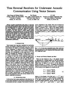
the slope of 6 qt (0) as a function of t. The results show that the slopes associated with all packets are approximately constant during the period of 50s. Note again that the residual phase jump can be further compensated by the PLL. 1

Temporal coherence

16 hydrophones was attached to free drifting Acoustic Oceanographic Buoy (AOB), with the first-top-hydrophone depth varying between 6.17-6.57 m. A carrier frequency fc = 12.5 kHz was used. A transmission packet is structured as follows: 50 LFM probe signals, each with 0.1s duration and 0.2s silence interval are first transmitted, then followed by a 100s BPSK signal which is pulse shaped with fourth root raise cosine pulse with roll-off factor of 0.5. Within the 100s data signal, an M-sequence of length 127 is embed at the beginning of each second. We consider six packets. The first four packets are transmitted sequentially with the source-array range increasing from 2.9 to 3.65 km and with the relative speed decreasing from 1.7 to 1.5 m/s based on the GPS data. Moreover, the last two packets are transmitted at around 10 minutes later with source-array range of 4.4-4.7 km and relative speed from 1.5 to 1.47 m/s. Here, in each packet we use the last LFM signal for IR estimation due to its close proximity to the data signal. Moreover, we consider only first 50s signal in each packet, where the Doppler frequency can be considered constant.

Pkt1 Pkt2 Pkt3 Pkt4 Pkt5 Pkt6

0.8 0.6 0.4 0.2 0 0

10

20

30

Time, t (sec.)

40

50

Figure 9: Temporal coherence of channel IRs with timewindowed probe IRs for RADAR07 data

Unwrapped ∠qt0 (0) (rad)

15

We also investigate the coherence of the time-windowed probe IRs and the IRs estimated from 50 M-sequences as shown in Figure 9. In this figure, the polynomial-fitted coherence curves, rather than the actual ones are shown for clarity of the presentation. We observe that the coherence time for all packets are shorter than 50s with the longest coherence time of 36s for packet 2.

(f )

10

5

Pkt1 Pkt2 Pkt3 Pkt4 Pkt5 Pkt6

0

−5 −400

−200

0

200

Figure 10 presents the temporal coherence based on the frequencyshifted probe IRs. We observe that the coherence times are improved for all packets and that of packet 2 is longer than 50s. Moreover, packets 5 and 6 have the coherence time of 45s increasing from 19s and 32s (shown in Figure 9), respectively. These results explain the superior performance of the FSpTR over the pTR and that of the FSpTR-DFE over the pTR-DFE as presented in Table 2. We observe that in packets 1 and 3, both the pTR and FSpTR perform poorly. This is due to the low coherence of the channel making the signals more prone to ISI and noise. However, since the DFE can mitigate the ISI problem, the performance of packets 1 and 3 improves significantly when the pTR-DFE and FSpTR-DFE are employed. The results in this section show that the benefit of using the FSpTR in the FSpTR-DFE is prominent for communications over rapidly time-varying channels. This is because the FSpTR can adapt to time-varying channels and ease the burden of the DFE to compensate for time-variations of the channels.

400

Frequency, f (Hz)

Slope of ∠qt (0) (rad/Hz)

0.04 Pkt1 Pkt2 Pkt3 Pkt4 Pkt5 Pkt6

0.035 0.03

(f )

0.025 0.02

0.015 0.01

0.005 0

10

20

30

Time, t (sec.)

40

50

(f )

Figure 8: Behaviors of qt (0) for the RADAR’07 data (f )

In this data set, the approximately linear functions of 6 qt0 (0) (based on the last LFM) with respect to f are also observed in all packets as shown in Figure 8 (upper). Moreover, using IRs (f ) estimated from the M-sequences, 6 qt (0) is calculated from the cross-correlation between these IRs and the time-windowed probe IRs estimated from the last LFM. Figure 8 (lower) presents

5

Conclusion

This work presents the FSpTR-DFE scheme, the combination of geometry-adapted pTR and adaptive DFE techniques for high data rate communications over time-varying shallow-water channels. The proposed scheme offers the performance enhancement to the FSpTR technique by using the adaptive DFE

ECUA 2010 Istanbul Conference

Vilaipornsawai, Silva, Jesus

Acknowledgements

Temporal coherence

1 Pkt1 Pkt2 Pkt3 Pkt4 Pkt5 Pkt6

0.8 0.6

This work is supported by European Commission’s Seventh Framework Programme through the grant for Underwater Acoustic Network (UAN) project (contract no. 225669). For the RADAR’07 data, the authors would like to thank FCT (Portugal) for funding the RADAR’07 sea trial under the RADAR project (POCTI/CTA/47719/2002). Our gratitude is also extended to all personnel involved in the experiment.

0.4 0.2 0 0

10

20

30

Time, t (sec.)

40

50

Figure 10: Temporal coherence of IRs with frequency shifted time-windowed probe IRs for RADAR’07 data

References [1] A. Silva. Environmental based Underwater Communications. PhD thesis, University of Algarve, 2009. [2] M. Stojanovic. Retrofocusing techniques for high rate acoustic communications. J. Acoust. Soc. Am., 117:1173– 1185, March 2005.

Table 2: MSE and BER performance of FSpTR and FSpTRDFE for RADAR’07 data Packet 1 2 3 4 5 6

fˆd -14.1 -14.27 -13.23 -12.67 -12.28 -11.99

Packet 1 2 3 4 5 6

pTR 3.4 -6.0 3.1 -4.3 -6.2 -5.9 pTR 49.6 0.73 46.2 2.6 2.1 0.79

FSpTR 3.2 -6.8 2.9 -4.9 -7.1 -6.6

MSE (dB) pTR-DFE -6.3 -10.8 -8.9 -9.7 -9.6 -12

FSpTR-DFE -8.2 -12.4 -10.3 -11.3 -13.8 -13.4

FSpTR 48.2 0.24 45.8 1.6 0.089 0.4

BER (%) pTR-DFE 2.6 0.32 0.67 0.72 0.92 0.017

FSpTR-DFE 0.37 0.003 0.07 0.056 0 0.0041

to further eliminate the residual ISI from the FSpTR. The MSE and BER performance of the FSpTR-DFE scheme is evaluated using the experimental data from RADAR’07 sea trial, and the simulated data of the south Elba island. In addition, the temporal coherence of the channels is investigated. Both data sets represent the scenario where the movement between the source and receiver is fast with relative speed of 1.5 m/s. The results show that the coherence has a strong impact on the performance of pTR-based techniques, and the FSpTR can increase the coherence. Moreover, the FSpTR-DFE outperforms the FSpTR and pTR-DFE considerably both in terms of MSE and BER. Furthermore, using the FSpTR-DFE, data transmissions with rate of 2000 BPSK sym/s with MSE of less than -8 dB can be realized in both data sets. These results encourage the use of the FSpTR-DFE scheme for high data rate, sustainable and reliable communications over rapidly time-varying underwater channels.

[3] G.F. Edelmann, H.C. Song, S. Kim, W.S. Hodgkiss, W.A. Kuperman and T. Akal. Underwater acoustic communications using time reversal. IEEE J. Ocean Eng., 30, no. 4:852–864, Oct. 2005. [4] T.C. Yang. Correlation-based decision-feedback equalizer for underwater acoustic communications. IEEE J. Ocean Eng., 30, no. 4:472–487, Oct. 2005. [5] H.C. Song, W.S. Hodgkiss, W.A. Kuperman, M. Stevenson and T. Akal. Improvement of time-reversal communications using adaptive channel equalizers. IEEE J. Ocean Eng., 31, no. 2:487–496, April 2006. [6] T.C. Yang. Temporal resolution of time-reversal and passive-phase conjugation for underwater acoustic communications. IEEE J. Ocean Eng., 28, no. 2:229–245, April 2003. [7] A. Silva J. Gomes and S. Jesus. Adaptive spatial combining for passive time-reversed communications. J. Acoust. Soc. Am., 124:1038–1053, Aug. 2008. [8] M. Stojanovic, J.A. Catipovic and J.G. Proakis. Phase coherent digital communications for underwater acoustic channels. IEEE J. Ocean Eng., 19, no. 1:100–111, Jan. 1994. [9] O.C. Rodriguez, A. Silva, F. Zabel and S.M. Jesus. The UAN interface: a web service for collaborative modeling. Proc. European Conference on Underwater Acoustics (ECUA’10), July 2010.