Combined Computational Approach Based on Density

Supporting Information:

Combined Computational Approach Based on Density Functional Theory and Artificial Neural Networks for Predicting The Solubility Parameters of Fullerenes J. Darío Perea,∗ ,† Stefan Langner,† Michael Salvador,†,‡ Janos Kontos,¶ Gabor Jarvas,¶ Florian Winkler,† Florian Machui,§ Andreas Görling,∥ Andras Dallos,¶ Tayebeh Ameri,† and Christoph J. Brabec∗ ,†,§ ∗

To whom correspondence should be addressed

†

Institute of Materials for Electronics and Energy Technology (i-MEET), FriedrichAlexander-Universität Erlangen-Nürnberg, Martensstrasse 7, 91058 Erlangen, Germany ‡

Instituto de Telecomunicações, Instituto Superior Tecnico, Av. Rovisco Pais, P-1049001 Lisboa, Portugal ¶

Department of Chemistry, University of Pannonia, H-8200 Veszprém, Egyetem street 10, Hungary §

Bavarian Center for Applied Energy Research (ZAE Bayern), Haberstrasse 2a, 91058 Erlangen, Germany ∥

Lehrstuhl für Theoretische Chemie and Interdisciplinary Center for Interface Controlled Processes, Friedrich-Alexander-Universität Erlangen-Nürnberg, Egerlandstrasse 3, 91058 Erlangen, Germany

Experimental Determination of Hansen Solubility Parameters The determination of absolute solubility was done by preparing oversaturated solutions of the fullerenes in binary solvent blends, followed by stirring for 24 hours at room temperature. Afterwards, the samples were centrifuged at 10000 rpm for five minutes. The centrifuged saturated solutions were subsequently diluted to allow measurements of the optical density. Absorption spectra were recorded using a Perkin Elmer Lambda-950 spectrometer from 300 S1

to 800 nm at room temperature. The absolute solubility for each solution was calculated by comparing its optical density to calibration curves with known concentration. The binary solvent gradient method (BGM) was employed to probe the surface of the Hansen sphere for a set of four different solvent mixtures. The solvent mixtures consist of a non-solvent and a "good" solvent. Each set consists of a fraction of chlorobenzene (CB) X / (X+Y) and a fraction of a non-solvent Y / (X+Y), where X+Y=100%. Chlorobenzene offers usually good solubility for many organic semiconductors used in organic electronic devices and is therefore used as processing solvent. As non-solvents we used: pyrimidine, 1-butanol, propylene carbonate, acetone, and cyclohexane. A series of solvent mixtures was prepared for each fullerene.

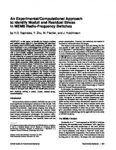
Solubility of Fullerenes For the determination of the Hansen Solubility Parameters (HSP) via the binary solvent gradient method (BGM) we defined a solubility limit of 10 mg/mL. The solubility spheres were calculated using the software HSP in Practice (HSPiP) [1], whereby values with higher concentration than the limit are inside the sphere. The solubility as a function of chlorobenzene (CB) content are depicted in Figures S1 – S4 for bis-[6,6]-phenyl-C61-butyric acid methyl ester (bisPC61BM), indene-C60 monoadduct (ICMA), indene-C60 bisadduct (ICBA) and [6,6]-phenyl-C71-butyric acid methyl ester (PC71BM). The dashed line in Figures S1 – S4 represent the solubility limit.

Figure S1 – Solubilities of bisPC61BM in chlorobenzene (CB) mixed with the non-solvents 1butanol, cyclohexane, propylene carbonate and acetone.

S2

Figure S2 – Solubilities of ICMA in chlorobenzene (CB) mixed with the non-solvents 1butanol, cyclohexane, propylene carbonate, acetone and pyrimidine.

Figure S3 – Solubilities of ICBA in chlorobenzene (CB) mixed with the non-solvents 1butanol, cyclohexane, propylene carbonate and acetone.

S3

Figure S4 – Solubilities of PC71BM in chlorobenzene (CB) mixed with the non-solvents cyclohexane, acetone, 2-propanol and dimethylsulfoxide.

COSMO Sigma-Moment Approach COSMO-RS provides an extended model based on -profiles physical components, named moments, to connect the molecular structure with thermodynamical properties. The moments of the screening charge density distribution (Fig. S5) represent linear descriptors derived from a regression function relating important material characteristics (P, sigma profile) to molecular properties [2]:

where MX i is the ith -moment. The coefficients (C0 –C15 ) can be derived by multilinear regression of the -moments with a sufficient number of reliable experimental data. Some of the 15 - moments have a well-defined physical meaning, e.g., surface area of the molecule: MX 0 = MX area , total charge: MX 1 = MX charge , electrostatic interaction energy: MX 2 = MX el, skewness of the -profile: MX 3 = MX skew, and acceptor and donor hydrogen bonding: MXHbacc3, MXHbdon3. However, the other moments (MX4, MX5, MX6, MXHbacc1,2,4, MXHbdon1,2,4) do not have simple physical interpretations [2] and have S4

merely mathematical rather than physical meaning. Therefore, they are solely included for quantitative structure property relationships (QSPR). COSMO Sigma-Profiles for Fullerenes

Figure S5- Visualization of the sigma profiles of the fullerenes under study as calculated using COSMO-RS.

Computational Procedure The 3D structures of the fullerenes considered in this study were built using HyperChemProfessional 7, which calculates the most stable conformational structures under the force field method. The raw 3D structures were exported as .pdb file format to Tmolex and were converted to Cartesian XYZ format. Molecular geometries were optimized by TURBOMOLE 6.3 quantum chemical program package using high quality quantum chemical ab-initio electronic structure optimization on the BP-TZVP-COSMO and BP-TZVP gas phase level. Sigma moments of molecules were calculated with COSMOtherm13 software using BP TZVP C21 1010 parameterization [3]. COSMO-RS sigma moments MX 1, MX 2, MX 3, MXHbacc3, and MXHbdon3 as quantitative structure property relationships (QSPRs) are used as the five input values for the Artificial Neural Network Toolbox of MATLAB (R2010b)[5]. The ANN learns to predict the output values of the properties of chemical S5

compounds on the basis of the input descriptor values. The most physical meaning interpretation sigma moments were employed.

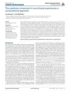
Figure S6- Visualization of the architecture of the optimized topology of the artificial neural network with 5 σ-moments using 5-12-1 Network [4]. Artificial Neuronal Networks (ANNs) Artificial neuronal networks (ANNs) are mathematical models based on the idea of neuronal cells brain functioning for information processing. They are used to estimate functions and results of systems that require large amounts of inputs. Generally, a set of selected inputs Xi (left hand side of the ANN in Figure S6) under study are associated with a function (right hand side of the ANN in Figure S6) via a group of weights Wi, which are chosen randomly in the first phase of the computational calculation - “training phase”. Afterwards, the software finds the correct weights using the trial and error technique, which involves iterative comparison of the resulting output with the desired output. During the ANN training phase, the training data is recorded together with the weights and functions inside the hidden layers (“synapse”). Then the values are inner validated and finally tested using an external database. To define the ANN’s topologies and to determine the numbers of neurons in the hidden layer, several ANN’s with different architectures were developed by simultaneous building of the ANN models and their validation. Models were constructed using the training set of compounds and a validation subset was used to provide an indication of the model performance using Levenberg–Marquardt back propagation training algorithms and mean squared error performance function. Since the models are nonlinear, the determination of the regression coefficients required iterative processes. To avoid “overtraining” phenomena, the ANN models obtained were firstly internally validated by the leave-many-out cross-validation technique and finally externally validated. 113 data points were chosen for training, 15 compounds were selected for post-training analysis (internal validation) and the test set were used for testing (external validation) [5].

S6

Figure S7- Schematic draw of ANN [1] S. Abbott, C.M. Hansen, H. Yamamoto, Hansen Solubility Parameters in Practice Complete with Software, Data and Examples, 4th ed.; 2013. ISBN: 9780955122026. Available from www.hansen-solubility.com. 
 [2] A. Klamt. COSMO-RS: From Quantum Chemistry to Fluid Phase Thermodynamics and Drug Design; Elsevier Science Ltd.; Amsterdam: 2005.
 [3] R. Ahlrichs, M. Bar, M. Haser, H. Horn, C. Kölmel, Electronic Structure Calculations on Workstation Computers: The Program System Turbomole. Chem. Phys. Lett. 1989, 162, 165-169. [4] F. Eckert, A. Klamt, COSMOtherm, Version C2.1, Release 01.10, COSMOlogic GmbH & Co. KG, Leverkusen, Germany, 2009.
 [5] Gabor Jarvas, Christian Quellet, and Andras Dallos, Estimation of Hansen Solubility Parameters Using Multivariate Nonlinear QSPR Modeling with COSMO Screening Charge Density Moments 
 Fluid Phase Equilibria. 2011, 309, 8-14.

S7