Combined Spatial and Temporal Effects of

Remote Sens. 2013, 5, 6513-6538; doi:10.3390/rs5126513 OPEN ACCESS

Remote Sensing ISSN 2072-4292 www.mdpi.com/journal/remotesensing Article

Combined Spatial and Temporal Effects of Environmental Controls on Long-Term Monthly NDVI in the Southern Africa Savanna Miguel A. Campo-Bescós 1,2, Rafael Muñoz-Carpena 1, Jane Southworth 3,*, Likai Zhu 3, Peter R. Waylen 3 and Erin Bunting 3 1

2

3

Agricultural and Biological Engineering Department, University of Florida, 287 Frazier Rogers Hall, P.O. Box 110570, Gainesville, FL 32611, USA; E-Mails: [email protected] (M.A.C.-B.); [email protected] (R.M.-C.) Projects and Rural Engineering Department, Public University of Navarre, Ed. Los Olivos, E-31006 Pamplona, Spain Geography Department, University of Florida, 3141 Turlington Hall, P.O. Box 117330, Gainesville, FL 32611, USA; E-Mails: [email protected] (L.Z.); [email protected] (P.R.W.); [email protected] (E.B.)

* Author to whom correspondence should be addressed; E-Mail: [email protected]; Tel.: +1-352-392-0494; Fax: +1-352-392-8855. Received: 15 September 2013; in revised form: 10 October 2013 / Accepted: 28 October 2013 / Published: 3 December 2013

Abstract: Deconstructing the drivers of large-scale vegetation change is critical to predicting and managing projected climate and land use changes that will affect regional vegetation cover in degraded or threated ecosystems. We investigate the shared dynamics of spatially variable vegetation across three large watersheds in the southern Africa savanna. Dynamic Factor Analysis (DFA), a multivariate time-series dimension reduction technique, was used to identify the most important physical drivers of regional vegetation change. We first evaluated the Advanced Very High Resolution Radiometer (AVHRR)- vs. the Moderate Resolution Imaging Spectroradiometer (MODIS)-based Normalized Difference Vegetation Index (NDVI) datasets across their overlapping period (2001–2010). NDVI follows a general pattern of cyclic seasonal variation, with distinct spatio-temporal patterns across physio-geographic regions. Both NDVI products produced similar DFA models, although MODIS was simulated better. Soil moisture and precipitation controlled NDVI for mean annual precipitation (MAP) < 750 mm, and above this, evaporation and mean temperature dominated. A second DFA with the full AVHRR (1982–2010) data found that for

Remote Sens. 2013, 5

6514

MAP < 750 mm, soil moisture and actual evapotranspiration control NDVI dynamics, followed by mean and maximum temperatures. Above 950 mm, actual evapotranspiration and precipitation dominate. The quantification of the combined spatio-temporal environmental drivers of NDVI expands our ability to understand landscape level changes in vegetation evaluated through remote sensing and improves the basis for the management of vulnerable regions, like the southern Africa savannas. Keywords: dynamic factor analysis; time-series analysis; NDVI; land cover change; climate change; temperature; mean annual precipitation; soil moisture; potential evapotranspiration

1. Introduction In southern Africa, long-term changes in the savanna ecosystem productivity and structure are believed to be driven by a combination of biotic (including human) and abiotic drivers [1–4], potentially representing irreversible landscape degradation [5]. Changes labeled “degradation” in the southern African savanna [6] are usually referring to the process of shrub encroachment (specifically, a shift from grass- and tree-dominated landscapes to less biologically productive landscapes dominated by scrub), and has been well documented throughout southern Africa [7–9]. Given this trend of potential degradation, understanding the temporal and spatial changes in vegetation dynamics and then identifying the dominant drivers responsible for these documented vegetation transitions is critically important for management, particularly in the context of increasing current climate variability and the increased future variability and climate change predicted for this region [10]. The critical importance of water is well recognized across savanna vegetation types (from open grassland savanna to densely wooded savanna) [11,12], although its role differs across vegetation types and biomes [13]. These studies have also demonstrated that fire regime, soils, herbivory, nutrients and land use also contribute to local patterns of ecosystem structure. However, a long-term simultaneous temporal and spatial analysis of the relative importance of the coupled relationship among environmental covariates driving savanna vegetation has not yet been performed at a monthly time-step using newly available 30+ year time series data. Thus, simultaneously identifying these spatial and temporal patterns of multiple, dynamic explanatory variables of importance, while accounting for unexplained, but shared, temporally varying trends on this longer time scale, is necessary to help improve our understanding of the controlling factors of vegetation response. The emergence and development of satellite remote sensing has provided an increasingly powerful instrument to monitor, observe and characterize landscapes, since it offers repeated data of large terrestrial areas at longer temporal scales, now from 1982 to 2010, which is a significantly long period of time to really begin to understand the drivers and changes to these biophysical systems [14–20]. Satellite-derived vegetation indices, such as the Enhanced Vegetation Index (EVI) and the Normalized Difference Vegetation Index (NDVI), have been linked with leaf area index, fraction of green vegetation and vegetation primary production [13,21]. Vegetation growth and biomass is impacted by multiple factors, including fire, herbivory, competition, soil properties and climate [22]. Among these factors, climate change effects on seasonal activity in terrestrial ecosystems are significant and well

Remote Sens. 2013, 5

6515

documented, especially in the middle and higher latitudes [23–26]. In arid and semiarid ecosystems and seasonally dry tropical climates where water is limited, vegetation growth is primarily constrained by water availability [14–17,27,28]. Rainfall stimulates green-up onset and determines the duration of growth and flowering of some desert plants, and its distribution in the rainy season is critical to vegetation germination, growth and biomass [29]. Tropical and sub-tropical regions of southern Africa are dominated by savannas, which are simply defined as the coexistence of trees and grasses. Savanna is considered a relatively productive ecosystem, with the entire African savanna biome accounting for 13.6% of the global net primary production (NPP) [30]. Understanding variations in the growing season that impact vegetation productivity is critical for the management of this particular ecosystem in which woody cover depends largely on mean annual precipitation (MAP) [2,3], but in which other factors, such as herbivory, fire and human activities (mainly grazing activities), can also exert a significant influence that is highly variable in space and time [3,31]. Time series approaches to continuous Earth observation-based variables are being adopted by many scholars to advance the understanding of inter- and intra-annual variations in vegetation and to examine and derive relationships between drivers of change and vegetation growth [2,3,32–40]. Application of wavelet analysis [41], Fourier analysis [42,43] and other transformations [44,45] all show promise in elucidating patterns of land cover variation, but rarely are multiple, spatiotemporally variable drivers of landscape change assessed simultaneously. To address this challenge, we will apply Dynamic Factor Analysis (DFA), a powerful multivariate times series dimension reduction technique, to investigate the dynamics of vegetation coverage across three large watersheds in southern Africa and two very different time scales, to identify the most important physical drivers of vegetation cover in the region. DFA was initially applied to economic time series [46–49] and was later extended to include explanatory variables in ecological systems. Because of its inherent advantages (efficiency, explanatory power, suitable for non-stationary data), it has since been applied successfully across a wide range of environmental systems, from the dynamics of squid populations [50] to variations in groundwater levels and quality [51–54], from soil moisture dynamics [55–57], to air quality [58] and, more recently, to link vegetation and climate dynamics [59–61]. In this study, we apply DFA to investigate the spatial and temporal interactions between NDVI and a collection of environmental covariates across the Kwando, Okavango and the upper Zambezi watersheds, which represent a dynamic savanna landscape in southern Africa. The specific objectives of this study were to (1) compare and validate a DFA NDVI model based on newly released Advanced Very High Resolution Radiometer (AVHRR) Global Inventory Monitoring and Modeling System third generation (GIMMS3g) data against an existing model based on the Moderate Resolution Imaging Spectroradiometer MODIS 10-year data and (2) develop a long-term model based on the 30+ years of AVHRR GIMMS3g NDVI data, to identify the driving factors that most fully explain the observed variation in the NDVI time series and how they vary across biophysical gradients. Part I of the paper will address a comparison between an adaptation of an existing decadal scale model, which utilizes MODIS NDVI data [61], and the newly available GIMMS3g NDVI dataset for their overlapping 2001–2010 time period. Part II will extend this validated (from Part I) AVHRR dataset to the full longterm period from 1982 to 2010 to determine the dominant physical drivers of vegetation growth across this four-nation southern Africa study region.

Remote Sens. 2013, 5

6516

2. Methods 2.1. Study Area The Okavango, Kwando and upper Zambezi catchments cover approximately 681,545 km2 in tropical and sub-tropical southern Africa (Zambia, Angola, Namibia and Botswana) (Figure 1). Mean annual precipitation (MAP) ranges from under 400 mm to 1,400 mm·yr 1 and is strongly correlated with latitude and elevation, with the highest rainfall in the mountainous north (Figure 1). Figure 1. Spatial pattern of mean annual Normalized Difference Vegetation Index (NDVI) (September–August of the next year) across the study area, derived from monthly NDVI Global Inventory Monitoring and Modeling System third generation (GIMMS3g) data from 1982 to 2010. The subset polygons correspond to mean annual precipitation intervals. The inset map shows the geographic location of the study area in southern Africa. MAP, mean annual precipitation.

This gradient straddles a previously noted [2] critical threshold of 650 mm, below which precipitation is believed to dominate savanna vegetation patterns and above which other factors, such as fire and herbivory, are hypothesized to play an important role. Relatively low human population in this region [62] reduces the effect of land use changes associated with major roads and settlements and facilitates identification of the explicit effects of climate on vegetation. The cattle stocking rate in this

Remote Sens. 2013, 5

6517

region is very low, with typical values lower than 10 head per km2 [63]. Within our study area, the southern semi-arid areas are characterized by low MAP and high interannual variability, and both the magnitude and relative reliability of MAP increases as we move towards the north [64]. Soils are primarily oxisols at higher elevations in the north and entisols in the south [65]. In particular, Kalahari sands characterize the majority of the area. Low topography in the south, especially in Caprivi (Namibia and northern Botswana), makes clear hydrologic separation of the catchments difficult. Inter-basin water historically flowed eastward, but these systems have not connected consistently since the late 1970s. 2.2. Remote Sensing and Climate Data 2.2.1. NDVI MODIS NDVI data (MOD13A3) were used in Part I of the analysis, along with the AVHRR GIMMS3g NDVI data product. MODIS provides monthly NDVI data at a 1-km spatial resolution in the sinusoidal projection. This product is generated using the 16-day 1-km MODIS VI output (created from between a maximum of 64 and a minimum of 1 observations, with 4 measures possible per day at the equator), temporally aggregated using a weighted average to create a calendar-month composite. Grids contaminated by clouds and those with average growing season NDVI less than 0.1 were excluded from analysis. The latest version of the Global Inventory Monitoring and Modeling System (GIMMS) NDVI dataset, termed NDVI3g (third generation GIMMS NDVI from AVHRR sensors), was used in both Part I and Part II of our study. It was generated from the AVHRR onboard a series of National Oceanic and Atmospheric Administration (NOAA) satellites (NOAA 7, 9, 11, 14, 16, 17 and 18) and with the goal of improving data quality in the northerly lands, where the growing seasons are short [1]. This dataset was previously developed by the Global Inventory Modeling and Mapping Studies (GIMMS) group, and was generated in the framework of the Global Inventory Monitoring and Modeling System (GIMMS) project at the National Aeronautics and Space Administration (NASA) Goddard Space Flight Center. No atmospheric correction is applied to the GIMMS data, except for volcanic stratospheric aerosol periods (1982–1984 and 1991–1994) [2]. A satellite orbital drift correction is performed using the empirical mode decomposition/reconstruction (EMD) method, minimizing the effects of orbital drift by removing common trends between time series of solar zenith angle (SZA) and NDVI [3]. Additionally, other deleterious issues, such as calibration loss and sensor degradation, were addressed [4]. The maximum NDVI value over a 15-day period is used to represent each 15-day interval, and this compositing scheme results in two maximum values of NDVI per month [1]. The entire available NDVI3g dataset spans from July 1981 to December 2011, with a spatial resolution of about 8 × 8 km. We aggregated the data into monthly observations using the maximum value composition, which further reduces cloud and other noise effects, and finally, we got the monthly NDVI for the entire study area from 1982 to 2010. 2.2.2. Climate Data In this study, we utilized the Matsuura and Willmott datasets of monthly precipitation (1982–2010) and monthly mean air temperature (1982–2010), which have a spatial resolution of 0.5 degrees by 0.5 degrees, with grid nodes centered on 0.25 degree (Table 1). These datasets improve upon a previous

Remote Sens. 2013, 5

6518

global mean monthly datasets with a refined Shepard interpolation algorithm and an increased number of neighboring station points included in the analysis [66]. Based on the grid nodes included in the three catchments, we interpolated the datasets into continuous surfaces with 1-km spatial resolution using inverse distance weighted interpolation. Global annual water budget data is available from the Willmott and Matsuura Global Climate Resource page [67]. The time series water budget data are available for seven variables: actual evapotranspiration, potential evapotranspiration, snowmelt, surplus, deficit, mid-monthly soil moisture and mid-monthly snow cover. This time series data is available at monthly time steps from 1900 to 2010; in this study, the actual evapotranspiration data was used for the timeframe of 1982 to 2010. Actual evapotranspiration (Ea) is the amount of water delivered to the atmosphere by evaporation and transpiration. It is determined by complex interactions of plant, soil and climatic variables, which, given the high spatial heterogeneity in savanna landscapes, makes such a measure influential. Potential evapotranspiration (E) impacts the water availability of vegetation and, therefore, can be an important factor influencing savanna ecosystems. The National Center for Environmental Prediction-Department of Energy (NCEP-DOE) Reanalysis II global potential evaporative rate data from 1982 to 2010 were used to represent the environmental demand for evapotranspiration (Table 1, [67–69]). NCEP-DOE Reanalysis II provides monthly data at about a 2.5-degree spatial resolution in the Network Common Data Form (NetCDF) format. Since the Gaussian grids are irregular, we converted NetCDF to feature layers by month using the “Make NetCDF Feature Layer” tool in ArcGIS software (ESRI, Readlands, CA, USA) and interpolated to continuous surfaces with a 1-km spatial resolution using an inverse distance interpolation method. Table 1. Initial set of candidate explanatory variables and their sources. CPC, Climate Prediction Center. NCEP-DOE, National Center for Environmental Prediction-Department of Energy. Symbol

Source

Matsuura and Willmott’s Monthly Precipitation

Dataset

P

[67]

Matsuura and Willmott’s Monthly Mean Temperature NCEP-DOE Reanalysis II Monthly Minimum Temperature NCEP-DOE Reanalysis II Monthly Maximum Temperature CPC Monthly Soil Moisture Matsuura and Willmott’s Monthly Actual Evapotranspiration

T m M S Ea

[67] [68] [68] [68] [67]

NCEP-DOE Reanalysis II Monthly Potential Evapotranspiration NCEP-DOE Reanalysis II Monthly Vapor Pressure Deficit Monthly Southern Oscillation Index

E V O

[68] [68] [69]

Soil moisture (S) is an integrated factor that exerts dominant control on the spatial distribution of trees, shrubs and grasses. The Climate Prediction Center (CPC) global monthly soil moisture data from 1982 to 2010 were used, which provides monthly values at a 0.5-degree spatial resolution with grid nodes centered on 0.25 degrees (Table 1). This dataset is based on the land model, a one-layer “bucket” water balance model, which uses CPC monthly global precipitation data over land and monthly global temperature for global reanalysis as the input fields [70]. We interpolated the datasets into continuous surfaces with a 1-km spatial resolution using inverse distance weighted interpolation.

Remote Sens. 2013, 5

6519

Vapor pressure deficit (V), defined as the difference between the saturation and actual vapor pressure, is an accurate indicator of the actual evaporative capacity of the air. It is an integrative climate variable, which can impact water-sensitive savanna systems. We calculated the monthly V data from 1982 to 2010 from NCEP-DOE Reanalysis II monthly maximum temperature, monthly minimum temperature and monthly mean relative humidity. The calculation procedures for monthly V are shown as follows. The saturation vapor pressure can be calculated from air temperature, which is expressed by: eo (T ) = 0.6108exp[

17.27T ] T + 237.3

(1)

where e0(T) is saturation vapor pressure at the air temperature, T (kPa), T is air temperature (°C) and exp is natural logarithm. Due to the non-linearity of the above equation, the mean saturation vapor pressure of a month should be calculated as the mean between the saturation vapor pressure at the mean maximum and minimum air temperatures for that month:

eo (Tmax ) + eo (Tmin ) 2 where es is the mean saturation vapor pressure. The actual vapor pressure can be calculated as: es =

(2)

RH mean (3) 100 where RHmean is the mean relative humidity and ea is the mean actual vapor pressure. The mean V of a month can be computed as: V = es − ea (1) ea = es ×

Likewise, the derived V gridded layers at a 1-km spatial resolution were used to extract monthly mean V values of each polygon defined by different precipitation intervals. The Monthly Southern Oscillation Index (O) data was obtained from the Australian Government Bureau of Meteorology [69]. This index gives an indication of the development and intensity of El Nino Southern Oscillation (ENSO) events in the Pacific Ocean at a monthly time-step. The difference in pressure between Tahiti and Darwin is used to calculate O, where significant negative values (< 8) indicate El Niño events and positive values (>8) indicate La Niña events. Such measures are important to models of savanna land cover, as ENSO events can impact the precipitation and wind patterns across southern Africa. 2.3. Conceptual Basis for Analysis Monthly NDVI data are used as the indicator of vegetation dynamics and change and as the response (dependent) variable in the analysis. A suite of climate variables (Table 1) were used as candidate explanatory (independent) variables (CEVs) in the analysis: precipitation (P), mean temperature (T), minimum temperature (m), maximum temperature (M), soil moisture (S), vapor pressure deficit (V), actual evapotranspiration (Ea), potential evapotranspiration (E) and the Southern Oscillation Index (O). These variables were selected, due to their presence in the literature as potential drivers of NDVI or vegetation growth and also for being readily available at the necessary spatial and temporal resolutions for this study. Due to many climate data being used in the calculations of other variables (e.g., temperature and precipitation in evapotranspiration measures, etc.), additional analyses

Remote Sens. 2013, 5

6520

had to be undertaken to remove some potentially overlapping variables, and this also inherently restricted the datasets available for use. Herbivory and fire are additional variables that the literature discusses as having potential impacts in savanna landscapes [2,3,31]. Although monthly time series data of herbivory were not available for the study region, the very low cattle stocking rate (250 head/km2 in other African savanna regions) [63] and low density of wildlife management areas suggest that herbivory effect is likely minimal at the more extensive polygon level used in this analysis. Savannas are the most frequently burnt ecosystems, and fire is regarded as the dominant process preventing savanna trees from achieving their resource-driven potential [3,11]. Since the AVHRR GIMMS project does not contain long-term monthly fire data and it cannot be obtained elsewhere at an appropriate scale, these will not be model inputs, but rather, will be represented by the unexplained variance in the DFA model (common trends) as explained below. Time series of explanatory and response variables were then aggregated up from a pixel-scale by extracting the mean values over specific polygon regions as defined by 50-mm precipitation intervals. This was done across the landscape subdivided for each of the drainage basins and resulted in the production of 48 individual data polygons (Figure 1). While the dominant precipitation gradient across the study area is from the north (higher elevation) to the south (lower elevation), there are also drivers (topography, oceanic influence, etc.) from east to west. As such, the use of three drainage basins may help to pick up differences in these drivers across the east-west gradient. Ultimately, 48 individual polygons were created based on MAP polygons and drainage basin locations shown in Figure 1, yielding an initial set of 433 time series: 1 response variable, 8 CEVs in each of the 48 polygons and one CEV for the whole domain (O). 2.4. Dynamic Factor Analysis (DFA) DFA is a statistical methodology designed to explore common patterns evident in the relationships and interactions between response and explanatory time series. Therefore, a priori knowledge of the dynamics amid response (NDVI) and explanatory (e.g., precipitation, fire, etc.) variables is not needed to successfully apply this tool [53]. Unlike other time series methods, DFA is capable of modeling relatively short, incomplete, non-stationary time series [71]. Intrinsically a structural time series technique [48], DFA provides the means to model temporal variation in observed data (response variables) as linear combinations of common trends, explanatory variables, a constant intercept and noise [48,49,71]. Together, these parameters represent the unexplained variability (common trends) and explained variability (explanatory variables) to create the following model: (2) (3) where Sn(t) is a vector comprised of the set of N response variables (n = 1,…,N), c(t) is a vector comprised of the C common trends (c = 1,…,C), c,n are factor loadings (weighting coefficients) indicative of the weight associated with each of the common trends within the Dynamic Factor Model (DFM), n is a constant level parameter, k(t) is a vector comprised of the K explanatory variables (k = 0,…,K) and k,n are regression coefficients representing the relative importance of each

Remote Sens. 2013, 5

6521

explanatory variable. In this study, Sn signifies the 48 NDVI time series (one from each polygon in Figure 1). n(t) and m(t) are independent Gaussian noise terms with zero mean and an unknown diagonal or symmetric/non-diagonal covariance matrix. Common trends are obtained using the Kalman filter/smoothing algorithm and the expectation maximization (EM) technique [72–74] and are modeled as a random walk [48]. The EM technique is also used to calculate level parameters ( n) and factor loadings ( c,n), which denote the relative importance of the common trends. Regression coefficients ( k,n), which indicate the relative spatial importance of explanatory variables, are modeled using multi-linear regression [50]. Canonical correlation coefficients ( c,n) were employed to quantify the cross-correlation evident between response variables and common trends, with values of c,n close to unity, indicating high correlation. The significance of the relationship between response and explanatory variables was based on the magnitude of the k,n and the associated standard errors (significant for t-values > 2). To produce models with a minimum number of common trends, the use of non-diagonal error covariance matrices was employed [75]. As with other modeling tools, DFA aims to balance model parsimony while maintaining the goodness-of-fit. By developing different dynamic factor models (DFM), this balance can be evaluated. The performance of each developed DFM was evaluated using the Nash and Sutcliffe [76] coefficient of efficiency (Ceff) with a statistical significance test [77] and the Bayesian information criterion (BIC) [78]. Ceff compares the variance between predicted and observed data about the 1:1 line, with Ceff = 1 indicating that the plot of predicted vs. observed data matches the 1:1 line [76]. The BIC is a statistical measure for model selection that rewards goodness-of-fit, but penalizes increases in the number of model parameters. The DFM that minimizes the number of common trends required to achieve the best fit, as determined by the Ceff and/or BIC, is considered to be the best model. The addition of appropriate explanatory variables may help to improve the performance of the model, identify environmental factors (if any) that affect the response variables and quantify the spatial distribution of the weight of each factor. To directly compare the relative importance of common trends and explanatory variables across a response variable domain, all response and explanatory variables were normalized (mean subtracted, divided by standard deviation) prior to analysis [50,79]. DFA was implemented using the Brodgar Version 2.7.2 statistical package (Highland Statistics Ltd., Newburgh, UK), which uses the statistical software, R, Version 2.9.1 (R Core Development Team, Viena, Austria, 2009). 2.4.1. Dimension Reduction of Candidate Explanatory Variables Nine available candidate explanatory variables (CEV) were initially considered (Table 1). Based on Campo-Bescós et al. [61], we used the regional weighted-average of 8 CEVs, excluding O, since it was found to capture the major variance of each CEV across all polygons. The variance inflation factor (VIF) was used to quantify the severity of the collinearity of each set of CEVs [75]. The authors recommend using a backward selection method to remove one variable at a time (the one with the highest VIF > 10) and recalculate VIF after each iteration, until we obtain a set of non-collinear variables. Thus, in an initial reduction step, CEVs with VIF > 10 were excluded from the analysis [75,80,81].

Remote Sens. 2013, 5

6522

2.4.2. NDVI Analysis Procedure The DFA analysis followed a three stage process. (1) Model I: DFMs were developed based on increasing numbers of common trends (without CEVs) to establish a baseline satisfactory model performance according to goodness-of-fit indicators. (2) Model II: different combinations of CEVs were incorporated to reduce unexplained variability and improve the goodness-of-fit. (3) Model III: the common trends (unexplained variation) were removed, while optimizing multi-linear models of the best CEVs identified in Model II. Multiple regression code in Matlab (v2013a, The MathWorks, Inc., Natick, MA, USA) was used in the optimization process. Model III permitted refining of the selection of the most important CEVs, since inclusion of trends in Model II may mask the effects of important explanatory variables of the multivariate model (2). When selecting the “best” model, we adopted a multi-criteria objective consisting of: (a) model adequacy (minimizing BIC); (b) global model goodness-of-fit (maximizing average Ceff); (c) improvement in Ceff for the worst-performing polygons (minimizing range in Ceff); and (d) reduction in the importance of common trends (i.e., minimizing c,n). 3. Results 3.1. Part I: Comparison of MODIS and AVHRR Models (2001–2010) Figure 2 shows the overlap time period for both weighted-area average NDVI estimations, AVHRR and MODIS. The time period of overlap is from 2001 to 2010, and the associated correlation coefficient is 0.95. While the correlation and trends (Figure 2) are similar, they exhibit differences during the peaks resulting from differences in sensors, time points within the month (from which maximum NDVI is obtained) and the frequency of measures (MODIS being more frequent, with often daily observations being integrated into the monthly measures). As such, differences in the values measured are to be expected, and although their correlations and overall trends do match well, MODIS provides improved spatial, spectral and radiometric resolutions compared to the AVHRR measures. Figure 2. Variability of observed average Normalized Difference Vegetation Index (NDVI) estimated from the Moderate Resolution Imaging Spectroradiometer (MODIS) (black line) and the Advanced Very High Resolution Radiometer (AVHRR) (red line) from 2001 to 2010.

Remote Sens. 2013, 5

6523

The DFA model performance for MODIS NDVI and AVHRR NDVI3g was compared for the same suite of CEV and the same model type (multi-linear regression used in a previous study [61]: precipitation (P), mean temperature (T), maximum temperature (M), fire (F), soil moisture (S) and potential evapotranspiration (E). Due to the good performance of Model III (multi-linear regression, after removal of common trends) in the previous study, we compared the consistency of this model type for both datasets. For only one CEV (Figure 3), good consistency is found for all the individual CEVs, where F is the variable that itself explains a higher percentage of NDVI variance, followed by E. However, because the NDVI time series is not identical from both sources, goodness of fit differs. In general terms, MODIS NDVI is better predicted than the AVHRR NDVI3g (Ceff). Incremental improvement of the multi-linear regression model performance with the addition of explanatory variables (Table 2) follows the same pattern for both datasets. The best model includes five CEVs that match those selected in the previous study [61]: F, S, P, T and E (Table 2). Figure 3. Dynamic Factor Analysis (DFA) model performance with one explanatory variable. The response variable, NDVI, is from MODIS (black circles) and from AVHRR (red triangles). The range of Ceff is presented across polygons. (Ceff, Nash-Sutcliffe efficient coefficient; BIC, Bayesian information criterion). 0.90 0.80 0.70 0.60 0.50 0.40 0.30 0.20 0.10 0.00

–7,000 –6,000 –5,000 –4,000 –3,000 –2,000 –1,000 , , , , , , ,

0

1,000 ,

Table 2. Incremental best model, with the addition of the addition of the explanatory variables. Ceff presented are calculated for the whole area (values in parenthesis represent range for polygons). (Ceff: Nash-Sutcliffe Efficient Coefficient). NDVI MODIS

AVHRR

F FS FSP

0.70 (0.51–0.81) 0.82 (0.70–0.87) 0.89 (0.81–0.92)

0.67 (0.42–0.79) 0.80 (0.55–0.88) 0.81 (0.59–0.90)

FSPT FSPTE

0.90 (0.86–0.92) 0.91 (0.88–0.93)

0.82 (0.66–0.90) 0.83 (0.66–0.91)

F, fire; S, soil moisture; P, precipitation; T, mean temperature; E, potential evapotranspiration.

Remote Sens. 2013, 5

6524

Figure 4. The weight of each driver for the best NDVI model and goodness of fit along the mean annual precipitation (MAP) and ecological gradients. The upper panel shows the variation in the Nash and Sutcliffe coefficient of efficiency (Ceff) for MODIS (in black) and AVHRR (in red). The bars show the mean and range of values across watersheds. The lower panel shows the main trajectories in the weighting coefficients for candidate explanatory variables (CEVs) for predicted NDVI values across the MAP gradient (MODIS in black; AVHRR in red). The weighting coefficients for CEVs are shown by symbols corresponding to the labels. Trend lines represent the main trajectories and highlight the shift in the importance of environmental drivers for each NDVI predicted.

For the extended time period analyzed in this study, 1982 to 2010 (Part II), the F time series is not available. Therefore, the best model without F included four CEVs: S, P, T and E (Table 2). Again, MODIS NDVI is better predicted than AVHRR, with a Ceff value of 0.86 (0.77–0.91) and 0.72 (0.40–0.88), respectively. The spatial importance of each CEV follows similar patterns in both models (Figure 4). In the drier area (MAP < 750 mm) dominated by grassy vegetation, S is the key factor independent of the NDVI source. In these subregions, ranking of weighting coefficients are equal for both NDVI signals. For wet MAP regions > 950 mm, dominated by woody vegetation, the NDVI signal is also modeled across the domain with similar factor importance, and as described in the previous study [61], E is the main driver and negatively related with NDVI. In this subregion, T and P exhibit also a stronger weight on NDVI from MODIS than from AVHRR. The goodness-of-fit of NDVI (top panel in Figure 4) from AVHRR reaches the lowest values in the humid region. In the previous study, F was highlighted as one of the main drivers of MODIS NDVI in this humid region [61]. Considering the coarser temporal resolution of the raw AVHRR time series, the impact of F can be higher on AVHRR than on MODIS time series, with a higher raw temporal resolution. While monthly MODIS NDVI is based on numerous

Remote Sens. 2013, 5

6525

measurements per month, AVHRR has only two measurements per month. Clouds can affect AVHRR NDVI the same way as fire, especially in the humid area. Therefore, this explains the lower predictions for this humid area in which results need to be interpreted carefully. In all, the consistent models obtained for both datasets indicate that, in spite of the dataset differences, for the overlapping period, both datasets include similar dynamics that are explained by the same environmental drivers. 3.2. PART II: Long-Term AVHRR Models (1982–2010) 3.2.1. Experimental Time Series Monthly NDVI data collected between 1982 and 2010 showed relatively consistent seasonal cycling, typical for this region, across all data analysis precipitation polygons (Figure 5). Figure 5. Variability of observed NDVI for the study region for two mean annual precipitation (MAP) ranges. Upper and lower extremes values and range for MAP > 750 mm (continuous lines and light shading) and MAP < 750 mm (broken lines and dark shading).

Differences of patterns (maximum values) are observed between humid and drier regions. Humid areas (MAP > 950 mm) exhibited some NDVI reductions at the maximum photosynthetic period. This fact can be related to punctual anomalies, such as clouds and fires; for example, for clouds, a period of maximum NDVI is correlated to high precipitation and, therefore, to a high frequency of clouds. 3.2.2. Selection of Candidate Explanatory Variables Following the procedure described in the previous section, we used the set of variables that do not suffer from collinearity across variables (variance inflation factor, VIF < 10, [75]). Variables with VIF > 10 were removed and the VIF recalculated after each iteration (Step 1–2 in Table 3), until we obtained a set of non-collinear variables. The final set of CEVs resulted in the selection of eight CEVs

Remote Sens. 2013, 5

6526

for further investigation, consisting of monthly time series for 1982–2010 of precipitation (P), mean temperature (T), minimum temperature (m), maximum temperature (M), soil moisture (S), actual evapotranspiration (Ea), potential evapotranspiration (E) and the Southern Oscillation Index (O) (Table 1, Figure 6). We used weighted-average variables as explanatory variables. Figure 6. Normalized, area-weighted average explanatory variables used in the study. (A) Precipitation, P; (B) mean temperature, T; (C) minimum temperature, m; (D) maximum temperature, M; (E) soil moisture, S; (F) actual evapotranspiration, Ea; (G) potential evapotranspiration, E; (H) Southern Oscillation Index, O; and (I) common trend (C) of Model II.

Remote Sens. 2013, 5

6527

Table 3. Test of collinearity of explanatory variables. The final set of explanatory variables selected based on variance inflation factor (VIF) < 10 are shown in bold. VIF values were calculated for area-weighted time series for the region. Variable Symbol

VIF Step 1

Step 2

P

4.9

4.4

T m M S

9.8 9.8 12.1 2.2

8.4 8.6 5.5 2.1

Ea E V O

11.5 7.5 33.9 1.0

7.2 5.5 1.0

Explanatory variables are: precipitation (P), mean temperature (T), minimum temperature (m), maximum temperature (M), soil moisture (S), actual evapotranspiration (Ea), potential evapotranspiration (E), vapor pressure deficit (V) and Southern Oscillation Index (O).

3.2.3. DFA Models (I, II and III) The first model was developed as a baseline using only an increasing number of common trends (Model I; Table 4) and no explanatory variables. The best, Model I, was obtained with one common trend (C = 1), sufficient to minimize the BIC indicator and achieving the highest overall Ceff of 0.79 (ranging between 0.34 and 0.95 across precipitation polygons) (Table 4). The single common trend illustrated shared variability across the 48 NDVI time series and may be viewed as a general signature of NDVI across the domain, integrating environmental factors that influence vegetation dynamics. 0.97) between the 48 NDVI response variables and However, high positive correlation (0.59 c,n the common trend highlights that the model captures the principal variability of NDVI across the domain. Nevertheless, since this trend explains a latent effect (unexplained variance), it does not reveal which biophysical variables are driving NDVI variations. Next, in order to reduce model reliance on the unexplained variability in Model I, we developed DFA with explanatory variables and common trends (Model II, Table 4). Combinations of weighted-area average CEV time series were evaluated in a factorial manner to determine the best model fits (255 DFMs were explored between one and four common trends; see details in the Supplementary Material). The best model in order of BIC criteria was Ea, T and S (C = 1 and K = 3, BIC = 8,538; bold text in Table 4), which has one explanatory variable (Figure 6I) and three explanatory variables: actual evapotranspiration (Ea, Figure 6F), mean temperature (T, Figure 6B) and soil moisture (S, Figure 6E). Based on statistical significance (p = 0.01), the model had an acceptable model performance with an overall Ceff = 0.77 [77]. In comparison with Model I, Model II improves model performance for the worst performing polygons, from 0.34 to 0.46. Finally, the explanation of response variables was shifted from unknown (common trend) to known drivers (explanatory variables), with a decrease of average canonical correlation from 0.89 to 0.06 (Model I and II, respectively). Figure 7 shows the weight of each driver for Model II Ea, T and S and the

Remote Sens. 2013, 5

6528

goodness-of-fit along each MAP gradient across the study area. Over the range of MAP, the importance of the common trend is not statistically significant (t-test < 2), illustrating a latent effect equally distributed across the domain. According to Figure 7, S and Ea are the main drivers of NDVI in the savanna grassland (MAP < 750 mm). However, the rate of change on S and Ea over the savanna grassland is opposite. Thus, Ea rises in importance with MAP, while S decreases. T is the third driving factor of NDVI of importance in this region, with a homogeneous influence across the domain (Figure 7). Over a MAP > 950, Ea overcomes this key factor. Its importance is homogeneous across the humid range. The second driving factor in the more wooded savanna is T. As well as Ea, T exhibits a constant pattern across this region. However, its importance is half or lower than Ea. Table 4. Selected results of the dynamic factor analysis of NDVI for the long-term AVHRR-based models (1982–2010). Numbers in bold represent selected models. Model a

No. of Trends (C)

Explanatory Variables

No. of Parameters

BIC b

Ceff c

p-value d

1 2 3

-

1,272 1,319 1,365

8,186 8,083 7,909

0.79 (0.34–0.95) 0.79 (0.34–0.95) 0.80 (0.37–0.95)

+ + +

0.89 (0.59–0.97)

I

1 1 1 1

Ea Ea M Ea T S Ea T S P

1,320 1,368 1,416 1,464

8,256 8,531 8,538 8,293

0.78 (0.36–0.90) 0.74 (0.37–0.87) 0.77 (0.46–0.87) 0.79 (0.52–0.87)

+ + + +

1

Ea T S P M

1,512

8,027

0.81 (0.53–0.89)

+

0.57 (0.33–0.68) 0.06 ( 0.01–0.11) 0.06 ( 0.01–0.11) 0.06 ( 0.02–0.11) 0.06 ( 0.02–0.11)

0 0

Ea Ea M

96 144

13,766 20,980

0.58 (0.23–0.76) 0.74 (0.36–0.86)

+

0 0 0

Ea M P Ea T S P Ea T S P M

192 240 288

22,830 23,506 24,333

0.77 (0.44–0.87) 0.79 (0.52–0.87) 0.80 (0.53–0.88)

+ + +

II

III

a

1,n

e

Model I: only common trends (unexplained variability); Model II: with common trends and explanatory variables

(explained variability); Model III: only explanatory variables (from multiple regression). criterion.

c

b

BIC: Bayesian information

Ceff: Nash-Sutcliffe coefficient of efficiency. Values presented are calculated for the whole area (values in

parenthesis represent the range for polygons).

d

Classification of goodness-of-fitness results based on statistical

significance (p = 0.01) for the whole region: , Unsatisfactory; +, acceptable; ++, good [77]. e

1,n:

Canonical correlation

coefficients for the first common trend of Models I and II.

The multi-linear regression model selection (Model III) is presented in Figure 8, showing incremental improvement of Model III performance with the addition of the explanatory variables. Minimum BIC is achieved with five explanatory variables (BIC = 24,333). Thus, the best model fit is model Ea, T, S, P and M with a Ceff of 0.80 (Model III, bold text in Table 4), which relates to the explanatory variables of evapotranspiration, mean temperature, soil moisture, precipitation and maximum temperature.

Remote Sens. 2013, 5 Figure 7. The weight of each driver for the best NDVI model and goodness-of-fit along the mean annual precipitation (MAP) gradients for Model II. Lines represent the main trajectories and highlight the shift in the importance of environmental drivers for each NDVI zone predicted (see details in the caption of Figure 4). Symbols are filled in red where the weighting coefficients are significant (t-value > 2).

Figure 8. The incremental improvement of Model III performance with the addition of the explanatory variables. The best model is shown in bold; the solid line shows weighted averages and dashed lines the range across the spatial domain.

6529

Remote Sens. 2013, 5

6530

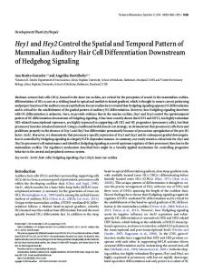
Figure 9 shows the weight of each driver for this best model and the goodness-of-fit along each MAP gradient. This analysis found that soil moisture was the most important variable, followed by actual evapotranspiration, with a more minor impact of temperature when the MAP was below 950 mm. Above 950 mm, soil moisture and mean temperature become insignificant, and actual evapotranspiration and precipitation dominate as drivers of NDVI. Notice that the flat response of maximum temperature (M) does not mean it is not important (or needed). M is adding temporal structure to the model (explains temporal variance), but does so equally across the domain (spatially). Figure 9. The weight of each driver for the best NDVI model and the goodness-of-fit along the mean annual precipitation (MAP) gradient for Model III. Lines represent the main trajectories and highlight the shift in the importance of environmental drivers for each NDVI zone predicted (see details in the caption of Figure 4). Symbols are filled in red where the weighting coefficients are significant (t-value > 2). In the image, separate use en dash for ranges, thousands with a comma, and are Ea, M, P, S, T, E, etc., italicized?

4. Discussion Zhu and Southworth [13] found a significant positive relationship between mean annual NPP and MAP for the bush/scrub and grassland savanna regions, but no relationship in wooded savannas. Specifically, they found a relationship with NPP and MAP up until around 850–900 mm, above which no relationship existed. In this study, many more variables have been included in determining the controlling factors on NDVI across this landscape. Across a thirty-year time series, which is long enough to detect significant changes and patterns in vegetation cover, the key drivers were soil moisture, followed by actual evapotranspiration, with a more minor impact of mean temperature when MAP was below 950 mm. Above 950 mm, soil moisture and mean temperature become insignificant and actual evapotranspiration and precipitation dominate as drivers of NDVI. This switch, as with the

Remote Sens. 2013, 5

6531

Zhu and Southworth [13] study of NPP patterns, occurs around the transition from shrub/scrub and grassland savannas to more wooded savanna environments. It is important to highlight that for the overlap time period between MODIS and AVHRR (2001–2010), the two variables, Ea and F, have a high correlation coefficient (r = 0.84). In fact, Ea has the highest correlation variable with F, followed by P (r = 0.63). As such, the variable, Ea, seems to encompass some of the unavailable fire variable in this Part II model development and also causes differing patterns and trends with the remaining variables, due to its inclusion. However, at the time scale of 1981–2011, these variables were not correlated to such a degree and, hence, could be included in this model together (in the Part I model, Ea was removed, due to collinearity with other variables). The models developed in Part I and Part II of this paper are therefore not possible to compare fully, as different variables were used in their creation, in accordance with the rules of the model development and variable selection. Additionally, the model developed in Part II did not include fire, as this variable in Part I was derived from the MODIS data itself, which does not extend back pre-2000. The results of the long-term analysis with AVHRR NDVI highlight the shift in importance of driving forces over the region in areas that receive different amounts of mean annual precipitation (MAP) representing three distinct savanna types (from grass to tree dominated systems). For example, for the subregion, where MAP < 750 mm (primarily grass-dominated savannas), our analysis shows that NDVI was most strongly influenced by soil moisture, maximum temperature and actual evapotranspiration, whose impact increases with increasing precipitation, with much smaller effects of precipitation. The importance of soil moisture found for grass-dominated savannas strongly supports the broader view of savannas proposed by Ward et al. [82] and the need to incorporate soil-climate interactions and not focus so strongly on fire-climate restrictions. In these very low moisture environments, the intermediary of the soil and its ability to hold and store moisture (rather than just the precipitation amount per se) is key. Linhoss et al. [83] also identified soil moisture as a key driver of the environmental dynamics in the Okavango Delta. On the other hand, regions with MAP > ~950 mm (where NDVI and overall biomass tend to increase with an increasing presence of woody vegetation) presents markedly different patterns. In these more humid areas (up to 1,300 mm MAP), actual evapotranspiration dominates, followed in importance by precipitation and mean temperatures, while the importance of soil moisture declines (as vegetation is no longer as water limited). Previous studies suggest that for arid and semi-arid areas, increasing pre-season temperature could reduce water availability by increasing evaporation, thereby delaying the season onset [16]. However, if we view the key variables across the region as a group, we actually see that moisture and moisture availability do dominate the controls in this water-limited environment. Specifically, soil moisture dominates below 950 mm, a measure of the actual moisture content (precipitation and soil type/topography combined), and above 950 mm, actual evapotranspiration (available water) and precipitation are dominant. All three of these variables link to water availability as the strongest control on plant growth. As such, this does corroborate the findings of previous researchers, that in arid and semiarid ecosystems and seasonally dry tropical climates where water is limited, vegetation growth is primarily constrained by water availability [14–17,27,28]. This relates to the mechanisms where precipitation stimulates green-up onset, and its distribution in the rainy season is critical to vegetation germination, growth and biomass [29]. The results of this study reveal the power of DFA to aid in the interpretation of spatially variable environmental effects on a parameter of interest. In

Remote Sens. 2013, 5

6532

particular, this analysis quantified the spatial pattern of the role of each environmental factor in determining the resultant NDVI across an extensive, heterogeneous domain, specifically highlighting the transition between regions of bush/grass vs. tree savanna, a key class of interest within savanna research. The removal of common trends from the final DFM in Model III yields a statistical model of NDVI based solely on a set of biophysical parameters. It is therefore possible to make predictions about changing NDVI in the study region based on the relevant environmental drivers and how they may change due to mid- and long-term climate forcing. While application of Model III for this purpose may provide a “first-cut” approximation of the likely response of vegetation to changing climate (via NDVI), it is important to recognize that the models developed herein are statistical; as such, any forecasting model inherently assumes that the multivariate relationships identified in the DFA remain consistent across a different collection of climatic variables (a problematic assumption under non-stationary climate conditions). While the sign of the identified relationships may not change over different boundary conditions, the slope and magnitude almost certainly will. The lengths of some remote sensing records, such as the newly released AVHRR GIMMS NDVI3g, now permit a more systematic quantification of key relationships between the drivers of vegetation growth and the resulting cover type over a sufficiently extensive spatial and temporal scale to allow us to start to develop models for potential use under future climate change scenarios. In addition, we can reverse the model predictions and use them to determine where the model underperformed and, thus, what type of changes may be occurring in the landscape locations and what their drivers may be that were not included in the larger model. This type of change detection analysis will be used in future research across this landscape. This approach will help in improving the understanding of savanna dynamics for vegetation growth, in identifying potentially missed drivers and also in assessing the likely impacts of future climate variability and change in this very sensitive region of the world. 5. Conclusions Dynamic factor analysis was applied to study the variation in NDVI across three co-located extensive watersheds in southern Africa and, more specifically, to identify the driving factors explaining the observed variation in savanna vegetation cover time series and their variation across biophysical gradients. Through the use of such models as NDVI, we can improve our understanding of these savanna systems, better evaluate their drivers and, so, hopefully utilize these studies in future change studies and for management purposes. This improvement in our ability to characterize these savanna landscapes allows for a much more solid footing upon which examinations of the change mechanisms and drivers are based. We first evaluated AVHRR- vs. MODIS-based NDVI datasets across their overlapping period (2001–2010). NDVI follows a general pattern of cyclic seasonal variation, with distinct spatio-temporal patterns across physio-geographic regions. Both NDVI products produced similar DFA models, although MODIS was simulated better. Soil moisture and precipitation controlled NDVI for MAP < 750 mm, and above this, evaporation and mean temperature dominated. A second DFA with the full AVHRR (1982–2010) data found that for MAP < 750 mm, soil moisture and actual evapotranspiration control NDVI dynamics, followed by mean and maximum temperatures. Above

Remote Sens. 2013, 5

6533

950 mm, actual evapotranspiration and precipitation dominate. The results of this study confirmed the importance of the spatial distribution of soil moisture [84] and precipitation [3,85,86] as determinants of NDVI, but also point to the potential influence of both mean and maximum temperature and actual evapotranspiration, particularly in regions with MAP > ~750 mm. The spatial distribution of these environmental covariates points to a transition in their importance over NDVI from grass-dominated regions with MAP < 750 mm (dominated by soil moisture) and tree-dominated regions with MAP > 950 mm (dominated by precipitation, actual evapotranspiration and, to a lesser degree, mean temperature). The quantification of the combined spatio-temporal environmental drivers of NDVI expands our ability to understand landscape level changes in vegetation evaluated through remote sensing and improves the basis for the management of vulnerable regions, like southern Africa savannas. Monthly AVHRR-derived vegetation indices hold considerable promise for the large-scale quantification of complex vegetation-climate dynamics (as discussed in [13–17], this issue) and for regional analyses of landscape change as related to global environmental changes [37,84]. The research presented here highlights the utility of the time-series approach, and with the dramatic increase in research in global change, this type of methodology holds significant promise for further development, specifically as linked with such spatially and temporally extensive remotely sensed-based research and within the field of land change science (LCS). Acknowledgments This study was funded by the NASA Land Cover Land Use Change (LCLUC) Project # NNX09AI25G, titled “The Role of Socioeconomic Institutions in Mitigating Impacts of Climate Variability and Climate Change in Southern Africa”, and the National Science Foundation Integrated Graduate Education, Research and Training (NFS-IGERT) 0504422 Adaptive Management of Water, Wetlands and Watersheds. J.S. and R.M.C. both acknowledge support from the University of Florida Research Foundation Professorships. The authors acknowledge the University of Florida, High-Performance Computing Center for providing computational resources and support that have contributed to the results reported in this paper. Conflicts of Interest The authors declare no conflict of interest. References 1. 2.

3.

Good, S.P.; Caylor, K.K. Climatological determinants of woody cover in Africa. Proc. Natl. Acad. Sci. USA 2011, 108, 4902–4907. Sankaran, M.; Hanan, N.P.; Scholes, R.J.; Ratnam, J.; Augustine, D.J.; Cade, B.S.; Gignoux, J.; Higgins, S.I.; Le Roux, X.; Ludwig, F.; et al. Determinants of woody cover in African savannas. Nature 2005, 438, 846–849. Sankaran, M.; Ratnam, J.; Hanan, N. Woody cover in African savannas: The role of resources, fire and herbivory. Glob. Ecol. Biogeogr. 2008, 17, 236–245.

Remote Sens. 2013, 5 4.

5. 6.

7. 8. 9.

10. 11. 12. 13.

14. 15. 16.

17.

18.

19.

6534

Seghieri, J.; Vescovo, A.; Padel, K.; Soubie, R.; Arjounin, M.; Boulain, N.; de Rosnay, P.; Galle, S.; Gosset, M.; Mouctar, A.H.; et al. Relationships between climate, soil moisture and phenology of the woody cover in two sites located along the West African latitudinal gradient. J. Hydrol. 2009, 375, 78–89. Gillson, L.; Hoffman, M.T. Rangeland ecology in a changing world. Science 2007, 315, 53–54. Ringrose, S.; Matheson, W.; Tempest, F.; Boyle, T. The development and causes of range degradation features in southeast Botswana using multitemporal landsat mss imagery. Photogramm. Eng. Remote Sens. 1990, 56, 1253–1262. Barnes, R.F.W. Effects of elephant browsing on woodlands in a Tanzanian national park: Measurements, models and management. J. Appl. Ecol. 1983, 20, 521–539. Baxter, P.W.J.; Getz, W.M. A model-framed evaluation of elephant effects on tree and fire dynamics in African savannas. Ecol. Appl. 2005, 15, 1331–1341. Ntumi, C.P.; van Aarde, R.J.; Fairall, N.; de Boer, W.F. Use of space and habitat by elephants (Loxodonta Africana) in the Maputo Elephant Reserve, Mozambique. S. Afr. J. Wildl. Res. 2005, 35, 139–146. Hamandawana, H.; Chanda, R.; Eckardt, F. Reappraisal of contemporary perspectives on climate change in southern Africa’s Okavango Delta sub-region. J. Arid Environ. 2008, 72, 1709–1720. Bucini, G.; Hanan, N.P. A continental-scale analysis of tree cover in African savannas. Glob. Ecol. Biogeogr. 2007, 16, 593–605. Murphy, B.P.; Bowman, D.M.J.S. What controls the distribution of tropical forest and savanna? Ecol. Lett. 2012, 15, 748–758. Zhu, L.; Southworth, J. Disentangling the relationships between net primary production and precipitation in southern Africa savannas using satellite observations from 1982 to 2010. Remote Sens. 2013, 5, 3803–3825. Vrieling, A.; de Leeuw, J.; Said, M.Y. Length of growing period over Africa: Variability and trends from 30 years of NDVI time series. Remote Sens. 2013, 5, 982–1000. De Jong, R.; Verbesselt, J.; Zeileis, A.; Schaepman, M.E. Shifts in global vegetation activity trends. Remote Sens. 2013, 5, 1117–1133. Zhu, Z.; Bi, J.; Pan, Y.; Ganguly, S.; Anav, A.; Xu, L.; Samanta, A.; Piao, S.; Nemani, R.R.; Myneni, R.B. Global datasets of vegetation Leaf Area Index (LAI)3g and Fraction of Photosynthetically Active Radiation (FPAR)3g derived from Global Inventory Modeling and Mapping Studies (GIMMS) Normalized Difference Vegetation Index (NDVI3g) for the period 1981 to 2011. Remote Sens. 2013, 5, 927–948. Mao, J.; Shi, X.; Thornton, P.E.; Hoffman, F.M.; Zhu, Z.; Myneni, R.B. Global latitudinal-asymmetric vegetation growth trends and their driving mechanisms: 1982–2009. Remote Sens. 2013, 5, 1484–1497. Tucker, C.J.; Slayback, D.A.; Pinzon, J.E.; Los, S.O.; Myneni, R.B.; Taylor, M.G. Higher northern latitude normalized difference vegetation index and growing season trends from 1982 to 1999. Int. J. Biometeorol. 2001, 45, 184–190. Zhang, X.Y.; Friedl, M.A.; Schaaf, C.B.; Strahler, A.H.; Hodges, J.C.F.; Gao, F.; Reed, B.C.; Huete, A. Monitoring vegetation phenology using MODIS. Remote Sens. Environ. 2003, 84, 471–475.

Remote Sens. 2013, 5

6535

20. Zhou, L.M.; Tucker, C.J.; Kaufmann, R.K.; Slayback, D.; Shabanov, N.V.; Myneni, R.B. Variations in northern vegetation activity inferred from satellite data of vegetation index during 1981 to 1999. J. Geophys. Res.: Atmos. 2001, 106, 20069–20083. 21. Baret, F.; Guyot, G. Potentials and limits of vegetation indexes for LAI and APAR assessment. Remote Sens. Environ. 1991, 35, 161–173. 22. Piao, S.; Fang, J.; Zhou, L.; Ciais, P.; Zhu, B. Variations in satellite-derived phenology in China’s temperate vegetation. Glob. Change Biol. 2006, 12, 672–685. 23. Badeck, F.W.; Bondeau, A.; Bottcher, K.; Doktor, D.; Lucht, W.; Schaber, J.; Sitch, S. Responses of spring phenology to climate change. New Phytol. 2004, 162, 295–309. 24. Schwartz, M.D.; Ahas, R.; Aasa, A. Onset of spring starting earlier across the northern hemisphere. Glob. Change Biol. 2006, 12, 343–351. 25. Zhang, X.Y.; Friedl, M.A.; Schaaf, C.B.; Strahler, A.H. Climate controls on vegetation phenological patterns in northern mid- and high-latitudes inferred from MODIS data. Glob. Change Biol. 2004, 10, 1133–1145. 26. Zhang, X.; Tarpley, D.; Sullivan, J.T. Diverse responses of vegetation phenology to a warming climate. Geophys. Res. Lett. 2007, 34, L19405. 27. Kramer, K.; Leinonen, I.; Loustau, D. The importance of phenology for the evaluation of impact of climate change on growth of boreal, temperate and mediterranean forests ecosystems: An overview. Int. J. Biometeorol. 2000, 44, 67–75. 28. Zhang, X.Y.; Friedl, M.A.; Schaaf, C.B.; Strahler, A.H.; Liu, Z. Monitoring the response of vegetation phenology to precipitation in Africa by coupling MODIS and TRMM instruments. J. Geophys. Res.: Atmos. 2005, 110, D12103. 29. Peñuelas, J.; Filella, I.; Zhang, X.; Llorens, L.; Ogaya, R.; Lloret, F.; Comas, P.; Estiarte, M.; Terradas, J. Complex spatiotemporal phenological shifts as a response to rainfall changes. New Phytol. 2004, 161, 837–846. 30. Ciais, P.; Piao, S.-L.; Cadule, P.; Friedlingstein, P.; Chedin, A. Variability and recent trends in the African terrestrial carbon balance. Biogeosciences 2009, 6, 1935–1948. 31. Seaquist, J.W.; Hickler, T.; Eklundh, L.; Ardo, J.; Heumann, B.W. Disentangling the effects of climate and people on sahel vegetation dynamics. Biogeosciences 2009, 6, 469–477. 32. Anyamba, A.; Tucker, C.J. Analysis of sahelian vegetation dynamics using NOAA-AVHRR NDVI data from 1981 to 2003. J. Arid Environ. 2005, 63, 596–614. 33. Eklundh, L.; Olsson, L. Vegetation index trends for the African Sahel 1982–1999. Geophys. Res. Lett. 2003, 30, 1430–1433. 34. Fensholt, R.; Rasmussen, K.; Nielsen, T.T.; Mbow, C. Evaluation of earth observation based long term vegetation trends—Intercomparing NDVI time series trend analysis consistency of Sahel from AVHRR GIMMS, Terra MODIS and SPOT VGT data. Remote Sens. Environ. 2009, 113, 1886–1898. 35. Helldén, U.; Tottrup, C. Regional desertification: A global synthesis. Glob. Planet. Chang. 2008, 64, 169–176. 36. Jeyaseelan, A.T.; Roy, P.S.; Young, S.S. Persistent changes in NDVI between 1982 and 2003 over India using AVHRR GIMMS (Global Inventory Modeling and Mapping Studies) data. Int. J. Remote Sens. 2007, 28, 4927–4946.

Remote Sens. 2013, 5

6536

37. Lanfredi, M.; Simoniello, T.; Macchiato, M. Temporal persistence in vegetation cover changes observed from satellite: Development of an estimation procedure in the test site of the Mediterranean Italy. Remote Sens. Environ. 2004, 93, 565–576. 38. McCloy, K.R.; Los, S.; Lucht, W.; Hojsgaard, S. A comparative analysis of three long-term NDVI datasets derived from AVHRR satellite data. EARSeL eProc. 2005, 4, 52–56. 39. Neeti, N.; Eastman, J.R. A contextual Mann-Kendall approach for the assessment of trend significance in image time series. Trans. GIS 2011, 15, 599–611. 40. Olsson, L.; Eklundh, L.; Ardo, J. A recent greening of the Sahel—Trends, patterns and potential causes. J. Arid Environ. 2005, 63, 556–566. 41. Carvalho, L.M.T.; Fonseca, L.M.G.; Murtagh, F.; Clevers, J.G.P.W. Digital change detection with the aid of multiresolution wavelet analysis. Int. J. Remote Sens. 2001, 22, 3871–3876. 42. Andres, L.; Salas, W.A.; Skole, D. Fourier-analysis of multi temporal AVHRR data applied to a land-cover classification. Int. J. Remote Sens. 1994, 15, 1115–1121. 43. Anyamba, A.; Eastman, J. Interannual variability of NDVI over Africa and its relation to El Nino southern oscillation. Int. J. Remote Sens. 1996, 17, 2533–2548. 44. Crist, E.P.; Cicone, R.C. A physically-based transformation of Thematic Mapper data—The TM Tasseled Cap. IEEE Trans. Geosci. Remote Sens. 1984, 22, 256–263. 45. Jakubauskas, M.; Legates, D.; Kastens, J. Harmonic analysis of time-series AVHRR NDVI data. Photogramm. Eng. Remote Sens. 2001, 67, 461–470. 46. Engle, R.; Watson, M. A one-factor multivariate time-series model of metropolitan wage rates. J. Am. Stat. Assoc. 1981, 76, 774–781. 47. Geweke, J.F. The Dynamic Factor Analysis of Economic Time Series Models. In Latent Variables in Socio-Economic Models; Aigner, D.J., Goldberger, A.S., Eds.; North-Holland: Amsterdam, The Netherlands, 1977; pp. 365–382. 48. Harvey, A.C. Forecasting, Structural Time Series Models and the Kalman Filter; Cambridge University Press: New York, NY, USA, 1989; p. 572. 49. Lütkepohl, H. Introduction to Multiple Time Series Analysis; Springer: Berlin, Germany, 1991. 50. Zuur, A.F.; Pierce, G.J. Common trends in northeast atlantic squid time series. J. Sea Res. 2004, 52, 57–72. 51. Kaplan, D.; Muñoz-Carpena, R.; Ritter, A. Untangling complex shallow groundwater dynamics in the floodplain wetlands of a southeastern U.S. coastal river. Water Resour. Res. 2010, 46, W08528. 52. Kovács, J.; Márkus, L.; Halupka, G. Dynamic factor analysis for quantifying aquifer vulnerability. Acta Geol. Hung. 2004, 47, 1–17. 53. Muñoz-Carpena, R.; Ritter, A.; Li, Y.C. Dynamic factor analysis of groundwater quality trends in an agricultural area adjacent to Everglades National Park. J. Contam. Hydrol. 2005, 80, 49–70. 54. Ritter, A.; Muñoz-Carpena, R. Dynamic factor modeling of ground and surface water levels in an agricultural area adjacent to Everglades National Park. J. Hydrol. 2006, 317, 340–354. 55. Kaplan, D.; Muñoz-Carpena, R. Complementary effects of surface water and groundwater on soil moisture dynamics in a degraded coastal floodplain forest. J. Hydrol. 2011, 398, 221–234. 56. Kisekka, I.; Migliaccio, K.W.; Munoz-Carpena, R.; Schaffer, B.; Li, Y.C. Dynamic factor analysis of surface water management impacts on soil and bedrock water contents in Southern Florida Lowlands. J. Hydrol. 2013, 488, 55–72.

Remote Sens. 2013, 5

6537

57. Ritter, A.; Regalado, C.M.; Muñoz-Carpena, R. Temporal common trends of topsoil water dynamics in a humid subtropical forest watershed. Vadose Zone J. 2009, 8, 437–449. 58. Kuo, Y.; Wang, S.; Jang, C.; Yeh, N.; Yu, H. Identifying the factors influencing PM2.5 in southern Taiwan using dynamic factor analysis. Atmos. Environ. 2011, 45, 7276–7285. 59. Linares, J.C.; Tiscar, P.A. Buffered climate change effects in a mediterranean pine species: Range limit implications from a tree-ring study. Oecologia 2011, 167, 847–859. 60. Linares, J.C.; Camarero, J.J. Growth patterns and sensitivity to climate predict silver fir decline in the Spanish pyrenees. Eur. J. For. Res. 2012, 131, 1001–1012. 61. Campo-Bescós, M.A.; Muñoz-Carpena, R.; Kaplan, D.A.; Southworth, J.; Zhu, L.; Waylen, P.R. Beyond precipitation: Physiographic gradients dictate the relative importance of environmental drivers on savanna vegetation. PLoS One 2013, 8, e72348. 62. Linard, C.; Gilbert, M.; Snow, R.W.; Noor, A.M.; Tatem, A.J. Population distribution, settlement patterns and accessibility across Africa in 2010. PLoS One 2012, 7, e31743. 63. Wint, G.R.W.; Robinson, T.P. Gridded Livestock of the World 2007; Food and Agriculture Organization of the United Nations (FAO): Rome, Italy, 2007; p. 131. 64. McCarthy, T.S.; Cooper, G.R.J.; Tyson, P.D.; Ellery, W.N. Seasonal flooding in the Okavango Delta, Botswana—Recent history and future prospects. S. Afr. J. Sci. 2000, 96, 25–33. 65. Eswaran, H.; Almaraz, R.; vandenBerg, E.; Reich, P. An assessment of the soil resources of Africa in relation to productivity. Geoderma 1997, 77, 1–18. 66. Legates, D.R.; Willmott, C.J. Mean seasonal and spatial variability in gauge-corrected, global precipitation. Int. J. Climatol. 1990, 10, 111–127. 67. Global Air Temperature and Precipitation Archive. Available online: http://climate.geog.udel.edu/ ~climate/html_pages/README.ghcn_ts2.html (accessed on 25 September 2013). 68. Earth System Research Laboratory: Physical Sciences Division: The National Centers for Environmental Prediction-Department of Energy Atmospheric Model Intercomparison Project (NCEP-DOE AMIP) II Reanalysis. Available online: http://www.esrl.noaa.gov/psd/data/gridded/ data.ncep.reanalysis2.html (accessed on 25 September 2013). 69. Bureau-Southern Oscilllation Index (SOI) Archives. Available online: http://www.bom.gov.au/ climate/current/soihtm1.shtml (accessed on 25 Semptember 2013). 70. Fan, Y.; van den Dool, H. Climate prediction center global monthly soil moisture dataset at 0.5 degrees resolution for 1948 to present. J. Geophys. Res.: Atmos. 2004, 109, D10102. 71. Zuur, A.F.; Tuck, I.D.; Bailey, N. Dynamic factor analysis to estimate common trends in fisheries time series. Can. J. Fish. Aquat. Sci. 2003, 60, 542–552. 72. Dempster, A.; Laird, N.; Rubin, D. Maximum likelihood from incomplete data via EM algorithm. J. R. Stat. Soc. Ser. B Methodol. 1977, 39, 1–38. 73. Shumway, R.H.; Stoffer, D.S. An approach to time series smoothing and forecasting using the EM algorithm. J. Time Ser. Anal. 1982, 3, 253–264. 74. Wu, L.S.Y.; Pai, J.S.; Hosking, J.R.M. An algorithm for estimating parameters of state-space models. Stat. Probab. Lett. 1996, 28, 99–106. 75. Zuur, A.F.; Ieno, E.N.; Smith, G.M. Analysing Ecological Data; Springer: New York, NY, USA, 2007; p. 672.

Remote Sens. 2013, 5

6538

76. Nash, J.E.; Sutcliffe, J.V. River flow forecasting through conceptual models Part I—A discussion of principles. J. Hydrol. 1970, 10, 282–290. 77. Ritter, A.; Muñoz-Carpena, R. Performance evaluation of hydrological models: Statistical significance for reducing subjectivity in goodness-of-fit assessments. J. Hydrol. 2013, 480, 33–45. 78. Schwarz, G. Estimating dimension of a model. Ann. Stat. 1978, 6, 461–464. 79. Zuur, A.F.; Fryer, R.J.; Jolliffe, I.T.; Dekker, R.; Beukema, J.J. Estimating common trends in multivariate time series using dynamic factor analysis. Environmetrics 2003, 14, 665–685. 80. Montgomery, D.R.; Peck, E.A. Introduction to Linear Regression Analysis; Wiley: New York, NY, USA, 1992. 81. Kuo, Y.; Chang, F. Dynamic factor analysis for estimating ground water arsenic trends. J. Environ. Qual. 2010, 39, 176–184. 82. Ward, D.; Wiegand, K.; Getzin, S. Walter’s two-layer hypothesis revisited: Back to the roots! Oecologia 2013, 172, 617–630. 83. Linhoss, A.; Muñoz-Carpena, R.; Kiker, G.; Hughes, D. Hydrologic modeling, uncertainty, and sensitivity in the Okavango Basin: Insights for scenario assessment: Case Study. J. Hydrol. Eng. 2013, in press. 84. Farrar, T.J.; Nicholson, S.E.; Lare, A.R. The influence of soil type on the relationships between NDVI, rainfall, and soil moisture in semiarid Botswana. II. NDVI response to soil moisture. Remote Sens. Environ. 1994, 50, 121–133. 85. Richard, Y.; Poccard, I. A statistical study of NDVI sensitivity to seasonal and interannual rainfall variations in Southern Africa. Int. J. Remote Sens. 1998, 19, 2907–2920. 86. Staver, A.C.; Archibald, S.; Levin, S. Tree cover in sub-Saharan Africa: Rainfall and fire constrain forest and savanna as alternative stable states. Ecology 2011, 92, 1063–1072. © 2013 by the authors; licensee MDPI, Basel, Switzerland. This article is an open access article distributed under the terms and conditions of the Creative Commons Attribution license (http://creativecommons.org/licenses/by/3.0/).