Combining Algebraic and Domain Testing to Design Adequate Test Cases for Signal Processing Algorithms Timo Huuhtanen, Juha Itkonen, Casper Lassenius Department of Computer Science Aalto University Helsinki, Finland
[email protected],
[email protected],
[email protected] Abstract—Signal processing software is characterized by a heavy emphasis on arithmetic calculations and the lack of complicated control structures, placing specific constraints on which testing techniques are applicable and how signal processing software can be efficiently tested. In this paper, we analyze the unique characteristics of signal processing software from the testing viewpoint and propose applied techniques for tackling the verification challenges of such software. We propose a testing method for the signal processing context and provide examples of its application to an FIR and a second order IIR filter. This method extends the applicability of algebraic testing and domain testing methods to signal processing software. The developed method applies to linear systems and can be further extended to take nonlinearities in the tested system into account.
algorithms by the means of electronics and software engineering methods. We have identified, based on industrial experience, that signal processing software entails specific characteristics that affect the applicability of testing techniques and adequacy criteria. We have found that this specific nature of software implementing signal processing algorithms makes direct application of conventional test methods and tools insufficient. Thus, we pose the following research problem: What type of testing techniques and test adequacy criteria are applicable to testing signal processing software? •
What are the specific characteristics of signal processing software that make straightforward application of traditional testing methods inadequate?
•
What existing testing techniques can be applied to testing signal processing software, and how?
•
How can test adequacy be analyzed in the context of signal processing software?
•
What kind of optimizations could be applied in signal processing software to reduce the size of the test set?
Keywords—algebraic testing; domain testing; signal processing software; test adequacy; testing technique; test cases
I. INTRODUCTION Signal processing is a technology area, which has been hugely impacted by the increased computing power of processors and advances in multicore processor architectures. These changes have created two trends: signal processing techniques are applied to an increasing number of application areas, and a growing proportion of signal processing is implemented in software instead of hardware ([1], [2], [3]). Thus, the importance of efficiently producing and verifying signal processing software in industry is increasing. As testing is a major contributor of effort and time in software development, e.g. [4], it is highly desirable to be able to optimize and automate the testing of signal processing software in order to maximize the software development efficiency. Signal processing deals with operations on signals representing, e.g., sound, image, video, telecommunication transmission data, or sensor readings of biomedical measurements. A signal is a function of an independent variable such as time or distance. From the implementation point of view, a digital signal can be seen as a sequence of samples—i.e. a sequence of (complex) numbers. Signal processing as a technical discipline includes both the development of signal processing algorithms with the methods of applied mathematics, as well as implementation of the
In this paper, we analyze the characteristics of signal processing software from the viewpoint of software testing. We characterize the specific aspects of signal processing software and based on that analysis evaluate the applicability of existing testing techniques for testing signal processing software. Based on our analysis, we propose an initial method for testing signal processing software. We show that with some specific interpretations, selected test methods can be combined to construct a feasible method for testing signal processing software. This paper is organized as follows: Section II describes the salient characteristics of signal processing software. Section III discusses related work. Section IV reviews the main software testing techniques and discusses their applicability to signal processing software testing. Section V constructs a method for testing linear signal processing systems with infinite accuracy. Section VI adds methods to take nonlinearity into account. Section VII summarizes the steps of the proposed testing
978-1-4799-7125-1/15/$31.00 ©2015 IEEE
method and gives two examples of applyingg it to FIR and IIR filters. Section 0, finally, summarizes our reesults and outlines directions for future studies. II. CHARACTERISTICS OF SIGNAL PROCESSSING SOFTWARE In this section, we present an analyssis of the salient characteristics of signal processing sofftware from the viewpoint of software testing. This analyssis is based on a literature review, as well as on the exxtensive industrial experience in implementing signal processinng systems of the first author. b characterized as A generic signal processing system can be a system illustrated in Fig. 1. It has one orr more inputs and outputs, each of which is a sequence of saamples. There are typically also parameters, which control thhe behavior of the system but stay constant during the prrocessing of one sequence. The time index n corresponds to the current value and index values n—1, n—2,… to the previouus values. A very basic type of signal processing syystem is the Linear Time-Invariant (LTI) system, represented in (1). Here x[n] and y[n] are the sequences of input and output samples, respectively, and a[i] and b[i] are constants. y[n] = ∑i
-1 1 a[i]
M-1 0 b[ii]
y[n-i] + ∑i
x[n-i]
(1)
A simple, but widely used example of a LTI algorithm is the Finite Impulse Response filter (FIR), illuustrated in (2). It is a subclass of LTI systems where a[i] =0; i=11,…,N—1. M-1 y[n] = ∑i 0 b[i] x[n-i]
(2)
The practical interpretation of an FIR filter is that the output samples are a sliding weighted aveerage of the input signal samples; the constant weights are b[i] i]; i=0,…,M—1. It can also be illustrated as a flow diagram as shhown in Fig. 2. An example of a software implementation is illusstrated in Fig. 3. In this paper, we use a basic LTI systeems as the general context and a FIR-filter as a specific, simple example of signal processing. We demonstrate our findings and a concretize the discussion by providing concrete examples in the context of LTI systems and FIR-filters.
Fig. 2. Flow diagram of an FIR filter.
/* calculation of the e k:th output sample into register acc */ for (i=0; i MAX ) acc = pred – 2 * IN else if ( pred < MI acc = pred + 2 * else acc = pred;
+ b[0] * x[n]; ( MAX + 1 ); ) ( MAX + 1 );
Here MAX is the largest poossible value of the data type of acc and MIN is the smallest possible value (e.g., for 16-bit integers MAX=32767 and MIN= =-32768).
mpared to the FIR However, the additional challenge com filter case is the controllability of the pseeudo-inputs: since some of them are actually outputs of the systtem from previous rounds, the tester can’t select them freeely. One possible approach for this problem is to start with thee test found for the FIR filter in the previous subsection (i.e. 1 0 0 0 …; the length of the test is now N+M—1), and to check the singularity of w methods from matrix T. If it is singular, it can be modified with linear algebra to make it non-singular. Fig. 6. Possible locations of overflow w or saturation in an FIR filter.
This interpretation of the code opens thee possibility to use domain testing. The three-way if-statemeent creates three domains that should be tested using domainn testing methods: the non-overflow domain, the domain withh overflow in the positive direction, and the domain with overflow in the negative direction. As an example, consider an FIR filter with t pseudo-inputs: only two coefficients. In that case, there are two x[n] and x[n—1], and it is easy to illustratte the domains, as shown in Fig. 7. In general, the domain border can be shifted, absent or tilted, or there may be an extra domain borderr. However, in this case there is an important observation, whhich simplifies the situation significantly. The border of the dom main is determined by the predicate of the if-statement above (pred), which is equal to the computational value to be placced in acc in the non-overflow case. There has to be a test inn the non-overflow domain that tests that the value of pred is caalculated correctly. If we know that the value of pred is correctt, the only possible error when using it as a predicate in the impliicit if statements is that it is compared against the wrong vaalue. So, the only possible error for this case is a shift (or absennce) of the border. Thus, the selection of tests for overflow w domain testing becomes quite simple. Since the value of only one variable (pred) determines, whether we are in the ovverflow domain or not, we can adopt the simplest alternative of o the domain test variants described in section IV.C. It means that t for testing one overflow domain two tests are needed: onee corresponding to the largest value of pred in non-overflow w domain and the other one the smallest value of pred in overfflow domain.
B. Tests for rounding Truncation or rounding can be treated similarly to overflows in the previous subbsection. Consider an FIR filter with only two coefficients, butt now with a shift and rounding of the output. The code for the calculation c is as follows: acc = ( b[1] * x[n] ] + b[0] * x[n-1] + 1 ) >> 1; In this case, shifting right creates nonlinearity. Also here we can imagine an implicit if-sttatement, i.e. pred = b[1] * x[n] + b[0] * x[n-1] + 1; if ( pred % 2 == 1 ) acc = ( pred – 1 ) >> 1; else acc = pred >> 1; 1 The corresponding flow diagram and domains are illustrated in Fig. 8. d However, it is justified There is a large number of domains. to assume that only the least significant bits of the value of pred impact rounding/truncation. Thus, it is sufficient to test only one of the rounding doomains and one non-rounding domains. I PROCESSING SOFTWARE VII. A METHOD FOR TESTING SIGNAL
By combining the results of sections V and VI we can construct a method for testing signal processing software. This section summarizes the methodd and gives two examples of how it can be applied.
Fig. 7. An FIR filter with two coefficients and its overfflow domains. Fig. 8. An FIR filter with two coefficiients and its rounding domains.
A. Summary of the Method The method we propose can be summarizzed as follows: 1.
3.
The output value iss also the only place where rounding may take place. Thus, we need one test for the rounding domainn and one test for the nonrounding domain. The T first value of the output sequence is in the rouunding domain; the second is in the non-rounding dom main.
4.
It should be noted that these tests could still be optimized by combinning the cases. E.g., the nonrounding domain for step s 3 is already covered by the case of step 1. Howevver, here we have presented them separately for clarity.
The selected tests should lie inn the non-overflow domain; preferably also in the non-rounding domain. In practice it may bee easiest to select initial tests in this step, then do steps 2 and 3, check the domains of the initiall values and return to step 1 to modify the initial tests if needed. o Identify possible locations for overflow/saturation in the code
•
Construct the domains based on these
•
Pick one on-border and one offf-border test case for each overflow/saturation case in positive and negative overflow/saturation.
3.
Identify possible locations for trruncation/rounding in the code
•
Construct the domains based on these
•
Pick one on-border and one offf-border test case for each rounding/truncation case
B. Example 1 In order to illustrate our method we use it to construct a test set for an FIR filter with two coefficient values. The T filter structure with used coefficient values and woord lengths and shift/round/saturation is illustrated in Fig. 9. Construction of the test suite proceeds as folloows: 1.
The output value is thhe only place where positive or negative overflow— —causing saturation to the maximum/minimum allowed a value—may take place. So, we need one test for f the positive overflow domain and one test for the negative overflow domain. For each of these, the seqquence consists of four values. E.g., for the positive overflow o test, the two first ones create the largest non--overflow value (the 2nd value of the output sequence) and the next two values create the smallest overflow value (the 4th value in the output sequence which is in this case saturated to the maximum output value).
Identify test cases for the linnear part of the algorithm by constructing a non-ssingular matrix T.
•
2.
2.
For testing the linear part, we starrt with the simple case of T equal to identity matrixx as suggested in section V.B. However, this wouldd cause the output values to be located in the roundinng domain, so we scale them up by 2 to avoid roundingg. Thus, 2 T= 0
0 2
The test cases (input and refereence output sequences) resulting from our method are listed inn Table I. Bold numbers in the table indicate the output values to be tested. C. Example 2 Here we apply the proposed meethod to a more complex case of a second order Infinite Impulsee Response (IIR) filter, which is a widely used building blockk in a large variety of signal processing applications and frequently referred to in textbooks; c values illustrated in e.g. [5] and [6]. With the coefficient Fig.10. (designed with the Mattlab Signal Processing toolbox), this structure implements a 2nd order Butterworth low-pass filter with the cutoff frequency 0.2. TABLE I. Test case Linear Positive overflow Negative overflow Rounding
Fig. 9. FIR filter example.
TEST CASES C FOR AN FIR FILTER Test data Reference output Input sequen nce, x sequence, y
[2,0] [21844,2, 218444,4] [-21845,-2,-218845,-4] [1,1]
[1,3] [10922,32767, 10925,32767] [-10922,-32768, -10925,-32768] [1,2]
/* 2nd order IIR */ short iir( short xn) { int acc; /* 32-bit */ short yn; /* 16-bit */ static short d0,d d1,d2;/* 16-bit */ acc = ( xn 14; /* rounding 1 */ Fig. 10. IIR filter example.
Compared to the previous example, the recuursive nature of the IIR filter brings one important additional asppect: it is a generic LTI system represented in (1). In this case, c the equation becomes y[n] = ∑2i 1 a[i] y[n-i] + ∑2i 0 b[i] i] x[n-i]
d0 = (short)acc; (3)
The software implementation is illustrated inn Fig. 11. Here, 16bit integers are used everywhere except a 32-bit integer for calculating the sums of the multiplications. The two locations v are then the where 32-bit values are converted to 16-bit values only places where saturation or roundingg may take place (indicated with arrows in Fig. 10.). Construction of the test suite proceeds as folloows: 1.
The output value is now a functionn of x[n], x[n—1], x[n—2], y[n—1], and y[n—2]; thuss, T becomes a 5by-5 matrix. However, only the values v of the first column (x[n]) can be freely selectedd; the other values are calculated from these. Setting a sequence with a single impulse (16384,0,0,0,0) for input x[n] yields the following T matrix 0 16384 0 0 0 0 0 16384 0 1105 Τ= 0 0 16384 3473 1105 0 0 0 4619 3473 0 0 0 38445 4619 which is non-singular, giving a vallid set of tests for the linear system assumption.
2.
Since b[0]+b[1]+b[2] = 4420 < 2144, it is not possible to have overflow in location 2 – thuus there is no need to test it.
3.
For location 1, we look for overfloow domain border tests again by using suitably scaled impulses i as inputs. The test cases found are listed in Tabble II.
4.
if ( acc > MAX ) /* overflow 1 */ acc = MAX; else if ( acc < MIN M ) acc = MIN;
For rounding, we look for testss again by using differently scaled impulses as inputss. Among these we were able to find cases, which lie onn the border of the rounding domain. The test cases fouund are in Table II.
acc = b0 * d0 + b1 b * d1 + b2 * d2; acc = ( acc + ( 1 > 14; /* rounding 2 */ if ( acc > MAX ) /* overflow 2 */ acc = MAX; else if ( acc < MIN M ) acc = MIN; yn = (short)acc; d2 = d1; d1 = d0; return yn; } Fig. 11. SW implementation of a 2nd orrder IIR filter TABLE II. Test case Linear Positive overflow (in 1.) Negative overflow (in 1.) Rounding (in 1.) Rounding (in 2.)
TEST CASESS FOR A 2ND ORDER IIR FILTER Test data Reference output Input sequen nce, x sequence, y or d0 y: [1105,3473,4619, [16384,0,0,0,0] 3845,2489] [28667,0] d0:[28667,32767] [28668,0] d0:[28668, 32767] [-28668,0] d0:[-28668,-32768] [-28669,0] d0:[-28669, -32768] [16384,0,0] d0:[16384,18727,14642] [16385,0,0] d0:[16385,18728,14643] [16383,0,0] y:[1105,3473,4618] [16384,0,0] y:[1105,3473,4619]
The linear test is actually reused r in the rounding tests; so, altogether 19 input samples are needed for all the tests.
VIII. CONCLUSIONS AND FUTURE WORK In this paper we presented a systematic method for the development of test cases for signal processing software. The method can be applied to any algorithms that can be modelled using multinomial functions. This class of algorithms includes all linear time invariant algorithms as well as algorithms with higher order polynomials. Our method extends the usability of algebraic testing and domain testing methods to signal processing software. It guarantees 100% test adequacy with the assumption that the erroneous function is also within the class of tested functions. We used two examples to show that the method is very efficient. Typically, filters are tested with test sequences of hundreds of samples. The test suites found using our method guarantee sufficient test adequacy with test suites of 12 and 19 input samples in the two example cases. It might be possible to further optimize the test suite by using the overflow/rounding test cases as part of the linear part test cases (matrix T). A systematic approach to this should be studied. The usability of the method for various signal processing algorithms could also be enhanced by developing an automatic tool for finding the tests fulfilling the requirements. Further work includes empirical studies of this method; i.e. evaluation of its applicability for software implementations of real-life signal processing algorithms. Our aim is to compare and combine the tests generated with this method against tests created with other methods, such as random testing or automated metamorphic testing. REFERENCES [1]
L. J. Karam, I. AlKamal, A. Gatherer, G. A. Frantz, D. V. Anderson, and B. L. Evans, “Trends in multicore DSP platforms,” IEEE Signal Process. Mag., vol. 26, no. 6, pp. 38–49, Nov. 2009. [2] W. Haid, K. Huang, I. Bacivarov, and L. Thiele, “Multiprocessor SoC software design flows,” IEEE Signal Process. Mag., vol. 26, no. 6, pp. 64–71, Nov. 2009. [3] T. Ulversoy, “Software Defined Radio: Challenges and Opportunities,” IEEE Commun. Surv. Tutor., vol. 12, no. 4, pp. 531–550, 2010. [4] B. Beizer, Software testing techniques. Van Nostrand Reinhold Co., 1990. [5] S. K. Mitra and J. F. Kaiser, Eds., Handbook for Digital Signal Processing, 1st ed. New York, NY, USA: John Wiley & Sons, Inc., 1993. [6] S. K. K. Mitra, Digital Signal Processing: A Computer-Based Approach, 2nd ed. McGraw-Hill Higher Education, 2000. [7] M. Willems, V. Bursgens, T. Grotker, and H. Meyr, “FRIDGE: an interactive code generation environment for HW/SW codesign,” in , 1997 IEEE International Conference on Acoustics, Speech, and Signal Processing, 1997. ICASSP-97, 1997, vol. 1, pp. 287–290 vol.1. [8] D. Menard, D. Chillet, and O. Sentieys, “Floating-to-fixed-point Conversion for Digital Signal Processors,” EURASIP J. Appl Signal Process, vol. 2006, pp. 77–77, Jan. 2006. [9] E. J. Weyuker, “On Testing Non-Testable Programs,” Comput. J., vol. 25, no. 4, pp. 465 –470, Mar. 1982. [10] D. S. Barclay and J. R. Armstrong, “A heuristic chip-level test generation algorithm,” in Proceedings of the 23rd ACM/IEEE Design Automation Conference, 1986, pp. 257–262. [11] N. Mukherjee, J. Rajski, and J. Tyszer, “Testing schemes for FIR filter structures,” IEEE Trans. Comput., vol. 50, no. 7, pp. 674–688, 2001. [12] N. Mukherjee, J. Rajski, and J. Tyszer, “Parameterizable testing scheme for FIR filters,” in 2013 IEEE International Test Conference (ITC), 1997, pp. 694–694.
[13] D. Menard, R. Rocher, and O. Sentieys, “Analytical Fixed-Point Accuracy Evaluation in Linear Time-Invariant Systems,” IEEE Trans. Circuits Syst. Regul. Pap., vol. 55, no. 10, pp. 3197–3208, Mar. 2008. [14] T.-H. Pham, A.-H. Truong, W.-N. Chin, and T. Aoshima, “Test case generation for adequacy of floating-point to fixed-point conversion,” Electron. Notes Theor. Comput. Sci., vol. 266, pp. 49–61, 2010. [15] L. Hatton and A. Roberts, “How accurate is scientific software?,” IEEE Trans. Softw. Eng., vol. 20, no. 10, pp. 785–797, Oct. 1994. [16] E. T. Barr, T. Vo, V. Le, and Z. Su, “Automatic Detection of Floatingpoint Exceptions,” in Proceedings of the 40th Annual ACM SIGPLANSIGACT Symposium on Principles of Programming Languages, New York, NY, USA, 2013, pp. 549–560. [17] S. F. Siegel, A. Mironova, G. S. Avrunin, and L. A. Clarke, “Using Model Checking with Symbolic Execution to Verify Parallel Numerical Programs,” in Proceedings of the 2006 International Symposium on Software Testing and Analysis, New York, NY, USA, 2006, pp. 157– 168. [18] P. McMinn, “Search-based Failure Discovery Using Testability Transformations to Generate Pseudo-oracles,” in Proceedings of the 11th Annual Conference on Genetic and Evolutionary Computation, New York, NY, USA, 2009, pp. 1689–1696. [19] S. L. Rhys, S. Poulding, and J. A. Clark, “Using Automated Search to Generate Test Data for Matlab,” in Proceedings of the 11th Annual Conference on Genetic and Evolutionary Computation, New York, NY, USA, 2009, pp. 1697–1704. [20] G. J. Myers, C. Sandler, and T. Badgett, The art of software testing. John Wiley & Sons, 2011. [21] H. Zhu, P. A. Hall, and J. H. May, “Software unit test coverage and adequacy,” Acm Comput. Surv. Csur, vol. 29, no. 4, pp. 366–427, 1997. [22] S. J. Zeil, “Perturbation Testing for Computation Errors,” in Proceedings of the 7th International Conference on Software Engineering, Piscataway, NJ, USA, 1984, pp. 257–265. [23] W. E. Howden, “Algebraic program testing,” Acta Inform., vol. 10, no. 1, pp. 53–66, 1978. [24] W. E. Howden, Functional Program Testing and Analysis. New York, NY, USA: McGraw-Hill, Inc., 1986. [25] S. Rapps and E. J. Weyuker, “Selecting software test data using data flow information,” Softw. Eng. IEEE Trans. On, no. 4, pp. 367–375, 1985. [26] P. G. Frankl and E. J. Weyuker, “An applicable family of data flow testing criteria,” Softw. Eng. IEEE Trans. On, vol. 14, no. 10, pp. 1483– 1498, 1988. [27] L. J. White and E. I. Cohen, “A Domain Strategy for Computer Program Testing,” IEEE Trans. Softw. Eng., vol. SE-6, no. 3, pp. 247–257, May 1980. [28] L. A. Clarke, J. Hassell, and D. J. Richardson, “A Close Look at Domain Testing,” IEEE Trans. Softw. Eng., vol. SE-8, no. 4, pp. 380–390, Jul. 1982. [29] F. H. Afifi, “Detecting errors in nonlinear functions for computer software,” Case Western Reserve University, 1992. [30] B. Jeng and E. J. Weyuker, “A Simplified Domain-testing Strategy,” ACM Trans Softw Eng Methodol, vol. 3, no. 3, pp. 254–270, Jul. 1994. [31] T. Y. Chen, S. C. Cheung, and S. M. Yiu, “Metamorphic testing: a new approach for generating next test cases,” Dep. Comput. Sci. Hong Kong Univ. Sci. Technol. Tech Rep HKUST-CS98-01, 1998. [32] Z. Q. Zhou, D. H. Huang, T. H. Tse, Z. Yang, H. Huang, and T. Y. Chen, “Metamorphic testing and its applications,” in Proceedings of the 8th International Symposium on Future Software Technology (ISFST 2004), 2004, pp. 346–351. [33] S. Segura, R. M. Hierons, D. Benavides, and A. Ruiz-Cortés, “Automated metamorphic testing on the analyses of feature models,” Inf. Softw. Technol., vol. 53, no. 3, pp. 245–258, Mar. 2011.