Iteration for Huge Gyroscopic Eigenproblems. J. Yin1, H. Voss2, and P. Chen1. 1Department of Mechanics and Aerospace Engineering, Peking University, ...
Combining Automated Multilevel Sub-structuring and Subspace Iteration for Huge Gyroscopic Eigenproblems J. Yin1 , H. Voss2 , and P. Chen1 1 Department of Mechanics and Aerospace Engineering, Peking University, Beijing, China 2 Institute of Mathematics, Hamburg University of Technology, Hamburg, Germany Abstract— The Automated Multilevel Sub-structuring (AMLS) method is a powerful technique for computing a large number of eigenpairs with moderate accuracy for huge definite eigenproblems in structural analysis. It also turned out to be a useful tool to construct a suitable ansatz space for projection methods for gyroscopic problems. This paper improves the eigenpairs obtained with AMLS via a small number of subspace iteration steps. It takes advantage of a transformation of the stiffness matrix to block diagonal form from AMLS while using the original mass and gyroscopic matrices. A numerical example demonstrates the efficiency of this approach and its pronounced superiority upon the the subspace iteration for the original gyroscopic eigenproblem. Keywords: Eigenvalue, eigenvector, AMLS, subspace iteration, gyroscopic eigenproblem
1. Introduction Simulation of acoustic properties has gained increasing importance in the engineering design process, in particular in automobile industries. Sound radiation from the rolling tires has been identified as a major source of noise generated by vehicles moving at speeds above 50 km/h [1], [2]. Therefore, much effort has been directed into development of methods allowing for a simulation of the effect of tire-road surface interaction. According to Nackenhorst [1] the simulation of the tire noise is performed in three steps. First, the nonlinear tire deflections under steady state conditions are computed using an Arbitrary Lagrangian Eulerian (ALE) approach. Next, the transient vibrations governed by the eigenpairs of a gyroscopic eigenvalue problem Q(ω)x := Kx + ωiGx − ω 2 M x = 0.
(1)
are assumed to be superimposed onto the nonlinear deflections. Finally, the acoustic analysis is carried out solving Helmholtz’s equation on the exterior of the domain occupied by the tire where the normal velocities at the wheel surface, extracted from the vibration analysis, are taken as boundary conditions. In this paper we consider only the second step, i.e. the numerical solution of the eigenproblem (1) where K is the stiffness matrix modified by the inertia forces due to
the stationary rolling, M is the mass matrix, and G is the gyroscopic matrix stemming from the Coriolis force. Clearly, K and M are symmetric and positive definite, and G is skew–symmetric. The eigenvalues ω (which are influenced by the rotational speed of the tire) are real, whereas the eigenvectors are complex, and have to be interpreted as traveling waves on the surface of the tire rather than standing vibrations. Due to the complicated interior structure of a belted tire the matrices K, M and G of a sufficiently accurate FE model are very large and sparse. Moreover, for the acoustic analysis many eigenpairs (up to 2000 Hz) are needed, when determining the initial conditions for the Helmholtz equation for the third step, which are computed in a Fourier analysis of the tire excitations by the roughness of the road surface. A common approach for solving the quadratic eigenvalue problem is linearization, i.e. to transform (1) into an equivalent linear eigenvalue problem � �� � iG K ωx Aq := K O x � �� � M O ωx = ω =: ωBq (2) O K x and to apply the shift-and-invert Lanczos method as implemented in the software package ARPACK [3]. Then in every iteration step ARPACK interrupts and in reverse communication the user has to supply the solutions of a linear complex valued system (A − σB)z = Bc for some shift σ and right hand side c. Although the special structure of the matrices in (2) allows for an efficient solution of these systems this approach requires an excessive amount of storage and computing time (cf. [2]). More efficient for solving the gyroscopic eigenvalue problem (1) than the implicitly restarted Lanczos method is the Automated MultiLevel Sub-structuring (AMLS) method [4]. The (AMLS) method, proposed by Bennighof an coauthors [5], [6], is an efficient condensation method for computing hundreds and thousands of eigenmodes and frequency responses for large and complex structures. The standard AMLS has been designed for linear symmetric eigenvalues problems and has been successfully applied to many engineering problems in recent years including vibro-acoustic analysis in automotive industry [7], ship vibrations [8], electromagnetic problems [9], [10], and has been generalized
to gyroscopic problems [4], and vibrations of fluid–solid structures [11]. Details of implementations are contained in [12], [13], [14], [15]. Compared to Krylov type approaches AMLS reduces computational resources in terms of computing time and hardware requirements to determine a large number of eigenpairs at the lower end of the spectrum. An evaluation and the comparison to the block Lanczos method for a broadband vibro-acoustic analysis of a passenger car body is contained in [7], demonstrating that AMLS enabled a reduction in runtime from several days on a supercomputer to a few hours using an off-the-shelf workstation. It is important to note that AMLS usually provides approximate solutions which are less accurate than the ones obtained with Krylov type methods. However, in many applications, the underlying algebraic eigenvalue problem is a finite element model of the original continuous problem, and so the level of accuracy required for its numerical solution is no more than what is furnished by the FE model. Numerical examples demonstrate that the approximations to eigenvalues computed with AMLS are often of this limited but sufficient accuracy, whereas the modal errors of eigenvectors are usually still quite large. A common way to enhance the approximation quality of a group of eigenpairs is subspace iteration [16], [17] which generalizes inverse iteration. However, applying subspace iteration to the linearization (2) of problem (1) directly is very expensive. AMLS offers a permutation of the unknowns such that the stiffness matrix becomes block diagonal with not too large block sizes. But transforming the mass and gyroscopic matrices correspondingly yields very crowded matrices with lots of dense blocks which require a huge amount of storage. For the generalized eigenvalue problem we proposed in [15] a combination of AMLS with subspace iteration which takes advantage of the block structure of the transformed stiffness matrix, but performs multiplications with the mass matrix in the original ordering of variables. In this paper we transfer this approach to the gyroscopic eigenvalue problem taking advantage of knowledge from the variational characterizations of its spectrum to improve the interesting eigenpairs corresponding to the smallest positive eigenvalues although these are in the interior of the spectrum. The paper is organized as follows. In Chapter 2 we briefly summarize the AMLS method for linear positive definite eigenvalue problems. Chapter 3 considers AMLS for gyroscopic problems, and Chapter 4 improves the eigenvalue and eigenvector approximations via subspace iteration. Chapter 5 demonstrates the efficiency of this approach for a finite element model of a rotating tire.
2. AMLS for linear eigenvalue problems In this subsection we summarize the AMLS method for computing eigenvalues and corresponding eigenvectors of a
linear eigenvalue problem Kx = λM x
(3)
in a frequency range of interest. Usually (3) is a finite element model of some problem, where the stiffness matrix K ∈ Rn×n and the mass matrix M ∈ Rn×n are symmetric and M is positive definite. Similarly as in the component mode synthesis (CMS) [18] the structure is partitioned into a small number of substructures based on the sparsity pattern of the system matrices, but more generally than in CMS these substructures in turn are sub-structured on a number of levels yielding a tree topology for the substructures. AMLS consists of two ingredients. First, the stiffness matrix K is transformed to block diagonal form, and secondly, the dimension is reduced substantially by modal condensation of the substructures. If Kss is a sub-matrix of K corresponding to a particular substructure, then after reordering rows and columns in (3) the pencil obtains the form �� � � �� Kss Ksr Mss Msr , , Krs Krr Mrs Mrr and with block Gaussian elimination, i.e. post- and premultiplying this pencil with � � −1 Ksr I −Kss Us = 0 I and UsT , respectively, Kss is decoupled, and the pencil obtains the following form �� � � �� ˜ sr � Kss 0 Mss M UsT KUs , UsT M Us = , . T ˜ rr ˜ rr ˜ sr 0 K M M Repeating the block elimination for all substructures 1, . . . , m we get ˜ = U T KU, M ˜ = U T M U with U = U1 U2 . . . Um K ˜ has block diagwhere the transformed stiffness matrix K onal form. Notice that in an implementation of AMLS the reordering of the matrices is incorporated implicitly. To reduce the dimension of the eigenproblem we determine for every substructure (after decoupling it from the remaining DoFs as above) all eigenvalues λsj not exceeding a cut off frequency λcutoff and corresponding eigenvectors zsj , j = 1, . . . , ms . Then with Zs = [zs1 , . . . , zsms ] and the global projection matrix Z = diag{Z1 , . . . , Zm } we finally get the reduced eigenvalue problem Kc xc = λMc xc
(4)
˜ = Z T U T KU Z is a diagonal matrix where Kc = Z T KZ T ˜ and Mc = Z M Z = Z T U T M U Z has generalized block arrowhead form. It is important to note that in an implementation the block Gaussian eliminations and the condensations are performed in an interleaving way to avoid the storage of large dense
sub-matrices of the transformed mass matrix which would occur in the course of the block elimination: as soon as a sub˜ ss , M ˜ ss ) has been formed the eigenproblem matrix pencil (K ˜ ss Zs = M ˜ ss Zs Λs is solved and the corresponding projecK tion is executed. Details of an implementation of AMLS are contained in [12], [15].
3. AMLS problems
for
gyroscopic
eigenvalue
The gyroscopic eigenvalue problem (1) is equivalent to its Hermitian linearization � �� � � �� � iG K y M O y (5) =ω K O x O K x to which AMLS does not apply directly since the matrix on the left hand side is not positive definite, and for the transformed problem with µ := ω −1 AMLS yields approximations to eigenpairs corresponding to the smallest eigenvalues µj , i.e. to the largest eigenvalues of (1) in modulus. Since the influence of the gyroscopic matrix G on the eigenvectors of (1) is usually not very high compared to the mass and stiffness matrices, it is reasonable to neglect the linear term in (1) when defining the substructuring, the transformations of K to block diagonal form. and the modal reductions corresponding to the substructures. Hence the AMLS reduction is applied to the pencil (K, M ), and the same congruence transformations and modal reductions are employed for the skew-symmetric matrix G. Thus, one obtains a reduced model Kc y + iωGc y − ω 2 Mc y = 0,
(6)
where the reduced stiffness matrix Kc = Z T U T KU Z and mass matrix Mc are the ones from Section 2, and Gc = Z T U T GU Z is the projected gyroscopic matrix which can be evaluated along with Kc and Mc within the AMLS process for (K, M ). Hence, the reduced problem (6) has the same structure as (1), but it is of much smaller dimension and can therefore be solved by the Lanczos method using a linearization like (5) or by the nonlinear Arnoldi method. Notice, that all transformations in AMLS are real, and therefore the reduction can be performed in real arithmetic. The paper [4] contains an example demonstrating the efficiency of the approach. A FE model of a deformable wheel rolling on a rigid plane surface of dimension approximately 125000 was reduced by AMLS to a gyroscopic problem of dimension 2635 an a personal computer (namely a Pentium 4 processor with 3.0 GHz and 1 GB storage) requiring a CPU time of 976 seconds. Solving its linerization (5) with the matlab function eigs (i.e. by ARPACK) needed another 124 seconds. Thus approximate eigenvalues for the smallest 180 eigenvalues (up to 2000 Hz) were obtained the relative errors of which were all less than 0.65%. We will come back to this example in Section 5.
4. AMLS with subspace iteration AMLS is a one shot projection method, i.e. after having chosen a cut-off frequency the method produces a fixed subspace V := span{U Z}and the corresponding projected eigenproblem. Differently from Krylov subspace methods there is no way to expand the subspace V further reusing the projected problem if the computed approximate eigenpairs turn out to be not accurate enough. One has to repeat the reduction with a higher cut-off frequency, or one can improve the subspace V using subspace iteration. In [15] we discussed a method how to employ the ˜ in subspace transformed block diagonal stiffness matrix K iteration for (3) efficiently. It is important to note that we do ˜ = U T M U which not use the transformed mass matrix M usually contains many dense sub-matrices requiring a huge amount of storage. In the following we modify this approach for improving the AMLS approximation of a gyroscopic problem (1). The gyroscopic eigenvalue problem (1) where K ∈ Cn×n and M ∈ Cn×n are Hermitian and positive definite and G ∈ Cn×n is skew–Hermitian has 2n real eigenvalues, n of which are negative and n are positive. For real matrices we even have that −ωj are the negative eigenvalues of (1) if ωj , j = 1, . . . , n denote its positive eigenvalues. For the general complex case positive and negative eigenvalues are of the same magnitude in modulus if G is small compared to K and M . The eigenvectors corresponding to the positive eigenvalues form a basis of Cn , and the same holds true for the eigenvectors corresponding to the negative eigenvalues (cf. [19]). If the subspace iteration is applied to the linearized eigenvalue problem (5) with shift θ = 0 (this is the only way to take advantage of the transformed block diagonal ˜ with an initial basis X ∈ Rn×m , then one obtains matrix K) convergence to eigenvalues, m/2 of which are negative and m/2 are positive. This suggests to apply the subspace iteration in the following way: Let V ∈ Rn×m be the matrix of eigenvector approximations obtained from AMLS and Λ ∈ Rm×m be the diagonal matrix containing the approximations of the m smallest positive eigenvalues then we apply the subspace iteration to (5) with the initial basis � 1/2 � VΛ −V Λ1/2 . V V To take advantage of the particular form of (5) we set � � � 1/2 � P VΛ −V Λ1/2 = . Q V V Then one step of subspace iteration � �� � � �� � iG K P (k) M O P (k−1) = K O Q(k) O K Q(k−1)
reads as follows: P (k) = Q(k−1) , KQ(k) = M P (k−1) − iGQ((k−1)) . (7) After nk steps ˆ := Q(nk ) and Q the form � H Pˆ
of subspace iteration one gets Pˆ := P (nk ) and the projected eigenvalue problem has ˆH Q
�� � Pˆ ˆ z Q � �� � � M O Pˆ H ˆ Q ˆ z O K Q
� � iG K
� = ω Pˆ H
K O
which is equivalent to ˆ := (iPˆ H GPˆ + Pˆ H K Q ˆ+Q ˆ H K Pˆ )z Kz H H ˆ K Q)z ˆ =: M ˆ z. = ω(Pˆ M Pˆ + Q ˜ = UT MU To avoid the use of the transformed matrix M which is not computed in the AMLS method and which is much too memory–consuming we determine the right hand side of the linear system in (7) in original variables as R = M P (k−1) −iGP (k) . But to take advantage of the block ˜ = U T KU structure of the transformed stiffness matrix K (k) ˜ ˜ ˜ Hence, in we solve the transformed system K Q = R. ˜ (k) := every iteration step two forward transformations Q T (k) T ˜ U Q and R = U R and one backward transformation ˜ (k) are required. Details on the implementation Q(k) = U Q of the forward and backward transformations are contained in [15]. Algorithm 1 contains a pseudocode of the resulting method. It is interesting to note that usually a small number of subspace iteration steps improves the approximations sufficiently, which also guarantees the stability of iterations (i.e. no orthogonalization between the individual iterations ˆ = is necessary) with only one Rayleigh-Ritz analysis of Kz ˆ ω M z.
5. Numerical results We consider a FE model of a deformable wheel rolling on a rigid plane surface which is obtained by an Arbitrary Lagrangian Eulerian (ALE) formulation according to the derivation and presentation in [1]. Our model of a rotating tire consists of 39204 brick elements with 124992 degrees of freedom and accounts for 20 different material groups. The speed is assumed to be 60 km/h . Our aim is to determine approximations to the smallest 200 eigenvalues and corresponding eigenvectors. The numerical tests were performed on a 64-bit HP workstation with an Intel Xeon CPU (3.20 GHz, 2 cores) and 24GB memory. AMLS and the two subspace iteration algorithms (AMLS-SIM which combines the transformation of K to block diagonal form in AMLS with the subspace iteration, and NormalSIM which applies subspace iteration directly to problem (5)) were implemented with Matlab R2009a.
Algorithm 1 Subspace iteration cooperating with AMLS. ˜ containing eigenvalue approxRequire: Diagonal matrix Λ imations from AMLS, transformed eigenvectors V˜ , the ˜ and the transformation transformed stiffness matrix K matrix U from AMLS, and the maximum iteration number nk ˜ (0) = [V˜ , V˜ ] and P˜ = 1: initialize the iteration matrices Q 1/2 1/2 ˜ ˜ ˜ ˜ [ V Λ , −V Λ ] ˜ (0) 2: transform backward P (0) = U P 3: for k = 1, 2, . . . , nk do ˜ (k−1) 4: transform backward Q(k−1) = U Q (k−1) (k−1) 5: compute R = M P − iGQ ˜ = UT R 6: transform forward R 7: P (k) = Q(k−1) ˜ (k) : K ˜Q ˜ (k) = R ˜ 8: solve for Q 9: end for ˜H Q ˜ (nk ) 10: T = R ˆ = (P (nk ) )H M P (nk ) +T 11: projected mass matrix M 12: reload R 13: S = RH P (nk ) ˆ = i(P (nk ) )H GP (nk ) + S + 14: projected stiffness matrix K H S . ˆ =M ˆ ZΛ ˆ 15: solve projected problem KZ ˆ 16: sort out positive eigenvalue Λ+ and corresponding eigenvectors Z+ ˆ +. 17: compute improved eigenvectors V (nk ) = QZ
Table 1: Computation time of NormalSIM and AMLS-SIM with 208 iteration vectors Computational Steps Compute initial eigenvectors from AMLS 1 Iteration 2 Iterations 3 Iterations 4 Iterations ˆ and M ˆ if nk = 1 Compute K ˆ and M ˆ if nk > 1 Compute K ˆ =M ˆVΛ ˆ by eig Solve KZ Compute final eigenvectors
NormalSIM(s) 9.2 2401.0 Not computed Not computed Not computed 10.0 Not computed 2.6 0.9
AMLS-SIM(s) 2.4 148.9 304.9 462.1 621.8 9.7 19.6 2.6 25.6
The AMLS method addressing the linear eigenvalue problem Kx = λM x costs 881.2 seconds for the AMLS projection and 270.4 seconds for solving the projected linear eigenvalue problem of dimension 2263 by eig. Following Bathe’s recommendation to use min{2p, p+8} initial vectors in subspace iteration if p eigenpairs are wanted we initialized the subspace iteration methods with the lowest 208 positive eigenvalues and corresponding eigenvectors. The computation times are listed in Table 1. We can see that NormalSIM needs 2401.0 seconds to finish the first iteration ˆ and M ˆ . But AMLS-SIM step excluding computation of K only costs 148.9 seconds, much less than NormalSIM. The relative errors of eigenvalues computed by AMLS-
10
6. Conclusions
-1
AMLS is an efficient condensation method for computing a huge number of eigenmodes and frequency responses for 10 large complex structures. It usually provides approximate solutions which are less accurate than the ones obtained 10 with standard Krylov type methods. However, in many 10 applications the underlying algebraic eigenproblem is a FE model of a continuous structure, and so the required 10 level of accuracy is no more than what is furnished by 10 the FE model. Numerical examples demonstrate that the approximations to eigenvalues computed with AMLS are 10 often of this limited but sufficient accuracy, whereas the 10 modal errors of eigenvectors are usually still quite large. In Linear AMLS 1 Iteration 2 Iterations a recent paper we proposed a combination of AMLS with 10 3 Iterations 4 Iterations subspace iteration taking advantage of the block structure 10 0 20 40 60 80 100 120 140 160 180 200of the transformed stiffness matrix, but avoiding the use Mode Number of the highly populated transformed mass matrix. In this paper we generalized this approach to gyroscopic eigenvalue Fig. 1: Relative errors of eigenvalues computed with subproblems taking advantage of knowledge from variational space iteration with AMLS utilizing 208 iteration vectors characterizations of the spectrum to improve the interesting eigenpairs corresponding to the smallest positive eigenvalues although these are in the interior of the spectrum. SIM with four iteration steps are given in Fig.1. To evaluate the accuracy of eigenpairs we use modal errors 10
-2
-3
Relative Error of Eigenvalues
-4
-5
-6
-7
-8
-9
-10
-11
Acknowledgement
2
�g =
kKx + iωGx − ω M xk . kω 2 M xk
This work was supported by the National Natural Science Foundation of China under the grant No.10972005 and the China Scholarship Council with the contract No.2010601199.
(8)
Modal Error
Fig.2 shows the reduction of modal errors for four iterations with AMLS-SIM. It is interesting to note that essential improvements are obtained only every other iteration step.
10
1
10
0
10
-1
10
-2
10
-3
10
-4
10
-5
10
-6
10
-7
References
Linear AMLS 1 Iteration 2 Iterations 3 Iterations 4 Iterations 0
20
40
60
80
100 120 Mode Number
140
160
180
Fig. 2: Modal errors computed with subspace iteration with AMLS utilizing 208 iteration vectors
200
[1] U. Nackenhorst, “The ALE–formulation of bodies in rolling contact. Theoretical foundations and finite element approach,” Comput. Meth. Appl. Mech. Engrg., vol. 193, pp. 4299 – 4322, 2004. [2] M. Brinkmeier and U. Nackenhorst, “An approach for large-scale gyroscopic eigenvalue problems with application to high-frequency response of rolling tires,” Comput. Mech., vol. 41, pp. 503–515, 2008. [3] R. Lehoucq, D. Sorensen, and C. Yang, ARPACK Users’ Guide. Solution of Large-Scale Eigenvalue Problems with Implicitly Restarted Arnoldi Methods. Philadelphia: SIAM, 1998. [4] K. Elssel and H. Voss, “Reducing huge gyroscopic eigenproblem by Automated Multi-Level Substructuring,” Arch. Appl. Mech., vol. 76, pp. 171 – 179, 2006. [5] J. Bennighof and C. Kim, “An adaptive multi-level substructuring method for efficient modeling of complex structures,” in Proceedings of the AIAA 33rd SDM Conference, Dallas, Texas, 1992, pp. 1631 – 1639. [6] J. Bennighof and R. Lehoucq, “An automated multilevel substructuring method for the eigenspace computation in linear elastodynamics,” SIAM J. Sci. Comput., vol. 25, pp. 2084 – 2106, 2004. [7] A. Kropp and D. Heiserer, “Efficient broadband vibro–acoustic analysis of passenger car bodies using an FE–based component mode synthesis approach,” J. Comput. Acoustics, vol. 11, pp. 139 – 157, 2003. [8] D. N. Le, “Extending deterministic vibration analysis of ships into the medium frequency range,” Ph.D. dissertation, Institute of Numerical Simulation, Hamburg University of Technology, 2009. [9] W. Rachowicz and A. Zdunek, “Automated multi-level substructuring (amls) for electromagnetics,” Comput. Meth. Appl. Mech. Engrg., vol. 198, pp. 1224 – 1234, 2009.
[10] C. Yang, W. Gao, Z. Bai, X. Li, L. Lee, P. Husbands, and E. Ng, “An algebraic sub-structuring method for large-scale eigenvalue calculations,” SIAM J. Sci. Comput., vol. 27, pp. 873 – 892, 2005. [11] M. Stammberger and H. Voss, “Automated multi-level sub-structuring for fluid-solid interaction problems,” Numer. Lin. Alg. Appl., vol. 18, pp. 411 – 427, 2011. [12] K. Elssel, “Automated multilevel substructuring for nonlinear eigenvalue problems,” Ph.D. dissertation, Institute of Numerical Simulation, Hamburg University of Technology, 2006. [13] W. Gao, X. Li, C. Yang, and Z. Bai, “An implementation and evaluation of the AMLS method for sparse eigenvalue problems,” ACM Trans. Math. Softw., vol. 34, 2008. [14] M. Kaplan, “Implementation of automated multilevel substructuring for frequency response analysis of structures,” Ph.D. dissertation, Dept. of Aerospace Engineering & Engineering Mechanics, University of Texas at Austin, 2001. [15] J. Yin, H. Voss, and P. Chen, “Improving eigenpairs of automated multilevel substructuring with subspace iteration,” Institute of Numerical Simulation, Hamburg University of Technology, Tech. Rep. 158, 2011, submitted to Computers & Structures. [16] K. Bathe and E. Wilson, “Large eigenvalue problems in dynamic analysis,” J. Engrg. Div., vol. 98, pp. 1471 – 1485, 1972. [17] K. Bathe, Finite Element Procedures. New Jersey: Prentice-Hall, 1996. [18] R. Craig Jr. and M. Bampton, “Coupling of substructures for dynamic analysis,” AIAA J., vol. 6, pp. 1313–1319, 1968. [19] R. Duffin, “The Rayleigh–Ritz method for dissipative and gyroscopic systems,” Quart. Appl. Math., vol. 18, pp. 215 – 221, 1960.