@team.telstra.com. Herman Ferrá. Telstra Corporation. 770, Blackburn Road. Clayton, Victoria, Australia. Herman.Ferra. @team.telstra.com. Adam Kowalczyk.
Combining Clustering and Co-training to Enhance Text Classification Using Unlabelled Data Bhavani Raskutti
Herman Ferra´
Adam Kowalczyk
Telstra Corporation 770, Blackburn Road Clayton, Victoria, Australia
Telstra Corporation 770, Blackburn Road Clayton, Victoria, Australia
Telstra Corporation 770, Blackburn Road Clayton, Victoria, Australia
Bhavani.Raskutti @team.telstra.com
Herman.Ferra @team.telstra.com
Adam.Kowalczyk @team.telstra.com
ABSTRACT In this paper, we present a new co-training strategy that makes use of unlabelled data. It trains two predictors in parallel, with each predictor labelling the unlabelled data for training the other predictor in the next round. Both predictors are support vector machines, one trained using data from the original feature space, the other trained with new features that are derived by clustering both the labelled and unlabelled data. Hence, unlike standard co-training methods, our method does not require a priori the existence of two redundant views either of which can be used for classification, nor is it dependent on the availability of two different supervised learning algorithms that complement each other. We evaluated our method with two classifiers and three text benchmarks: WebKB, Reuters newswire articles and 20 NewsGroups. Our evaluation shows that our co-training technique improves text classification accuracy especially when the number of labelled examples are very few.
1.
INTRODUCTION
Text classification is the problem of automatically assigning electronic text documents to pre-specified categories. Typically, text classification systems learn models of categories using a large training corpus of labelled data in order to classify new examples. Due to the tedious and often subjective nature of manual labelling, labelled examples are difficult and expensive to obtain, whilst unlabelled documents are plentiful and easy to obtain. A common method for utilising this unlabelled data for classification is co-training. In this method, the input data is used to create two predictors that are complementary to each other. Each predictor is then used to classify unlabelled data which is used to train new corresponding complementary predictors. Typically, the complementarity is achieved either through two redundant views of the same data [1] or through different supervised learning algorithms [3]. Thus, these co-training methods are applicable only to a limited class of problems.
Permission to make digital or hard copies of all or part of this work for personal or classroom use is granted without fee provided that copies are not made or distributed for profit or commercial advantage and that copies bear this notice and the full citation on the first page. To copy otherwise, to republish, to post on servers or to redistribute to lists, requires prior specific permission and/or a fee. SIGKDD 02 Edmonton, Alberta, Canada Copyright 2002 ACM 1-58113-567-X/02/0007 ...$5.00.
In this paper, we present a new co-training strategy for using unlabelled data. Our method creates new features that are derived by clustering both the labelled and unlabelled data. The new features include membership information as well as similarity to cluster centroids for the more populous clusters. This new input feature space creates an alternate view of the data which can then be used for co-training, using the same supervised learning algorithm that is used for the original feature space. Evaluation of our strategy with two classifiers and several text benchmarks indicates that it is extremely useful for improving accuracy especially when the number of labelled examples are few. The paper is organised as follows. In the next section, we describe related research. Section 3 describes our method for cotraining using features derived by clustering. In Section 4, we describe the experimental setup: the corpora and the evaluation metrics. We then present the results of our experiments (Section 5) and discuss their implications (Section 6). Finally, Section 7 summarises our contributions.
2. RELATED RESEARCH Various researchers have shown that unlabelled data is useful for reducing error rates in text classification [1, 3, 4, 8, 13]. There are two main approaches for exploiting unlabelled data: (1) transform the input feature spaces using information in the unlabelled data [13], and (2) iteratively label part of the unlabelled data [1, 3, 4, 8]. Zelikovitz and Hirsh [13] follow the first approach, and use the unlabelled corpus to create a model of the domain that incorporates the words that co-occur in the corpus. This new model, created using Latent Semantic Indexing, is used to represent both the test and training examples, and all comparisons are performed in this transformed space. The second approach of labelling part of the unlabelled data is the more common one, and a number of different techniques have been proposed to achieve this. Nigam et al. [8] perform iterative labelling using Expectation Maximisation (EM) and a naive Bayes classifier. Another popular technique is transductive inference [4, 12], which uses both the unlabelled and the training set to determine the decision function, by iteratively guessing the labels of the unlabelled examples until the regularisation risk is minimised. Our study is based on yet another technique for labelling part of the unlabelled data: the co-training algorithm that uses two complementary predictors to iteratively label the unlabelled data. Blum and Mitchell [1] apply this to problems where the target concept is described by two redundant views either of which can be used for classification. Goldman and Zhou [3] use a different co-training
strategy where the two predictors consist of two supervised learning algorithms that complement each other, i.e., they use different representations for their hypotheses and use the provided labelled data in different ways. Our method, unlike the procedure in [1], does not assume that there are a priori two redundant views of the data. Nor is there a requirement as in [3] for two different supervised learning algorithms that complement each other. Instead, we create new features by clustering the labelled and unlabelled data, thus creating an alternate view of the labelled data. The original view and the new view are then used to create the two predictors for co-training using a single learning algorithm. Thus, our approach can be applied to a larger class of problems, e.g., domains that do not necessarily have natural redundancies.
3.
CO-TRAINING WITH CLUSTERING
Consider problem with a labelled m-sample ; a q-class classification � x~ym := (x1 � y1 )� ::::� (xm � ym ) of patterns xi 2 X � Rn and target ; � values yi 2 f1� :::� qg, and an unlabelled k-sample xm+1 � ::::� xm+k n of patterns x j 2 X � R , where k >> m. Our algorithm then creates an alternate view of the input space by clustering the m labelled samples and the k unlabelled samples in order to create a set of new features. This view is then used for co-training.
3.1 Creating the Cluster Features View We have used a non-hierarchical, single pass clustering algorithm that partitions the patterns xi 2 X � Rn into non-overlapping clusters [10]. The computational complexity of the algorithm on average over the range of thresholds explored is O(r2 ), where r is the number of samples to be clustered. Hence, if the total number of labelled and unlabelled patterns is large, it is worthwhile splitting the patterns into S sets and creating S partitions, one for each set. This reduces the computational effort required when generating clusters. Typically, this clustering process creates a partition of the pattern r set consisting of a large number of clusters (around 10 ), and many of these clusters contain a very small number of patterns. In order to derive only the useful information from the clusters, the clusters are sorted by their sizes, and the largest N clusters are chosen as representative of the major concepts within the labelled and unlabelled data. Each of these chosen clusters contributes the following features to the patterns in the labelled and test set: (1) A binary feature indicating if this is the closest of the N clusters. (2) Similarity of the pattern to the cluster centroid (3) Similarity of the pattern to the cluster’s unlabelled centroid, where the unlabelled centroid is the average of the unlabelled patterns that belong to the cluster. (4) For each class in the labelled set, similarity of the pattern to the cluster’s class l-centroid defined as the average of the patterns in class l that belong to this cluster. These similarities are derived from the full class membership information contained in the data set, and hence, has implications for co-training. Thus, the number of features created for a q-class problem for S partitions of the data set is SN (q + 3).
3.2 Classifiers We have used the linear kernel SVM in our experiments [2, 12, 11], with a separate machine trained for each class. The output for a class is a ranked list of documents with scores allocated according to the following formula: scoreSV M (d ) = w � x + b, where x is the vector of features for document d, “�” denotes the dot-product in features space. The vector w and the bias b are determined by
minimising the functional: m � ; �� 1 ( jjwjj2 + b2 )+ C ∑ max 0� 1 ; yi (w � xi + b) p � 2 m i=1
where (xi � yi ) 2 Rn � f;1� 1g are labelled training instances, i.e., the feature vector for document di and corresponding label, where 1 indicates membership of the class and ;1 indicates non-membership and m is the number of training instances. The constant C controls the trade-off between the complexity of the solution and the error penalty. We have used our method with two different SVMs: (1) a quadratic penalty machine, i.e., p = 2 (SVM2 ) [5], and (2) a linear penalty machine, i.e., p = 1 (SVM1 ) [12].
3.3 Co-training In our co-training approach we distinguish predictors based on the data view that they use. Predictors trained using the word presence features are referred to as word presence (W P) classifiers, while those trained using features derived from clustering are known as cluster feature (CF) classifiers. Co-training proceeds as follows: (1) Form a training set for each data view from the labelled examples, and train a W P classifier and a CF classifier. (2) Use the CF classifier to assign labels to the unlabelled set. Select some of these newly labelled cases to form a co-training data set for word presence features. This data set consists of the selected newly labelled cases together with the original labelled examples. (3) Similarly, use the W P classifier to form another co-training data set for the cluster features. (4) Train a co-trained word presence (W Pco ) classifier using the co-training set from step 2, and a co-trained cluster features (CFco ) classifier using the co-training set from step 3. (5) Iterate through steps 2 to 4 replacing the W P classifier by the W Pco classifier and the CF classifier by the CFco classifier until the predicted labels for the unlabelled data set become stable.
4. EXPERIMENTAL SETUP In our text classification experiments we use three distinct corpora of documents. In each case we first pre-process the data for the chosen corpus and create the word presence matrix for the whole collection. The presence matrix provides the features for the word presence view. Next we create 5 partitions (S = 5) of the labelled and unlabelled data sets and apply the clustering algorithm described in Section 3 to each in turn. We use 5 partitions purely in order to reduce the computational effort during clustering. From each partition, we select the 20 most populous clusters (i.e., N = 20) to compute the features used in the cluster view. Finally, for each corpus, we evaluate each model on an independent test set.
4.1 Data Collections Our first corpus is the WebKB data set containing 8145 web pages gathered from university computer science departments [8]. We use the four most populous categories (excluding the category ‘other’): Course, Student, Faculty and Project, and remove all those pages that specify browser relocation only. This creates a data set containing 4108 pages. For our experiments, the web pages for the four universities: cornell, texas, washington, and wisconsin are randomly split into training and test sets (225 training and 800 test entries). The web pages from misc are used as the unlabelled data set. Clustering is performed using only the training and unlabelled data set.
5.1 Setting Co-training Parameters
Impact of Number of Iterations on Accuracy 1
Two key issues that must be resolved for co-training are the following. Firstly, there is no guarantee that the predicted labels for the unlabelled data will become stable after a finite number of iterations of co-training. Hence we must determine a sensible stopping criterion for co-training. Secondly, which unlabelled cases should be chosen to form the two co-training sets?
Micro−Averaged Breakeven Point
Reuters (48 labelled examples) 0.9 0.8 WebKB (22 labelled examples) 0.7 WPco−SVM2 CF −SVM co 2 WPco−SVM1 CF −SVM
0.6 0.5
co
5.1.1 Number of Co-training Iterations
1
20 NewsGroups (200 labelled examples)
0.4 0.3 0
2
4 6 Number of Iterations
8
10
Figure 1: µBP of the three data sets as a function of the number of co-training iterations. (Iteration 0 shows baseline results for W P and CF classifiers.) The second data corpus is the modApte split of the Reuters-21578 news-wires collection of documents used in [4, 8, 9]. This split has 9603 training documents and 3,299 test documents. Following several other studies [4, 8], we use the 10 most populous classes and build binary classifiers for each class. Clustering is performed using only the training set, which is split into labelled/unlabelled set in different proportions as needed, and the complete test set is used to calculate performance measures in each case. The third data set is the 20 newsgroups data set collected by Ken Lang [7]. This consists of 18828 articles spread almost evenly over 20 different Usenet discussion groups. The version of the data set used has no duplicates, and most of the headers are removed. The articles are randomly split into 2000 training articles and 8000 unlabelled articles (10000 articles for clustering), and the remaining articles are used for testing. Standard text processing consistent with previous research [4, 8, 10] yields 87601, 20197 and 26362 word presence features, respectively, for the WebKB Reuters, and 20 NewsGroups, while the number of cluster features is 700, 1300 and 2300, respectively.
4.2 Performance Measures The standard evaluation criterion for the Reuters benchmark is the breakeven point, the point at which precision equals recall. Since this is different for different categories, it is normal to report the micro-averaged breakeven point (µBP). Micro-averaging gives each category-document assignment decision equal weight. We have some concerns over the use of this single figure of merit, particularly since the micro-averaging step can obscure many subtle details. Hence, in addition to µBP, we also report breakeven points and error-rates for some of the categories.
5.
EXPERIMENTS AND RESULTS
We evaluate the impact of our co-training strategy on the microaveraged breakeven point (µBP), precision/recall breakeven point and classification errors for the different data sets. The classifiers used in our experiments are (1) SVM with quadratic penalty (SVM2 ), and (2) SVM with linear penalty (SVM1 ). For both machines C � m is set to 800, where m is the number of instances in the training set and C is the regularisation constant in the SVM equation in Section 3.2. All results presented are averages over 10 random selections from the labelled set.
In order to resolve the first issue, we first label all those examples that have a score that is � 1 or � ;1. We apply our co-training scheme for either 10 iterations or until the average squared change in score is less than 0.05. Figure 1 shows the results of this experiment for the three datasets with the two classifiers. The vertical axis indicates the µBP for the 4 categories in WebKB, the top 10 categories of Reuters and the 20 categories of 20 NewsGroups. The horizontal axis indicates the number of co-training (training+labelling) iterations. Iteration 0 represents the case when only the original labelled examples are used for training. As shown in Figure 1, the first iteration of co-training significantly improves the µBP for both classifiers, W P and CF. However, the accuracy of both classifiers starts deteriorating when further iterations are performed, indicating that labelling based on the co-trained models are often error-prone, and one iteration of cotraining is sufficient to obtain significant improvements. This observation also holds good for other training set sizes. The effect on the classification error, on the other hand, is not as clearcut. Generally, the W P classifier attains its best (lowest) error after one iteration, and this is true for all datasets. However, the CF classifier behaviour is more varied: for some small categories, there is no improvement in error rate after co-training, while the bigger categories obtain the most improvement after the first iteration and reach the lowest error after 1-5 iterations. Thus there is strong experimental evidence that one iteration is sufficient to improve both the breakeven point and the classification error. Hence, for efficiency considerations, we have used a single iteration of co-training, in our subsequent experiments.
5.1.2 Choosing Examples for the Co-training sets Each SVM classifier used in co-training returns a score for each example, which we interpret as the likelihood that the example belongs to the target class. In general, positive scores indicate membership and negative scores non-membership, and the greater the absolute value of the score, the greater the likelihood of the event. Hence, we can choose a threshold score τ > 0, as a confidence value, and label all those examples that have a score � τ as members of the target class with “high” confidence, and those with a score � ;τ as non-members with “high” confidence. The larger the value of τ the higher the confidence in the labels. All other examples with scores in the range (;τ� τ) are left unlabelled. Large values of τ result in small co-training sets while smaller values of τ result in larger co-training sets. Our experiments with different values of τ show considerable variability in where the maximum accuracy is reached. However there is strong theoretical evidence that the recall performance of SVM models on the training set provides an unbiased estimate of the recall for unseen data when the SVM score is outside the range (;1� 1) [6]. Hence we have fixed τ = 1 for both co-training cases.
5.2 Impact on the Micro-Averaged Breakeven Point Figure 2 shows the effect of using unlabelled data with co-training on WebKB data set. The vertical axis indicates the µBP for the four
Impact of Co−training on WebKB
Significance of Improvement with Cotraining on WebKB
(a) SVM2 Classifier
(b) SVM1 Classifier
0.85
0.85
0.8
0.8
0.75
0.75
0.7 0.65
WPco CF co
WP CF
0.6 0 50 100 150 200 250 Number of Labelled Examples
WPco CF co
WP CF
0.7 0.65
0.6 0 50 100 150 200 250 Number of Labelled Examples
Micro−averaged breakeven relative gain
Micro−average breakeven point
(a) SVM2 Classifier
0.6 0.5
Average ± Standard Deviation
(b) SVM1 Classifier Average ± Standard Deviation
0.6 0.5
0.4
0.4
0.3
0.3
0.2
0.2
0.1
0.1
0
0
−0.1 −0.2 0 50 100 150 200 250 Number of Labelled Examples
−0.1 −0.2 0 50 100 150 200 250 Number of Labelled Examples
Figure 2: µBP of WebKB data set as a function of the number of initial labelled examples.
Figure 3: Relative gain in µBP of WebKB data set as a function of the number of initial labelled examples.
WebKB categories. The horizontal axis indicates the amount of labelled data in training. Curves are plotted for the models created using (i) the word information only (W P), (ii) the cluster features information alone (CF), (iii) the word presence information cotrained using labels generated by the CF model (W Pco ), and (iv) the cluster information co-trained using labels generated by the W P model (CFco ). The curves are plotted for the SVM2 (Figure 2(a)) and the SVM1 (Figure 2(b)). As seen in Figure 2, both SVMs achieve their best performance with W Pco , i.e, when the W P classifier is trained with labels generated using the CF classifier especially when the number of examples are small (� 150 for SVM1 ). This is because we are training a classifier for each class, and hence, the labels generated are binary (whether an instance belongs to a class or not). The W P classifier can fully utilise these binary labels since presence information does not encode class information. The CF classifier, on the other hand, utilises the l-centroid features that encode the full class membership information from the training set (c.f. Section 3.1). Since the newly labelled cases have binary labels only, the full information content of the new labels is missing and the corresponding l-centroid features suffer making them, in general, less useful for prediction. Even with this, there is sufficient other information in the newly labelled instances, such as similarity to the unlabelled data in clusters and the similarity to clusters themselves, and this improves the accuracy of CFco . Interestingly, with the SVM1 models (Figure 2(b)), the CFco classifier shows improvement only when the number of initial labelled examples are increased. This may be due to the much lower accuracy of the W P classifier, and the consequent inaccurate labelling for the CFco classifier. In order to determine the significance of observed improvements, µBP(new);µBP(old ) we have computed the relative gain 100;µBP(old ) , which compares the observed improvement to the ultimate improvement possible for the ideal classifier. Figure 3 shows the average relative gain as a function of the number of labelled samples, with the standard deviation as an envelope. Curves are plotted for the improvement in the W P classifier when co-trained using the labels generated by the CF classifier. Since the standard deviation envelope for the SVM2 (Figure 3(a)) and the SVM1 (Figure 3(b)) classifiers lies above 0 for most parts, we can expect with reasonable confidence some improvement when the W P classifier is co-trained using CF classifier for labelling in most cases. More importantly, the im-
provement is larger when when it is most needed, i.e., when the number of labelled samples is small (e.g. over 10% improvements on avarage for SVM2 and < 50 of the labelled samples). The results on µBP for 20 NewsGroups and Reuters data sets are similar, c.f. the last rows in Table 1(a) and 1(b) for 48 and 200 labelled training examples consisting of 0.5% and 2% of data, respectively. For Reuters, the improvement in the µBP for the 10 most populous classes using the W Pco classifier is from 0.64 to 0.69 for the SVM2 , and from 0.63 to 0.69 for SVM1 , which translates to a gain of 12.5% and 13.7% respectively. The improvement for the µBP for 20 Newsgroups using the W Pco classifier is from 0.47 to 0.53 for the SVM2 , and from 0.43 to 0.47 for SVM1 , which translates to a gain of 11.1% and 7.6% respectively.
5.3 Impact on the Breakeven Point Micro-averaging the breakeven point gives equal weight to each category-document assignment decision. This averaging step can obscure many subtle details. In order to determine the impact of cotraining on individual categories, Table 1 lists the individual breakeven points for different classifiers with the two support vector machines as the learners for Reuters and 20 NewsGroups data sets. Results are shown for the 10 most populous categories (in decreasing order of training set sizes) in Reuters when models are trained using just 48 initial labelled examples (Table 1(a)). For 20 NewsGroups, results are shown for all the categories (in alphabetical order) when the number of initial labelled examples is 200 (Table 1(b)). The average number of labelled examples in the class is shown in the second column entitled n1 . Results are presented for both SVM2 and SVM1 classifiers. As seen from the results in Table 1(a), there is an increase in breakeven point if the labelling classifier is sufficiently accurate. For instance for category 5 (crude) the CF classifier is more accurate than the W P classifier for both SVMs. As a result, there is an improvement with W Pco and a decrease in accuracy with CFco . The results for the 20 NewsGroups show a similar story. Whenever the CF classifier performs well (i.e., has high breakeven point) there is always an accompanying increase in the performance of the W Pco classifier. However notice that unlike the Reuters case, the CFco classifier outperforms or matches the CF classifier for all categories. This difference for these two data sets is most likely due to much smaller number of labelled initial data cases available for the smaller categories in Reuters collection, c.f. column ‘n1 ’ in the
SVM2 Breakeven % SVM1 Breakeven % W P W Pco CF CFco W P W Pco CF CFco (a) Reuters: 48 initial labelled examples 1 15.8 93 95 94 95 92 95 95 95 2 8.7 72 84 79 83 7 83 81 85 3 2.3 36 41 42 38 33 41 42 39 4 2.6 34 39 42 44 38 43 43 43 5 1.8 24 32 47 28 25 34 41 29 6 1.5 12 12 13 07 15 11 11 08 7 1.5 20 17 16 16 23 19 19 17 8 1.5 15 18 19 19 21 16 19 15 9 1.2 21 16 15 12 20 18 13 13 10 0.9 16 14 16 12 16 19 16 13 µBP 63 68 68 67 63 69 68 68 (b) 20 NewsGroups: 200 initial labelled examples 1 9.2 47 54 41 41 38 45 39 41 2 11.0 28 28 23 23 29 31 25 26 3 11.8 50 60 50 57 44 54 49 52 4 19 27 32 27 30 23 32 29 31 5 11.6 40 37 27 27 39 34 27 27 6 12 39 54 41 50 34 50 42 46 7 8.9 62 72 60 70 60 67 60 64 8 8.6 43 28 20 24 37 29 22 19 9 12.8 65 78 59 68 61 70 56 61 10 8.1 43 64 61 64 38 63 60 64 11 13 69 78 72 80 68 79 72 78 12 14.0 73 82 70 75 69 74 70 73 13 8.8 24 19 13 13 22 17 15 14 14 9.8 35 37 26 33 32 28 29 28 15 9.6 47 59 44 52 44 50 40 46 16 9.9 59 67 59 61 53 46 50 40 17 9.4 50 55 42 50 45 48 43 44 18 8.9 64 75 66 68 61 71 64 66 19 11 37 38 32 32 32 27 26 25 20 6.1 25 26 20 20 21 19 22 16 µBP 47 53 43 47 43 47 42 44 n1
Table 1: Breakeven points for individual categories in Reuters and 20 NewsGroups. Here n1 denotes the average number of labelled target class examples. table. The same trend is also seen with the WebKB data set. Figure 4 plots the breakeven points of individual categories as a function of the number of initial labelled examples when SVM2 classifier is used for learning. As shown in Figure 4, co-training usually increases the breakeven point of a classifier, with the improvement being most significant for the W Pco classifier. However, results for individual categories differ substantially. For instance, for the smallest category project the CF classifier by itself outperforms all other classifiers consistently. In all other cases, co-training generally has a positive impact on the breakeven point of all categories, especially when the number of initial labelled examples for that category are small. The results for the SVM1 classifier are similar though with lower breakeven points for both W P and CF classifiers, and a greater improvement with co-training for W Pco classifier.
5.4 Impact on the Classification Error In this section we determine if the classification error reflects the tendencies for breakeven point for different categories. In Figure 5 we plot the classification error for the four WebKB categories as a
WP
CF
Breakeven Point
(a) Class:Course (Size=24% of data)
WP
co
CF
co
(b) Class:Student (Size=56% of data)
0.95
0.9
0.9
0.85
0.85 0.8 (c) Class:Faculty (Size=12% of data)
(d) Class:Project (Size=8% of data)
Breakeven Point
0.8 0.6
0.7
0.5
0.6
0.4
0.5
0.3 0.4 0.2 50 100 150 200 Number of Labelled Examples
50 100 150 200 Number of Labelled Examples
Figure 4: Precision/recall Breakeven points for WebKB with SVM2 . function of the number of initial labelled examples when SVM2 classifier is used. As shown in Figure 5, co-training improves the classification error in most cases, the notable exception being the smallest category project, where the CF classifier outperforms all others. This is in line with the findings for improvement in breakeven points (Figure 4). However, comparing Figure 5 and Figure 4, it can be seen that there are improvements in breakeven points that are not always accompanied by corresponding decreases in classification errors. For instance, for the category course, the CF classifier behaves very differently based on which metric is used. The error rate for it starts off at 0.04, which is lower than for all other classifiers, but then decreases at a slower rate and is eventually higher than that for W P or W Pco (c.f. Fig.5(a)). In contrast, the breakeven point for it is consistently the worst of all four classifiers (c.f. Figure 4(a)). These inconsistencies between classification error and breakeven point are also observed for the Reuters and 20 NewsGroups. These observations highlight the fact that these two evaluation criteria measure different properties of the classification model, and are each suited to different goals.
6. DISCUSSION As shown in the previous Section, co-training with features derived by clustering the labelled and unlabelled data generally improves categorisation performance of classifiers for all of the corpora. Below we analyse the significance of observed improvements and the contributing factors. Significance test: Using a one tailed matched pairs t-test, we can reject the hypothesis that the mean error is not reduced with co-training for the W P classifier with a significance level of 1%, for all data sets. A similar test for breakeven precision indicates that the increase in breakeven point is also significant for all corpora. Value of Cluster Features: The features derived from clustering create, for each pattern, aggregated information about the whole document set. This information is quite different from that avail-
WP
CF
Classification Error
7. CONCLUSIONS
CFco
0.08
0.06
0.06
0.05
In this paper, we have presented a new co-training strategy that automatically creates an alternate view of data by clustering the labelled and unlabelled data. Thus, our strategy does not require complementary predictors, and hence, is more widely applicable. Experiments with two support vector machines classifiers and three text benchmarks show that our strategy improves classification performance especially when the number of labelled examples are very few.
0.04
Acknowledgements
(a) Class:Course (Size=24% of data)
(b) Class:Student (Size=56% of data)
0.12 0.07
0.1
0.04 0.02 (c) Class:Faculty (Size=12% of data)
Classification Error
WPco
The permission of the Managing Director, Telstra Research Laboratories, to publish this paper is gratefully acknowledged.
(d) Class:Project (Size=8% of data)
0.14 0.12 0.1
0.07
8. REFERENCES
0.06
[1] A. Blum and T. Mitchell. Combining labeled and unlabeled data with co-training. In COLT: Proceedings of the Workshop on Computational Learning Theory, Morgan Kaufmann Publishers, 1998. [2] N. Cristianini and J. Shawe-Taylor. Support Vector Machines and other Kernel Based Methods. Cambridge University Press, 2000. [3] S. Goldman and Y. Zhou. Enhancing supervised learning with unlabeled data. In Proceedings of the Seventeenth International Conf. on Machine Learning, pages 327–334. Morgan Kaufmann, San Francisco, CA, 2000. [4] T. Joachims. Transductive inference for text classification using support vector machines. In Proceedings of the Sixteenth International Conf. on Machine Learning, pages 200–209. Morgan Kaufmann, San Francisco, CA, 1999. [5] A. Kowalczyk. Maximal margin perceptron. In A.J. Smola, P.L. Bartlett, B. Scholkopf, and D. Schuurmans (Editors). Advances in Large Margin Classifiers. MIT Press, Cambridge, MA, 2000., 2000. [6] A. Kowalczyk and B. Raskutti. Learner’s self-assessment: A case study of SVM for information retrieval. In Proceedings of the Fourteenth Australian Joint Conference on Artificial Intelligence, 2001. [7] K. Lang. Newsweeder: Learning to filter netnews. In International Conference on Machine Learning, pages 331–339, 1995. [8] K. Nigam, A. K. Mccallum, S. Thrun, and T. Mitchell. Text classification from labeled and unlabeled documents using EM. Machine Learning, 39(2/3):103–134, 2000. [9] B. Raskutti, H. Ferr´a, and A. Kowalczyk. Second Order Features for Maximising Text Classification Performance. In Proceedings of the Twelfth European Conference on Machine Learning ECML01, 2001. [10] B. Raskutti, H. Ferr´a, and A. Kowalczyk. Using Unlabelled Data for Text Classification through Addition of Cluster Parameters. In Proceedings of the Nineteenth International Conference on Machine Learning ICML02, 2002. [11] B. Scholkopf and A. J. Smola. Learning with Kernels: Support Vector Machines, Regularization, Optimization and Beyond. MIT Press, 2002. [12] V. Vapnik. Statistical Learning theory. Wiley, 1998. [13] S. Zelikovitz and H. Hirsh. Using LSI for text classification in the presence of background text. In Proceedings of the Tenth International Conf. on Information and Knowledge Management, 2001.
0.05
0.08
0.04
0.06
0.03 0.04
50 100 150 200 Number of Labelled Examples
50 100 150 200 Number of Labelled Examples
Figure 5: Classification Error for WebKB with SVM2 . Classifier SVM2 SVM1 SVM2 SVM1
- W Pco - W Pco - CFco - CFco
WebKB
Reuters
20 News
22 examples 13.4% 6.6% 10.3% 1.1%
48 examples 12.5% 13.7% -1.0% 0.5%
200 examples 11.1% 7.6% 3.2% 2.9%
Table 2: Summary of Gain in µBP for W Pco able from the word-presence matrix. The clusters can be thought of as higher-level “concepts” in the feature space, and the features derived from these clusters indicate the similarity of each document to these concepts. The cluster features themselves are of very high quality given the performance of the CF classifier which uses only 700 features vs the W P classifier which uses over 80000 features in the WebKB case. As shown by the results for category project in the WebKB data set (Figures 4(b) and 5(b)), when the number of examples for the category is small, these features provide significant information that is not available in the word-presence features. This suggests that the cluster features could be used in another way, e.g., they could be used in addition to the presence information. Early results of this investigation indicate that such augmentation indeed improves the classification performance [10]. Creating the Final Classifier: Our experiments have shown that major improvements are obtained when the W P classifier is cotrained with the CF classifier. Thus, our ultimate co-trained classifier is the W Pco classifier which obtains a micro-averaged breakeven point gain of over 6.6% for all data sets (Table 2). The marginal gain in CFco classifier is due to the fact that our generated labels are binary, and hence the quality of cluster features used by CFco classifier is lower than that derived from the original labelled set. Full class membership information generated from the scores of the binary classifiers may improve the accuracy of CFco classifier, in which case, the final classifier may be a combination of the CFco and W Pco classifiers.