cause they affect future Optical Character Recognition (OCR). This paper ... of the libraries to obtain ASCII versions of the books, what means to perform optical.
[11] Stefano Monti, Pablo Tamayo, Jill Mesirov, and Todd Golub. Consensus clustering: A resampling-based method for class discovery and visualization of ...
1. , Carlotta Domeniconi. 1. , and Kathryn Blackmond Laskey. 2. 1 Department of Computer Science. 2 Department of Systems Engineering and Operations Research ...... Intelligence, 27(12):1866â1881, October 2005. 30. A. Topchy, E. Topchy ...
hierarchy of ownership of land is practiced. The primary units which are the houses are arranged randomly along meandering pathways, connecting the.
Aug 22, 2013 - Enrichment Analysis to Identify Fitness Determinants of ...... with a Bullet Blender Storm 24 (Next Advance) using three SSB32 .... (PDF). Functional Pathogenomics of ExPEC. PLOS Genetics | www.plosgenetics.org. 17.
Combining Bayesian Networks, k Nearest. Neighbours algorithm and Attribute Selection for Gene Expression Data Analysis *. B. Sierra, E. Lazkano, J.M. ...
optimization and Bayesian model averaging (BMA) to generate forecast ensembles of soil .... where p(D j Mi, y) is the forecast pdf based on the model Mi alone ...
words: The WDNC of a vertex i is the neighborhood p in which it gains the .... 0.005. 0.100. WDNC clusters. P agerank (log scale) q q q q q qqq q q q qqq q q q q.
rule out, for instance, the possibility of transitions from 3 to either 2, 3 or 4. ...... the object of the retain | the Red Flag in this example | and protect it from the ...
set of candidates (refer to George and McCulloch, 1997 and Clyde and George, ... (Ferguson, 1973; 1974) to cluster treatment groups in a clinical trial in order to adjust for ...... markers: Application to a case-control study of bladder cancer.
and Biometry. In Freeman, P.R., Smith, A.F.M., eds.: Aspects of Uncertainty â A. Tribute to D. V. Lindley. John Wiley and Sons (1994) 119â147. 4. Chipman, H.
methods to perform hierarchical clustering is discussed in section 6. ......
Bayesian methods for nonlinear classification and regression. Wiley. Duda, R. O.,
& Hart ...
Paul E. Anderson1, Jim Q. Smith1â,. Kieron D. Edwards2 ... should be sent to. Anderson ([email protected]) and Smith ([email protected]).
c Oxford University Press, 2003. Bayesian ... has been shown. The work of J. L. Zhang was doen while she was a Ph.D. Student at Harvard University, USA ...
Bayesian correlated clustering to integrate multiple datasets › publication › fulltext › Bayesian-... › publication › fulltext › Bayesian-...by P Kirk · 2012 · Cited by 166 · Related articlesActuarial Science, University of Kent, CT2 7NF and 3Depa
This paper presents the development of IntellAgent, an Internet information filtering agent with a search engine using a hybrid evolutionary algorithm to optimize ...
Dec 8, 2018 - a solution to any particular problem, yet the addition of the 2-opt procedure did. ... problems with adjacency constraints [primarily using the unit.
1. An simple grammar, a derivation for the string â(n)+nâ and its syntax tree. Notation and definitions: Figure 1 shows a simple context free grammar. (CFG) G = (T ...
captureârecapture framework improves density estimates for the jaguar ... sampling (scat surveys) of a jaguar population in the Caatinga of northeastern Brazil, ...
Nov 29, 2011 - Plasso.G of the âbest (minimum Cp) modelâ identified by the LASSO method was .... Alternative approaches to stepwise SNP selection in the.
oligonucleotides, 5'-ACACTCTTTCCCTACACGACGCTCTTCCGATCT and 5'-. GATCGGAAGAGCGTCGTGTAGGGAAAGAGTGT, was ligated to the ends of the.
May 16, 2013 - ... CNRS, IRD, Centre Saint-Charles, Case 36, 3 place Victor Hugo, F-13331, ...... Dunham, A. E., E. M. Erhart, D. J. Overdorff, and P. C.. Wright.
Sep 12, 2018 - Marco Galaverni4 | Rolf Holderegger5,6. This is an open ..... human population density, shrublands, mixed woods, and human settlements ...
|
|
Received: 8 March 2018 Revised: 10 July 2018 Accepted: 12 September 2018 DOI: 10.1002/ece3.4594
ORIGINAL RESEARCH
Combining Bayesian genetic clustering and ecological niche modeling: Insights into wolf intraspecific genetic structure Pietro Milanesi1,2
| Romolo Caniglia2 | Elena Fabbri2 | Felice Puopolo3 |
Marco Galaverni4 | Rolf Holderegger5,6 1 Swiss Ornithological Institute, Sempach, Switzerland
Abstract
2 Area per la Genetica della Conservazione, Istituto Superiore per la Protezione e la Ricerca Ambientale (ISPRA), Bologna, Italy
The distribution of intraspecific genetic variation and how it relates to environmental
3
of intraspecific genetic variation across species ranges but only few rigorously tested
Department of Biology, University of Naples, Naples, Italy 4
Area Conservazione, WWF Italia, Rome, Italy
5
WSL Swiss Federal Research Institute, Birmensdorf, Switzerland 6
factors is of increasing interest to researchers in macroecology and biogeography. Recent studies investigated the relationships between the environment and patterns the relation between genetic groups and their ecological niches. We quantified the relationship of genetic differentiation (FST ) and the overlap of ecological niches (as measured by n‐dimensional hypervolumes) among genetic groups resulting from spa‐ tial Bayesian genetic clustering in the wolf (Canis lupus) in the Italian peninsula. Within
Department of Environmental Systems Sciences, ETH Zürich, Zürich, Switzerland
the Italian wolf population, four genetic clusters were detected, and these clusters
Correspondence Pietro Milanesi, Monitoring Department, Swiss Ornithological Institute, Sempach, Switzerland. Email: [email protected]
cantly related to differences in land cover and human disturbance features. Such
Funding information WSL Swiss Federal Research Institute in Birmensdorf; Italian Ministry of Environment at ISPRA, Ozzano dell’Emilia.
showed different ecological niches. Moreover, different wolf clusters were signifi‐ differences in the ecological niches of genetic clusters should be interpreted in light of neutral processes that hinder movement, dispersal, and gene flow among the ge‐ netic clusters, in order to not prematurely assume any selective or adaptive pro‐ cesses. In the present study, we found that both the plasticity of wolves—a habitat generalist—to cope with different environmental conditions and the occurrence of barriers that limit gene flow lead to the formation of genetic intraspecific genetic clusters and their distinct ecological niches. KEYWORDS
2006; Rellstab, Gugerli, Eckert, Hancock, & Holderegger, 2015). In
et al., 2007). The population of wolves in Italy experienced a demo‐
summary, genetic clusters could either be caused by selective pro‐
graphic bottleneck in the 1970s (Zimen & Boitani, 1975), which re‐
cesses, caused by different environmental conditions (an adaptive
versed in the 1980s due to legal protection, the occurrence of ample
process), or simply caused by restricted gene flow among clusters
habitat in diverse landscapes abandoned by humans and the abun‐
occurring in areas with different ecological conditions (a neutral
dant availability of wild prey (Meriggi, Brangi, Schenone, Signorelli, &
process).
Milanesi, 2011). In about 40 years, the wolf population re‐expanded
The approach of Gotelli and Stanton‐Geddes (2015) has so
from south‐central Italy to the entire Apennine chain (including ad‐
far only been applied in handful of studies (Harrisson et al., 2016;
jacent lower hills and plains) and the Italian and French western Alps
Ikeda et al., 2017; Marcer et al., 2016; Shinneman, Means, Potter,
(Caniglia et al., 2013; Fabbri et al., 2007; Galaverni, Caniglia, Fabbri,
& Hipkins, 2016) , and the relationship between genetic distances
Milanesi, & Randi, 2016).
F I G U R E 1 Study area in Italy (black lines indicate provincial and regional borders) and wolf sampling locations (white dots with black circles)
|
3
MILANESI et al.
2 | M E TH O DS
Elmer and the QIAGEN stool and tissue extraction kits were used to extract DNA. Multi‐locus genotypes, gender, and taxon (i.e., wolf,
2.1 | Study area
dog, or hybrid) were determined using 12 unlinked neutral micro‐
Data collection was carried out from the central Apennines to the western Alps in Italy, in a study area of 97,044 km2 (6°62′–13°91′E; 46°46′–42°39′N; Figure 1). The study area was characterized by a large altitudinal range (0–4,634 m a.s.l.), distinct climatic gradi‐ ents (from temperate to alpine), and diverse human land uses. It was characterized by a high diversity of habitats, such as different types of meadows, pastures, rocky surfaces, and even glaciers in high mountains. In the lower mountains and foothills, abandoned fields currently changing into semi‐natural shrublands and decidu‐ ous, mixed or evergreen forests were most abundant. In the val‐ leys, plains, and at the coast, agricultural fields and urban areas were dominant.
satellites, a sex‐specific restriction site and taxon‐specific markers following the methods described in Caniglia et al., (2014, 2013 . PCR amplification of each sample was carried out four to eight times. A total of 3,815 samples were reliable genotyped at all markers and belonged to 923 unrelated wolf individuals (Figure 1), 93 dogs and 118 wolf ×dog hybrids (Milanesi et al., 2016, Milanesi, Holderegger, Bollmann, et al., ).
2.3 | Genetic clustering To identify genetic clusters of Italian wolves, we considered the 923 wolf individuals and used the Bayesian genetic clustering method implemented in TESS 2.3 (Chen, Durand, Forbes, & François, 2007), incorporating spatial information on sampling locations (consider‐ ing the spatial coordinates of the location where a given wolf has
2.2 | Genetic data set
been sampled for the first time). We used the admixture model to
Putative wolf samples (mainly feces but also blood or muscular tis‐
sues from carcasses as well as saliva, urine, and hairs; N = 9,317) were
burn‐in) using three different values of the spatial interaction pa‐
collected by more than 400 trained operators (Italian State Forestry
rameter h (0, 0.6—the default value—and 0.99 indicating no spatial,
Corps, park rangers and technicians, wildlife managers, research‐
medium, and high spatial dependence, respectively).
ers, students, and volunteers). Training was done by wolf experts,
The optimal number of clusters was estimated through the de‐
and operators were instructed to collect samples as fresh‐looking
viance information criterion (DIC) plot (Chen et al., 2007). For the
as possible, excluding degraded ones. Samples were collected along
most likely number of clusters, mean cluster membership probabili‐
randomly chosen trails and country roads across all habitat types,
ties of the 10 runs were estimated with CLUMPP 1.1.2 (Jakobsson &
at least once per season. Sampling was part of a long‐term monitor‐
Rosenberg, 2007) and average cluster membership probabilities were
ing program on wolves in Italy (from 2000 to 2011; Caniglia et al.,
then interpolated across the whole study area by thin plate spline
2012, 2014 ; Fabbri et al., 2007). Samples were stored at −20°C in
function (Tps) in the R package FIELDS (v. 3.3.1; Furrer, Nychka, &
10 volumes of 95% ethanol or Tris/SDS buffer (Caniglia et al., 2012).
Sain, 2009; again only considering the spatial coordinates of the loca‐
The MULTIPROBE IIEX Robotic Liquid Handling System of Perkin
tion where a given wolf has been sampled for the first time).
TA B L E 1 Environmental factors used in generalized linear models Feature
Variable
Units
VIF
Land cover
Coniferous forests
Percentage (%)
1.128
Mixed woods
Percentage (%)
1.101
Shrublands
Percentage (%)
1.188
Deciduous forests
Percentage (%)
1.337
Meadows
Percentage (%)
1.551
Cultivated fields
Percentage (%)
>3
Shannon index of habitat diversity
Sum of natural logarithm of each category proportion in the sample grid
1.301
Altitude
Meter a.s.l. (m)
2.486
Slope
Degree (°)
>3
Landscape roughness
Ratio of the average length of isolines in the sample grid over sample grid side length
>3
Human population density
Number per km2
1.198
Human settlements
Percentage (%)
1.313
Distance from human settlements
Meter (m)
1.791
Topography
Anthropogenic factors
Note. Variables with a variance inflation factor (VIF) >3 were removed from further analysis due to multi‐collinearity with other variables.
|
MILANESI et al.
4
We estimated genetic differentiation between the identified ge‐ netic clusters with pairwise Fst‐values calculated in GENALEX (9,999 permutations; Peakall & Smouse, 2006).
the hypervolume in the minimum convex polygon estimated for each wolf cluster (Supporting Information Table S3). We then compared the pairwise Fst‐values between genetic clusters (response variable) and the corresponding ecologi‐
2.4 | Predictor variables
cal niche overlap between two clusters (fixed effect) in a linear mixed‐effects model (a Toeplitz covariance matrix was considered
We collected a total of 13 predictor variables encompassing envi‐
as random effect to account for the non‐independence of distance
ronmental, topographic, and anthropogenic factors. Specifically, we
measurements between pairs of clusters; Milanesi et al., 2016;
estimated habitat diversity and the percentages of six land cover
Milanesi, Breiner, et al., 2017; Milanesi, Holderegger, Bollmann, et
types derived from CORINE Land Cover 2006 IV Level, with a mini‐
al., ; Selkoe et al., 2010; Van Strien, Keller, & Holderegger, 2012).
mum mapping unit/width of 25 ha/100 m and a thematic accuracy
Actually, linear mixed‐effects models have recently been iden‐
In our approach, high standardized regression coefficient (β) val‐
tribution-demography) as well as the presence and distance from
ues correspond to a large presumed effect of the predictor on the
human settlements (i.e., urban areas, villages, derived from CORINE
response variable. We expected an inverse relationship between
Land Cover 2006 IV Level).
Fst‐values and ecological niche overlap (and thus a negative stan‐
We calculated the variance inflation factor (VIF) for all the vari‐
dardized β value), as genetic differentiation should decrease with
ables and removed predictor variables with values higher than 3 (i.e.,
increasing niche overlap. We used 10,000 permutations to assess
highly correlated to other predictors; Zuur, Ieno, & Elphick, 2010;
significance of linear mixed‐effects models using the PGIRMESS
Table 1) to avoid multi‐collinearity among predictors. Specifically, we
package (v. 1.6.7; Giraudoux, 2013) in R.
removed cultivated fields, slope, and landscape roughness, because they all exhibited a VIF >3, and only considered the remaining 10 variables in further analyses (Table 1). We also estimated spatial au‐ tocorrelation within each predictor variable through Moran’s I index
2.6 | Relating cluster distribution and predictor variables
(Table S1) using the R package RASTER (v. 2.5‐8. Hijmans, 2011).
To identify the particular environmental factors related to the spatial
We found relatively high and positive Moran’s I values considering
distribution of the different genetic clusters of wolves in Italy, we de‐
the entire study area (indicating positive spatial autocorrelation, e.g.,
veloped spatial conditional autoregressive models (CAR) developed
clustering; Cliff & Ord, 1981) but low values (close to zero, indicating
using the SPDEP package in R (v. 0.6‐15; Bivand et al., 2011), which
a random pattern with no spatial autocorrelation; Cliff & Ord, 1981)
consider autocorrelation among locations (while low at our wolf lo‐
considering only the values of the predictor variables at the loca‐
cations; Supporting Information Table S1), using the cluster mem‐
tions were wolves where sampled (Supporting Information Table S1).
bership of each individual wolf as dependent variable. To identify the best model(s) per cluster, we applied an information theoretic approach (Burnham & Anderson, 2004) through model selection and
2.5 | Relating genetic differentiation and ecological niche overlap
multi‐model inference (testing all possible combinations of predictor
We estimated the ecological niche of each genetic cluster consid‐
1974) was used, and models were ranked based on ΔAIC (consider‐
variables). Specifically, the Akaike information criterion (AIC; Akaike,
ering the locations of wolves belonging to a particular cluster by