Combining configuration interaction with perturbation theory for atoms ...

Combining configuration interaction with perturbation theory for atoms with large number of valence electrons V. A. Dzuba, J. Berengut, C. Harabati, and V. V. Flambaum

arXiv:1611.00425v1 [physics.atom-ph] 1 Nov 2016

School of Physics, University of New South Wales, Sydney 2052, Australia (Dated: November 3, 2016) A version of the configuration interaction (CI) method is developed which treats highly excited many-electron basis states perturbatively, so that their inclusion does not affect the size of the CI matrix. This removes, at least in principle, the main limitation of the CI method in dealing with many-electron atoms or ions. We perform calculations of the spectra of iodine and its ions, tungsten, and ytterbium as examples of atoms with open s, p, d and f -shells. Good agreement of the calculated data with experiment illustrates the power of the method. Its advantages and limitations are discussed. PACS numbers:

I.

INTRODUCTION

Many-electron atoms provide a lot of opportunities to study relativistic and many-body effects and to do fundamental research. The spectra of most of the atoms and their ions is very well known and documented, e.g. in the NIST database [1]. However, there are two classes of atomic systems for which experimental data is poor or absent and theoretical data is limited. These are superheavy elements (SHE, Z > 100) and highly-charged ions (HCI). Both classes are important for fundamental research. The study of the SHE is motivated by the search of the island of stability, where atomic nucleus of a SHE has long lifetime due to its closed-shell structure (see, e.g. [2–4]). The SHE are also interesting objects to study the interplay between correlation and relativistic effects in extreme conditions. The HCI are used to study relativistic and correlation effects as well, but they are also important for fundamental research. There are many HCI with optical transitions which are sensitive to new physics beyond standard model such as variation of the fine structure constant [5–13], local Lorenz invariance and Einstein equivalence principle violations [14, 15], interactions with dark matter [16–19], etc. The HCI can also be used to build atomic clocks of extremely high accuracy [10–13, 20–22]. The lack of experimental data can be partly compensated by atomic calculations. However, accurate calculations are possible only for systems with relatively simple electron structure, i.e. systems with few (one to about four) valence electrons above closedshell core. There are many good methods which produce very accurate results for such systems. They include configurations interaction [23] (CI), many-body perturbation theory [24] (MBPT), correlation potential method [25] (CP), coupled-cluster [26, 27] (CC), multiconfigurational Dirac-Fock method [28] (MCDF), etc. as well as their combinations [29–33]. There are many SHE and HCI which do not fall into this category. For example, transuranium atoms have an open 5f subshell and up to sixteen valence electrons (for example, nobelium atom, which has excited states with excitations from the

5f and 7s subshells); the SHE from Db (Z = 105) to Cn (Z = 112) have an open 6d subshell, the number of valence electrons ranges from five to twelve; the SHE from E115 to E118 have an open 7p subshell and from three to eight valence electrons (depending on whether 7s electrons are attributed to the core or valence space). Apart from recent measurements of the ionization potential (IP) and the frequency of the strong electric dipole transition (1 S0 −1 Po1 ) for No [34–36] and IP for Lr [37], the experimental data on the spectra of these elements is practically absent. The number of theoretical studies is limited and accuracy of the analysis is not very high. The situation with HCI is also complicated. One needs optical transitions for high accuracy of the measurements. Optical transitions in HCI suitable for building very accurate clocks can be found as transitions between states of the same configuration [21]. However, such transitions are usually not sensitive to new physics; one should instead look for optical transitions between states of different configurations [8]. If we limit ourselves to systems with a simple electron structure, then we may come to a situation when there are not many suitable optical transitions near the ground state of HCIs. The need for high measurement accuracy dictates that the optical transition of interest is narrow, i.e. weak. The absence of other strong optical transitions makes it hard to work with these ions. The answer to this problem is to move to systems with more valence electrons, which have more states and transitions. Then we must be able to perform accurate calculations for such systems. Good examples are Ir17+ [6, 38] and Ho14+ [9] ions which were suggested to search for time variation of the fine-structure constant. The ions have complicated electron structure (the 4f 13 5s configuration in the ground state of Ir17+ and the 4f 6 5s configuration in the ground state of Ho14+ ). While measurements of these spectra are in progress [38, 39], interpretation of the results is difficult partly because of poor accuracy of the calculations. Methods of calculations for many-valence-electron atoms mostly represent versions of the CI approach [23, 28, 40, 41]. They often have many fitting parameters, and the accuracy of the results is not very high. There is

2 an interesting approach which considers not only valence electrons but also holes in almost filled shells [42, 43] (see also [33]). For example, the 4f 13 configuration in this approach can be considered as a hole in the fully filled 4f subshell. This approach can produce very accurate results but it is also limited to systems with small number of holes. There is a clear need for further advance in the methods of the calculations for atoms with many valence electrons. In this paper we consider a version of the CI method in which most of the high-energy many-electron basis states are treated perturbatively rather than being included into the CI matrix diagonalization. This addresses the main problem of the CI method: the huge size of the CI matrix for systems with many valence electrons. As a result, the main limitations of the CI approach are removed and the method can be used practically for any atom. We call this the CIPT method (Configuration Interaction Perturbation Theory), and apply it to the iodine atom and its ions, tungsten, and ytterbium atoms as examples of systems with open p, d and f -shells. We demonstrate the strengths and limitations of the approach.

II.

REDUCING THE SIZE OF THE CI MATRIX

We begin our discussion of calculations for manyelectron atoms with the configuration interaction (CI) technique. There are many versions of the CI method differing in the way the core-valence correlation are included, the basis used, etc. (see, e.g. [29–31]). We shall postpone the discussion of the details of the CI calculations to the consideration of specific examples. In this section we only consider the very general problem of calculating eigenstates of a Hamiltonian matrix of huge size. In the CI approach all atomic electrons are divided into two groups, closed-shell core, and remaining valence electrons which occupy outermost open subshells. The wave function for state number m for valence electrons has the form of expansion over single-determinant basis states: X (1) cim Φi (r1 , . . . , rNe ). Ψm (r1 , . . . , rNe ) = i

The coefficients of expansion cim and corresponding energies Em are found by solving the CI matrix eigenstate problem (H CI − EI)X = 0,

(2)

where I is unit matrix, the vector X = {c1 , . . . , cNs }, and Ns is the number of many-electron basis states. The basis states Φi (r1 , . . . , rNe ) are obtained by distributing Ne valence electrons over a fixed set of single-electron orbitals. The number of basis states Ns grows exponentially with the number of electrons Ne (see, e.g. [44]). So does the size of the CI matrix. In practice, the CI matrix reaches an unmanageable size for Ne > ∼ 4. This greatly

limits the applicability of the CI method since the number of valence electrons can be as large as sixteen (e.g. states of the Yb atom with excitations from the 4f subshell). We suggest that under certain conditions the CI calculations can still be performed for any number of valence electrons at the expense of some small sacrifice of the accuracy of the results. The conditions are • We are only interested in a few of the lowest eigenstates of the matrix. Note that we construct the CI matrix for atomic states of definite total angular momentum J and parity π, J π , π is either ” + ” or ” − ”. There is a separate CI matrix for every J π . Therefore, the few lowest states of every such CI matrix may add up to hundreds of atomic states. • The many-electron basis states Φi (r1 , . . . , rNe ) are ordered in terms of their energies (i.e. their diagonal matrix element). The state with the lowest energy goes first and the state with the highest energy is the last in the list. • The wave function expansion (1) saturates with relatively small number of first terms. The rest of the sum is just a small correction. Note that the current approach is applicable to any matrix, not just the CI matrix. In the general case the last two conditions can be reformulated in the following way: the matrix has only relatively small number of large off-diagonal matrix elements, and the matrix can be reorganised in such a way that all important off-diagonal matrix elements are located in the top left corner of the matrix. We divide all many-electron basis states Φi into two groups. The first group P contains the low-energy states which dominate in the expansion (1). We use the notation Neff for the number of such states (Neff ≪ Ns ), and we call the corresponding part of the CI matrix the effective CI matrix. The second group Q consists of all remaining high-energy states. We can neglect all off-diagonal matrix elements in the high energy group Q. Indeed, the contributions of these matrix elements to the energies and wave functions in the low-energy group P are insignificant. These follows from the perturbation theory estimates. The correction to the energy of the low energy state g from the off-diagonal matrix elements hi|H CI |ji between the high-energy states appear in the third order of the perturbation theory and is suppressed by the two large energy denominators Eg − Ei and Eg − Ej : δEg =

X hg|H CI |iihi|H CI |jihj|H CI |gi i,j

(Eg − Ei )(Eg − Ej )

.

(3)

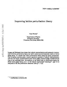
The structure of the full CI matrix is shown in Fig. 1. The matrix is real and symmetric, so that one can consider only the upper (or lower) triangular part of the matrix. The effective CI matrix is in the top-left corner of the full matrix and shown in black. The off-diagonal

3

N eff ~10

3

N s~10

of interest m,

6

E

0

FIG. 1: The structure of the CI matrix. The matrix is real and symmetric, therefore only upper triangular part is shown. Black triangular in the top left conner of the matrix is the effective CI matrix. Neglected off-diagonal matrix elements between high-energy states are shown in white.

matrix elements between high-energy states, which are put to zero, are shown in white. The diagonal matrix elements for the high-energy states are not neglected and shown in black. The off-diagonal matrix elements between low and high-energy states are shown in grey. The full CI matrix with this structure can be reduced to much smaller effective CI matrix with modified matrix elements hi|H CI |ji → hi|H CI |ji +

X hi|H CI |kihk|H CI |ji k

E (0) − Ek

.

(0i)

P 2 m cim Em = P . 2 m cim

(5)

The summation goes over all states of interest. Let us consider an example. We are interested in two low-energy states m = 1, 2, i.e. the sum in Eq. (5) contains only two terms. However, the state i may be any state from the group of the low-energy states P . We will need corresponding energy E (0i) in the calculation of the matrix element in the sum in Eq. (4). The energy E (0i) is close to those solutions Em of (2) where the basis state |ii contributes the most. Here we also need iterations over energies Em . However, only one run of the program is needed and all states come from the same matrix. The results for the energies are very close in both procedures. Note that the high-energy state corrections to the matrix elements of the effective CI matrix are similar to the second-order perturbation theory (PT) corrections to the energy. Therefore, we will use the corresponding CI and PT notations for the method. We test the assumptions (4) and (5) in Section IV by comparing the results of our CIPT method with exact diagonalization of the full CI matrix as shown in Fig. 1. The calculation of the sum over high-energy states (last term in (4)) takes up most of the computer time. However, the calculation of each term in this sum is independent of the others. This makes the method very convenient for parallel calculations. In next sections we describe in more detail specific calculations for atoms with open s, p, d and f shells and discuss the advantages and limitations of the suggested approach.

(4)

Here |ii ≡ Φi (r1 , . . . , rNe ), i, j ≤ Neff , Neff < k ≤ Ns , Ek = hk|H CI |ki, and E (0) is an initial approximation to the energy E in (2). In principle, the energies E in (2) and E (0) in (4) should be the same. However, since the energy is not known at this stage of the matrix calculation, one can perform iterations starting from some reasonable approximation for the energy and using the result of (2) for calculating matrix using (4) at the next iteration. If more than one state of definite J and parity is needed, the iterations should be done separately for each state. This leads to a couple of problems. First, too many runs of the program are needed to calculate several states of the same J and parity: the program becomes very inefficient. Second, different states of the same J π will correspond to different matrixes (4) which makes them non-orthogonal. This may lead to problems when calculating matrix elements between levels. We propose the following solution to both problems. The energy parameter E (0) in (4) is calculated for each basis state |ii according to its contribution to the states

III.

IODINE AND ITS IONS: LIMITS OF THE V N−M APPROXIMATION

The iodine atom and its ions are good subjects to study the limitations of the current approach based on reducing the size of the CI matrix and limitations of the V N −M approximation [45]. In the V N −M approximation the initial Hartree-Fock procedure is done for the N -electron atom with all M valence electrons removed. Then the CI technique is used to build the states of valence electrons. This works well when the overlap between core and valence states is small. Then the valence electrons have little effect on the core and the core is almost the same in the ion with all M valence electrons removed and in the neutral atom. This can be easily understood by considering the classical analog. If valence atomic electrons are approximated by a charged sphere with a hole inside, and all core electrons are inside this hole, then the charge sphere creates no electrical field inside it and thus has no effect on the internal electrons. This is usually the case when a new shell is started (with new principal quantum number n). In neutral atoms new shells always

4 TABLE I: Ground state energies (GSE) and ionization potentials for iodine and its ions from I VII to neutral I and corresponding numerical parameters used in the calculations. NNC is the number of the non-relativistic configurations included into the effective CI matrix, NRC and Neff are the corresponding numbers of relativistic configurations and configuration state functions (with given total angular momentum and parity), Ns is the total number of CSFs. Ns − Neff is the number of terms in the summation over high-energy states (see Eq. (4)). The ionization potential is calculated as a difference of the ground state energies of neighbouring ions. Ion/ Atom I VII I VI IV I IV I III I II II

Ground state Conf. Jπ 5s 1/2+ 5s2 0+ 2 5s 5p 1/2− 2 2 5s 5p 0+ 5s2 5p3 3/2− 5s2 5p4 2+ 2 5 5s 5p 3/2−

NNC

NRC

Neff

Ns

14 100 100 100 100 100 100

14 276 349 413 535 610 691

14 66 228 176 994 1551 1990

14 945 11092 18652 106287 168659 119490

start with s and p states. The ground state of neutral I is [Pd]5s2 5p5 . All core states have n < 5. So the overlap between 5s and 5p states and the core is small. Therefore, it can be considered in the V N −7 approximation. The iodine atom is an extreme case to check both the V N −M approximation and the CIPT method. It is the heaviest atom with an open p-shell for which the experimental spectrum is known. The only other heavier atom which has more external p-electrons, xenon, has no lowlying excited states. This means that the CIPT method is unlikely to work well for it: the expansion (1) for highly excited states will not be dominated by a small number of terms. The main advantage of using the V N −M approximation is relative simplicity of inclusion of the core-valence correlations [45]. They can be included using the lowest, second-order of the many-body perturbation theory [30], or single-double (SD) coupled-cluster method [29, 31], or all-order correlation potential method [46]. In this work we use the combination of the SD and CI methods developed in Ref. [31]. We use the V Z−7 approximation (N = Z for a neutral atom) and perform the calculations for all ions starting from the I VIII ion which has a closed-shell Pd-like core. The first ion for which we calculate excitation energies, the I VII ion, has only one valence electron. It is clear that the V Z−7 approximation is adequate for the I VII ion but deteriorates with increasing number of valence electrons. This is because the overlap between core and valence electrons is small but not exactly zero. It is instructive to estimate in advance what kind of uncertainty can be expected in neutral atoms due to the fact that the core is taken from the ion rather that from the neutral atom. For this purpose we have calculated the energy shift due to the difference of the core potential in the I VII ion and neutral iodine for the 5s and 5p electrons of I I. The results are h5s|δVcore |5si = 5055 cm−1 , h5p1/2 |δVcore |5p1/2 i = 3273 cm−1 , and h5p3/2 |δVcore |5p3/2 i = 2891 cm−1 . Total shift of the energy of the seven-electron ground state is ∼ 25000 cm−1 which is about 1% of the total removal

GSE (a.u.) -3.22403 -5.96185 -7.85009 -9.33862 -10.42426 -11.11511 -11.46144

IP (cm−1 ) CIPT NIST [1] 707590 706600(500) 600880 599800(3000) 414419 415510(300) 326693 325500(200) 238269 238500(200) 151623 154304.0(10) 76010 84295.1(2)

∆ 990 1080 -1090 1193 -230 -2680 -8285

energy. The contribution of this shift to the IP of neutral iodine is approximately equal to the energy shift of one 5p3/2 electron and constitutes about 3.5% of the IP. The effect on the excitation energies is expected to be smaller than 3000 cm−1 due to cancelation in energy shifts for low and upper states. Relative energy shifts for the ions is also small due to larger values of the energies. Next we compare the value of the energy shift due to the use of the V N −7 potential in neutral iodine with the contribution of the core-valence correlations. The total calculated removal energy for seven valence electrons of neutral iodine is -11.4614 a.u. (see Table I) when corevalence correlations are included. It comes to the value of -11.2225 a.u. when core-valence correlations are neglected. The difference, 0.2389 a.u. or 52430 cm−1 is about two times larger than the shift due to the use of the V N −7 potential (∼ 25000 cm−1 , see above). This justifies the use of the V N −M approximation for all iodine ions up to the neutral atom. Note that there is an alternative way of taking into account the core-valence correlations which does not require the removal of all valence electrons from initial approximation because their effect is included via the so-called subtraction diagrams [30]. The applicability of this approach to atoms with many valence electrons has never been properly studied. Table I presents calculated energies of the ground state for all iodine ions from I VII up to neutral I I. Ionization potentials of the ions are calculated as differences of the ground state energies of the neighbouring ions and compared with the data from the NIST database [1]. Relevant computational parameters are also presented. In all cases starting from I VI we include one hundred of the non-relativistic configurations (NNC) into the effective CI matrix. NRC and Neff are the corresponding numbers of the relativistic configurations and configuration state functions (CSFs), respectively. All other configurations are included perturbatively as a correction to the effective CI matrix according to formula (4). In the extreme cases of I II and I I the total number of CSFs (Ns ) is larger than the size of the effective CI matrix by about three

5 orders of magnitude. The difference between calculated IPs and those from the NIST databases is smaller than 0.4% for all cases apart from the extreme cases of I II and I I where its is 1.7% and about 10%, respectively. The deteriorating accuracy with increasing number of valence electrons is expected and most probably caused by insufficient size of the effective CI matrix and incompleteness of the many-electron basis states (e.g, triple and higher excitations are not included). Table II compares the calculated energy levels of iodine ions with experiment. In general the accuracy is good, about 1% or better for most of the states. However, we can see one more interesting tendency. The accuracy deteriorates not only with increased number of valence electrons but also with the increased excitation energy. This is also an expected effect. Highly excited states mix strongly with the high-energy states which are not included into the effective CI matrix and are only treated perturbatively. The accuracy for such states can be improved by increasing the size of the effective CI matrix. On the other hand, the accuracy for low-lying states is significantly better. Note that relatively poor accuracy for the 6s and 6p states of the I VII ion is due to a different reason which comes from the core-valence correlations. The energy parameter of the Σ1 operator which is responsible for the core-valence correlations is chosen to get best results for the lowest states, 5s and 5p (see, e.g. [30] for details).

IV.

TUNGSTEN ATOM

The tungsten atom is a good example of an atom with an open d-shell. Its ground state configuration is [Yb]5d4 6s2 . It has six valence electrons above the Yblike closed-shell core. This number is sufficiently large to make the full-scale CI calculations extremely difficult. On the other hand its spectrum is very well known. Therefore, the atom is good for checking the CIPT technique and demonstrating its use. The 5d valence electrons of W have relatively large overlap with the 5s and 5p core states which means that the V N −6 approximation would not work well for the atom (see Ref. [45] and the discussion in previous section). Therefore, we neglect core-valence correlations and use the V N −1 initial approximation. Note that choosing a good initial approximation is important for minimizing the size of the effective CI matrix, thus making the calculations more efficient. In full-scale CI calculations the choice of the initial approximation is less important and accuracy of the final results vary little from state to state regardless of their configurations. In our present approach most of basis states are included perturbatively and only very limited number of the lowest states are treated accurately via matrix diagonalization. Therefore, it is hardly possible to find an initial approximation which is equally good for states of all configurations. We may choose for example that the most important states

are those which belong to the 5d4 6s2 and 5d4 6s6p configurations to ensure high accuracy for the strong electric dipole transitions from the ground state. Then the V N −1 approximation in which one 6s electron is removed from initial self-consistent Hartree-Fock procedure seems to be an adequate choice. Indeed, all single-electron s, p, etc. states (including new 6s state) are calculated in the field of the frozen 5d4 6s core leading to the states of the 5d4 6snl configurations. The CIPT results for the W atom are presented in Table III. Calculations for even states were performed when only states of the 5d4 6s2 and 5d5 6s were included into the effective CI matrix, while all other states obtained by single and double excitations from these two configurations were included perturbatively. For odd states we used the 5d4 6s6p, 5d3 6s2 6p and 5d5 6p configurations as reference configurations to generate states for the effective CI matrix and for the PT expansion. For the tungsten case we also ran an exact diagonalization of the CI matrix shown in Fig. 1 using the AMBiT code (see, e.g. [32]); these are presented in the column “Full CI” of Table III. In this calculation, configuration state functions (CSFs) with definite J and parity are formed within each relativistic configuration (i.e. configurations formed in j-j electron coupling) and these are the basis functions for the CI procedure. We keep all matrix elements shown in black and grey in Fig. 1. In addition we keep all matrix elements between CSFs coming from the same relativistic configuration (these will appear close to the diagonal in the white section). We limit the storage to only the non-zero parts of the matrix and solve using the Davidson method [47] (implemented in [48]) which reduces diagonalization to a series of matrixvector multiplications. As an example, the J = 2 oddparity matrix size is Ns ≈ 3 × 106 but Neff = 144 only. We see in Table III that both solution of the Full CI and the CIPT method give good agreement with experiment. Comparison with diagonalization of the effective CI matrix without PT (the “Min. CI” column) shows that both methods give similar corrections to the level energies. This shows that the assumptions (4) and (5) are reasonable. Note the lower accuracy for the odd states (see Table III). Test calculations show that the accuracy can be further improved if more configurations are moved from the PT expansion to the effective CI matrix. This is a future direction for highly accurate calculations, however it takes a lot of computer power and is beyond the scope of this work.

V.

YTTERBIUM ATOM

The ytterbium atom has the [Ba]4f 14 6s2 closed-shell configuration in its ground state. However, the excited states of Yb belong to configurations which have excitations from both the 6s and 4f subshells. This means that a complete description of excited states of Yb is only pos-

6 TABLE II: Calculated excitation energies (CIPT, cm−1 ) of iodine and its ions, compared with experiment. Ion I VII

I VI

State 2

5s 5p 5p 5d 5d 6s 6p 6p 5s2 5s5p

5p2

5s5d

IV

5s2 5p 5s5p

2

5s2 5d 5s2 6s

S1/2 2 o P1/2 2 o P3/2 2 D3/2 2 D5/2 2 S1/2 2 o P1/2 2 o P3/2 1 S0 3 o P0 3 o P1 3 o P2 1 o P1 3 P0 3 P1 3 P2 1 D2 1 S0 3 D1 3 D2 3 D3 1 D2 2 o P1/2 2 o P3/2 4 P1/2 4 P3/2 4 P5/2 2 D3/2 2 D5/2 2 P1/2 2 P3/2 2 S1/2 2 D3/2 2 D5/2 2 S1/2

Expt. 0 104960 119958 274019 276256 335376 377185 382985 0 85666 89262 99685 127424 200085 208475 221984 209432 245659 251817 252540 253752 274162 0 12222 81018 85556 92558 108780 111831 125704 139398 138328 154050 155462 176814

Energy CIPT 0 105161 120229 274559 276802 337132 378800 384596 0 86140 89800 100345 126414 199827 208183 222252 209890 245657 251749 252262 253676 268727 0 12397 81417 87337 93108 109274 112498 124835 138098 138137 153666 155109 177614

∆ 0 -201 -271 -540 -546 -1756 -1615 -1611 0 -474 -538 -660 1010 258 292 -268 -458 2 68 278 76 5435 0 -175 -399 -1781 -550 -494 -667 869 1300 191 384 353 -802

Ion/ Atom I IV

State 5s2 5p2

5s5p3

I III

5s2 5p3

5s5p4

I II

5s2 5p4

5s2 5p3 6s 5s5p5

II

5s2 5p3 6s 5s2 5p5 5s2 5p4 6s

sible when the atom is treated as a system with sixteen valence electrons. There are many successful calculations in which Yb atom is treated as a two-valence electron system (see, e.g. [49–51]). In these calculations excitations are allowed only from the 6s2 subshell while the 4f electrons are attributed to the core. Good quality of the results indicate that the states with excitations from 6s and 4f subshells usually do not strongly mix. However, this is not always the case. There is at least one known case when the mixing is important. This is the mixing between the 4f 14 6s6p 1 Po1 state at E = 25068 cm−1 and the 4f 13 5d6s2 (7/2, 5/2)o1 state at E = 28857 cm−1 . The case is important due to the strong electric dipole tran-

3

P0 3 P1 3 P2 1 D2 1 S0 5 o S2 3 o D1 3 o D2 3 o D3 3 o P0 3 o P1 3 o P2 3 o S1 4 o S1/2 2 o D3/2 2 o D5/2 2 o P1/2 2 o P3/2 4 P5/2 4 P3/2 4 P1/2 2 D3/2 2 D5/2 3 P2 3 P0 3 P1 1 D2 1 S0 5 o S0 3 o P2 3 o P1 3 o P0 3 o S1 2 o P3/2 2 o P1/2 2 [2]5/2 2 [2]3/2 2 [0]1/2 2 [1]3/2 2 [1]1/2

Expt. 0 6828 10982 22532 37177 78084 99047 99542 102387 114658 115478 115013 135677 0 11711 14901 24299 29637 85555 90964 92902 103470 106619 0 6448 7087 13727 29501 81033 81908 84222 90405 84843 0 7603 54633 56093 60896 61820 61187

Energy CIPT 0 6909 11167 23004 37987 78495 99254 99853 102597 114702 115597 115040 133867 0 12149 14534 24640 30138 88539 93908 95820 110686 112931 0 6709 6910 14010 31955 88782 83765 96489 103475 87390 0 7311 64817 66762 72829 72508 75818

∆ 0 -81 -185 -472 -810 -411 -207 -311 -210 -44 -119 -27 1810 0 -438 367 -341 -501 -2984 -2944 -2915 -7216 -6312 0 -261 177 -283 -2454 -7749 -1857 -12267 -13070 -2547 0 -292 -10187 -10669 -11933 -10688 -14625

sition between ground and excited 4f 14 6s6p 1 Po1 state. It strongly dominates in the polarizability of Yb [49], it can be used in cooling [52], etc. The experimental value for the electric dipole amplitude is 4.148 a.u. while two-valence-electron calculations give the value of 4.825 a.u.; the difference is due to the mixing of the two odd states [49]. This mixing cannot be accounted for in the two-valence-electron calculations. Apart from studying the mixing it might be equally important to be able to get a complete description of the atomic spectrum including states with excitations from the core. This is especially useful when experimental data are incomplete or absent (e.g. superheavy elements

7 TABLE III: Calculated excitation energies (cm−1 ) of tungsten in different approximations. Min. CI: only leading configurations included (see text); Full CI: exact diagonalization with all configurations included, but off-diagonal matrix elements between CSFs outside the minimal CI set to zero; CIPT: diagonalisation of the effective CI with other configurations included in perturbation theory. ∆ is the difference between CIPT and experiment. Level 5d4 6s2

5

D

5d5 6s 5d4 6s2

7

S D

5d4 6s2 5d4 6s2 5d4 6s2 5d4 6s2 5d4 6s2 5d4 6s2

3

5d4 6s6p

7

Fo

5d4 6s2 5d5 6s

1 5

S2 P

5d4 6s6p 5d4 6s6p

7

5

Energy (cm−1 ) J Expt. [1] Min. CI Full CI CIPT 0 0 0 0 0 1 1670 776 1106 1502 3 2951 796 2494 2674 2 3325 1933 2740 2664 3 4830 3287 4272 4506 4 6219 4788 5509 5414 0 9528 13025 8530 9747 4 12161 14994 11730 12963 1 13307 16283 12078 13540 3 13348 16491 12916 14185 2 13777 17411 13030 14648 2 14976 18933 14144 15501 1 18082 21869 17171 18898 0 19389 4750 20303 20920 1 20064 5269 20927 21580 0 20174 25063 20255 20916 1 20427 28439 18965 20281 2 20983 25070 17692 22906 2 21448 6240 22090 22702 1 21453 7922 22199 23076

P2 H 3 P2 3 G 3 F2 3 D

3

7

Fo Do

∆ 0 168 277 661 324 805 -219 -802 -233 -837 -871 -525 -816 -1531 -1516 -742 146 -1923 -1254 -1623

TABLE IV: Calculated excitation energies (CIPT, cm−1 ) of ytterbium, compared with experiment. State 4f 14 6s2 4f 14 6s6p

1

S 3 o P

4f 13 5d6s2 4f 14 5d6s

(7/2,3/2)o 3 D

4f 14 6s6p 4f 14 5d6s 4f 13 5d6s2 4f 13 5d6s2 4f 13 5d6s2 4f 14 5d6s 4f 13 5d6s2 4f 13 5d6s2

1

Po D (7/2,3/2)o (7/2,5/2)o (7/2,3/2)o 1 D (7/2,3/2)o (7/2,5/2)o

3

J 0 0 1 2 2 1 2 1 3 5 6 3 2 4 2 1 4 3 5

Expt. [1] 0 17288 17992 19710 23188 24489 24751 25068 25270 25859 27314 27445 27677 28184 28195 28857 29774 30207 30524

Energy CIPT 0 17670 18305 19886 25028 27568 27217 25597 27747 26343 27205 27431 28071 28013 27354 30071 28975 29133 29172

∆ 0 -382 -331 -176 -1840 -3079 -2466 -529 -2477 -484 109 14 -394 171 841 -1214 799 1074 1352

and highly-charged ions). Yb atom is a good testing ground for developing appropriate approaches. It represents an extreme case of sixteen valence electrons while its experimental spectrum is very well known. As in the case of tungsten (see previous section) we start the calculations from the V N −1 approximation with one 6s electron removed from the self-consistent HartreeFock procedure. This leads to adequate treatment of the states of the 4f 14 6s2 and 4f 14 6s6p configurations while it is less adequate for the states of the 4f 13 5d6s2 configuration. The later can be compensated at least to some extend be increasing the size of the effective CI matrix. The results for Yb are presented in Table IV. Calculations for the ground state were performed with the inclusion of only two configurations to the effective CI matrix, the 4f 14 6s2 and the 4f 14 6s7s configurations. Even states with the total angular momentum J > 0 were calculated starting from the 4f 14 6s7s and the 4f 14 6s5d configurations. Odd states were calculated starting from the 4f 14 6s6p and the 4f 13 5d6s2 configurations. Accuracy of the results vary from state to state which should probably be expected for small-size CI matrix due to different convergence for states with different values of the total angular momentum J. We have seen similar features in the tungsten calculations (see previous section), however, for ytterbium it is more prominent. As in the case of tungsten, further significant improvement in accuracy can be achieved with increase of the size of the effective CI matrix. This would take greater computer power. Table V shows electric dipole (E1) transition amplitudes from the ground state of ytterbium to first four excited states that satisfy E1 selection rules. The calculations of the present work are done with the use of the random phase approximation (RPA) and CI wave functions as has been described in Ref. [49]. The CI wave function is taken from the calculations of the energies described above, i.e. it has sixteen valence electrons and includes excitations from the 4f subshell. The result for the h4f 14 6s6p 1 Po1 ||E1||4f 14 6s2 1 S0 i amplitude is in better agreement with the experiment than any other calculations. This is because present calculations include the mixing of the 4f 14 6s6p 1 Po1 and 4f 13 5d6s2 1 Po1 states while the other calculations treat the ytterbium atom as a two-valence-electron system and cannot include this mixing. It was noted in Ref. [49] that the calculation of the static dipole polarizability of Yb does not depend on the mixing of the 4f 14 6s6p 1 Po1 and 4f 13 5d6s2 (7/2, 5/2)o1 states if energy interval between them is neglected. This is because the sum of squares of the electric dipole matrix elements h4f 14 6s6p 1 Po1 ||E1||4f 14 6s2 1 S0 i2 + h4f 13 5d6s2 (7/2, 5/2)o1||E1||4f 14 6s2 1 S0 i2 does not depend on mixing. Therefore, it is instructive to compare the sum calculated in two different approximations. The sum is equal to 24.83 a.u. if the amplitudes calculated in present work are used (4.312 + 2.502 = 24.83,

8 TABLE V: Electric dipole transition amplitudes (reduced matrix elements) between ground and low excired states of Yb (a.u.) Upper state

Energy (cm−1 ) Expt. [1] CIPT 17992 18305

4f 14 6s6p 3 Po1

CIPT 0.763

4f 14 6s6p 1 Po1

25068

25597

4.31

4f 13 5d6s2 (7/2, 5/2)o1 4f 13 5d6s2 1 Po1

28857 37415

30071 37529

2.50 0.584

see Table V). The first amplitude calculated in the twovalence-electron approximation is equal to 4.825 a.u. [49]. The contribution of second state (4f 13 5d6s2 (7/2, 5/2)o1) to the polarizability is simulated by the contribution of the h4f7/2 ||E1||5d5/2 i matrix element into polarizability of atomic core. The value of this matrix element in the RPA approximation is equal to 1.40 a.u. The sum of squares of the two amplites is equal to 25.24 a.u. (4.8252 + 1.402 = 25.24). The two numbers (24.83 and 25.84) differ by only 1.6%. This illustrates the fact that the sum of squares of two amplitudes does not depend on mixing. In present work we include into the effective CI matrix mixing of the states with excitations from the 4f subshell, but we do not include mixing of the states with excitations from the 6s or 6p states. Therefore, we have good accuracy where the first mixing is more important and poor accuracy where the second mixing is more important. An example of the latter is the triplet state 4f 14 6s6p 3 Po1 ; the corresponding electric dipole matrix element is given to better accuracy by the two-valenceelectron calculations (see Table V).

VI.

DISCUSSION

The calculations for representative atoms with open p, d, and f -shells discussed above allow to come to some conclusions about the advantages and limitations of the new approach. The most obvious and important advantage is the ability to perform the calculations for any atom or ion regardless of the number of valence electrons. The calculations are totally ab initio with absolutely no fitting parameters. The same single-electron basis can be used for many-valence-electron atoms as has been used for few-valence-electron atoms (e.g., B-splines in a box [61]) in a number of calculations and has been proved to be complete. Another important advantage is huge gain in the efficiency compared with the full-scale CI calculations which can be achieved at the expense of little loss in accuracy by treating most of high-energy configurations perturbatively.

Amplitude Expt. 0.542(2) [53] 0.547(16) [55] 4.148(2) [57] 4.13(10) [58]

Other theory 0.54(8) [54] 0.587 [49] 0.41(1) [56] 4.825 [49] 4.40(80) [54] 4.44 [59] 4.89 [60]

The method is practically equivalent to the full-scale CI calculations for atoms or ions with few valence electrons (up to four or five). However, in contrast to the full-scale CI, it can be used for systems with any number of valence electrons, but with some limitations. For example, the calculations are sensitive to the choice of initial approximation. Since only limited number of states are included into the effective CI matrix and most of the states are treated perturbatively, it is important that the low-energy states are sufficiently close to the real physical states of interest and the contribution of the high-energy states is small. It is not always possible to find an approximation which is equally good for states of all low-lying configurations. For example, the V N −1 approximation for tungsten discussed above is good for the states of the 5d4 6s2 and 5d4 6snl configurations but it is less appropriate for the states of the 5d5 6s configuration. This may lead to different accuracy of the results for different states even when they belong to the same configuration. This is due to inaccurate treatment of the mixing with other configurations. The situation can be improved at the expense of using more computer power by increasing the size of the effective CI matrix. Another limitation comes from the fact that at present stage we cannot include core-valence correlations for systems with large number of valence electrons. This is not directly relevant to the approach considered in this work, however we mention it here because the ways of inclusion of the core-valence correlations for atoms with many valence electrons remains an open problem. The inclusion of the core-valence correlations is usually reduced to modification of the matrix element of the CI matrix [30] similar to what is done here for inclusion of high-energy states (see Eq. (4)). However, our current approach presents a way of reducing the size of the CI matrix regardless of the origin of its matrix elements, i.e. regardless of whether core-valence correlations are included or not, what kind of basis is used, etc. In Section III we considered an extreme case of the seven-valence-electron atom, iodine. The core-valence correlations were included and the V N −7 approximation was used for this purpose. This approach would not work for tungsten or ytterbium or any other atom with large number of valence electrons.

9 Funding more suitable approaches is a subject for further study. VII.

CONCLUSION

We present a version of the CI method which treats high-energy many-electron basis states perturbatively, hugely reducing the size of the CI matrix. In principle, the method can work for systems with any number of valence electrons. Calculations for iodine and its ions, tungsten, and ytterbium (atoms with open p, d, and f shells) show that good accuracy for the energies can be achieved for wide range of atomic systems. The method is equivalent to the full-scale CI method for systems with

[1] A. Kramida, Yu. Ralchenko, J. Reader, and and NIST ASD Team, NIST Atomic Spectra Database (ver. 5.3), [Online]. Available: http://physics.nist.gov/asd [2016, January 11]. National Institute of Standards and Technology, Gaithersburg, MD. (2015). [2] F. P. Hessberger, ChemPhysChem 14, 483 (2013). [3] A. T¨ urler and V. Pershina, Chem. Rev. 113, 1237 (2013). [4] J. H. Hamilton, S. Hofmann, and Y. T. Oganessian, Annu. Rev. Nucl. Part. Sci. 63, 383 (2013). [5] J. C. Berengut, V. A. Dzuba, and V. V. Flambaum, Phys. Rev. Lett. 105, 120801 (2010). [6] J. C. Berengut, V. A. Dzuba, V. V. Flambaum, and A. Ong, Phys. Rev. Lett. 106, 210802 (2011). [7] J. C. Berengut, V. A. Dzuba, V. V. Flambaum, and A. Ong, Phys. Rev. Lett. 109, 070802 (2012). [8] J. C. Berengut, V. A. Dzuba, V. V. Flambaum, and A. Ong, Phys. Rev. A 86, 022517 (2012). [9] V. A. Dzuba, V. V. Flambaum, and H. Katori, Phys. Rev. A 91, 022119 (2015). [10] M. S. Safronova, V. A. Dzuba, V. V. Flambaum, U. I. Safronova, S. G. Porsev, and M. G. Kozlov, Phys. Rev. Lett. 113, 030801 (2014). [11] M. S. Safronova, V. A. Dzuba, V. V. Flambaum, U. I. Safronova, S. G. Porsev, and M. G. Kozlov, Phys. Rev. A 90, 042513 (2014). [12] M. S. Safronova, V. A. Dzuba, V. V. Flambaum, U. I. Safronova, S. G. Porsev, and M. G. Kozlov, Phys. Rev. A 90, 052509 (2014). [13] V. A. Dzuba and V. V. Flambaum, Hyperfine Interactions 236, 79 (2015). [14] T. Pruttivarasin, M. Ramm, S. G. Porsev, I. I. Tupitsyn, M. S. Safronova, M. A. Hohensee, and H. Haffner, Nature(London) 517, 592 (2015). [15] V. A. Dzuba, V. V. Flambaum, M. S. Safronova, S. G. Porsev, T. Pruttivarasin, M. A. Hohensee, and H. H¨ affner, Nat. Phys. (2016). [16] K. VanTilburg, N. Leefer, L. Bougas, and D. Budker, Phys. Rev. Lett. 115, 011802 (2015). [17] Y. V. Stadnik and V. V. Flambaum, Phys. Rev. Lett. 113, 151301 (2014). [18] A. Derevianko and M. Pospelov, Nat. Phys. 10, 933 (2014). [19] Y. V. Stadnik and V. V. Flambaum, Phys. Rev. Lett. p.

few valence electrons (up to four or five). The accuracy for the energies for such systems is on the level of 1% in both approaches. However, the new approach is much more efficient for systems where full-scale CI calculations are difficult (four or five valence electrons). The accuracy for the energies of atoms or ions with large number of valence electrons (up to sixteen) is on the level of few per cent and can be controlled by varying the size of the effective CI matrix. Acknowledgments

The work was supported in part by the Australian Research Council.

to be published (2015). [20] A. Derevianko, V. A. Dzuba, and V. V. Flambaum, Phys. Rev. Lett. 109, 180801 (2012). [21] V. A. Dzuba, A. Derevianko, and V. V. Flambaum, Phys. Rev. A 86, 054501 (2012). [22] V. A. Dzuba, A. Derevianko, and V. V. Flambaum, Phys. Rev. A 87, 029906(E) (2013). [23] R. D. Cowan, The Theory of Atomic Structure and Spectra (University of California Press, Berkeley and Los Angeles, 1981). [24] U. I. Safronova, W. R. Johnson, and J. R. Albritton, Phys. Rev. A 62, 052505 (2000). [25] V. A. Dzuba, V. V. Flambaum, and O. P. Suskov, Phys. Lett. A 140, 493 (1989). [26] R. Pal, M. S. Safronova, W. R. Johnson, A. Derevianko, and S. G. Porsev, Phys. Rev. A 75, 042515 (2007). [27] E. Eliav, M. J. Vilkas, Y. Ishikawa, and U. Kaldor, Chem. Phys. 311, 163 (2005). [28] P. J¨ onsson, G. Gaigalas, J. Biero´ n, C. F. Fischer, and I. P. Grant, Comp. Phys. Comm. 184, 2197 (2013). [29] M. S. Safronova, M. G. Kozlov, W. R. Johnson, and D. Jiang, Phys. Rev. A 80, 012516 (2009). [30] V. A. Dzuba, V. V. Flambaum, and M. G. Kozlov, Phys. Rev. A 54, 3948 (1996). [31] V. A. Dzuba, Phys. Rev. A 90, 012517 (2014). [32] J. C. Berengut, V. V. Flambaum, and M. G. Kozlov, Phys. Rev. A 73, 012504 (2006). [33] J. C. Berengut, Phys. Rev. A 94, 012502 (2016). [34] M. Block (2015), talk on the Pacifichem 2015 Congress, Honolulu. [35] M. Laatiaoui, W. Lauth, H. Backe, M. Block, D. Ackermann, B. Cheal, P. Chhetri, C. E. Dllmann, P. van Duppen, J. Even, et al., Nature 538, 495 (2016). [36] T. Sato (2015), talk on the Pacifichem 2015 Congress, Honolulu. [37] T. Sato, M. Asai, A. Borschevsky, T. Stora, N. Sato, Y. Kaneya, K. Tsukada, C. E. D¨ ullmann, K. Eberhardt, E. Eliav, et al., Nature 520, 209 (2015). [38] A. Windberger, J. R. C. Lopez-Urrutia, H. Bekker, N. S. Oreshkina, J. C. Berengut, V. Bock, A. Borschevsky, V. A. Dzuba, E. Eliav, Z. Harman, et al., Phys. Rev. Lett. 114, 150801 (2015). [39] T. Nakajima, K. Okada, M. Wada, V. A. Dzuba, M. S.

10

[40] [41] [42] [43] [44] [45] [46] [47] [48] [49] [50] [51]

Safronova, U. I. Safronova, N. Ohmae, H. Katori, and N. Nakamura (2016), to be published. V. A. Dzuba and V. V. Flambaum, Phys. Rev. A 77, 012514 (2008). V. A. Dzuba and V. V. Flambaum, Phys. Rev. A 77, 012515 (2008). A. Landau, E. Eliav, Y. Ishikawa, and U. Kaldor, J. Chem. Phys. 115, 6862 (2001). I. M. Savukov, W. R. Johnson, and H. G. Berry, Phys. Rev. A 66, 052501 (2002). V. A. Dzuba and V. V. Flambaum, Phys. Rev. Lett. 104, 213002 (2010). V. A. Dzuba, Phys. Rev. A 71, 032512 (2005). J. S. M. Ginges and V. A. Dzuba, Phys. Rev. A 91, 042505 (2015). E. R. Davidson, J. Comp. Phys. 17, 87 (1975). A. Stathopoulos and C. F. Fischer, Comp. Phys. Comm. 79, 268 (1994). V. A. Dzuba and A. Derevianko, J. Phys. B 43, 074011 (2010). S. G. Porsev, Y. G. Rakhlina, and M. G. Kozlov, J. Phys. B 32, 1113 (1999). M. S. Safronova, S. G. Porsev, and C. W. Clark, Phys.

Rev. Lett. 109, 230802 (2012). [52] T. Kobayashi, D. Akamatsu, Y. Nishida, and et al., Optics Express 24, 2142 (2016). [53] K. Beloy, J. A. Sherman, N. D. Lemke, N. Hinkley, C. W. Oates, and A. D. Ludlow, Phys. Rev. A 86, 051404(R) (2012). [54] S. G. Porsev, Y. G. Rakhlina, and M. G. Kozlov, Phys. Rev. A 60, 2781 (1999). [55] C. J. Bowers, D. Budker, E. D. Commins, D. DeMille, S. J. Freedman, A.-T. Nguyen, S.-Q. Shang, and M. Zolotorev, Phys. Rev. A 53, 3103 (1996). [56] K. Guo, G. Wang, and A. Ye, J. Phys. B 43, 135004 (2010). [57] Y. Takasu, K. Komori, K. Honda, M. Kumakura, T. Yabuzaki, and Y. Takahashi, Phys. Rev. Lett. 93, 123202 (2004). [58] M. Baumann and G. Wandel, Phys. Rev. Lett. 22, 283 (1966). [59] J. Migdalek and W. E. Baylis, J. Phys. B 24, L99 (1991). [60] M. D. Kunisz, Acta Phys. Pol. A 62, 285 (1982). [61] W. R. Johnson and J. Sapirstein, Phys. Rev. Lett. 57, 1126 (1986).