This limits EKF-SLAM to environments suited to such models and tends to
discard much ... The resulting Scan-SLAM combines the general applicabil- ity of
scan ...
1 Scan-SLAM: Combining EKF-SLAM and Scan Correlation Juan Nieto, Tim Bailey and Eduardo Nebot ARC Centre of Excellence for Autonomous Systems (CAS) The University of Sydney, NSW, Australia {j.nieto,tbailey,nebot}@acfr.usyd.edu.au Summary. This paper presents a new generalisation of simultaneous localisation and mapping (SLAM). SLAM implementations based on extended Kalman filter (EKF) data fusion have traditionally relied on simple geometric models for defining landmarks. This limits EKF-SLAM to environments suited to such models and tends to discard much potentially useful data. The approach presented in this paper is a marriage of EKF-SLAM with scan correlation. Instead of geometric models, landmarks are defined by templates composed of raw sensed data, and scan correlation is shown to produce landmark observations compatible with the standard EKF-SLAM framework. The resulting Scan-SLAM combines the general applicability of scan correlation with the established advantages of an EKF implementation: recursive data fusion that produces a convergent map of landmarks and maintains an estimate of uncertainties and correlations. Experimental results are presented which validate the algorithm.
Key words: Simultaneous localisation and mapping (SLAM), EKF-SLAM, scan correlation, Sum of Gaussians (SoG), observation model
1.1 Introduction A mobile robot must know where it is within an environment in order to navigate autonomously and intelligently. Self-location and knowing the location of other objects requires the existence of a map, and this basic requirement has lead to the development of the simultaneous localisation and mapping (SLAM) algorithm over the past two decades, where the robot builds a map piece-wise as it explores the environment. The predominant form of SLAM to date is stochastic SLAM as introduced by Smith, Self and Cheeseman [11]. Stochastic SLAM explicitly accounts for the errors that occur in sensed measurements: measurement errors introduce uncertainties in the location estimates of map landmarks which, in turn, incur uncertainty in the robot location estimate, and so the landmark and robot pose estimates are dependent. Practical implementations of stochastic SLAM represent these uncertainties and correlations
2
Juan Nieto, Tim Bailey and Eduardo Nebot
with a Gaussian probability density function (PDF), and propagate the uncertainties using an extended Kalman filter (EKF). This form of SLAM is known as EKF-SLAM [6]. One problem with EKF-SLAM is that requires the sensed data to be modelled as geometric shapes, which limits the approach to environments suited to such models. This paper presents a new approach to SLAM which is based on the integration of scan correlation methods with the EKF-SLAM framework. The map is constructed as an on-line data fusion problem and maintains an estimate of uncertainties in the robot pose and landmark locations. There is no requirement to accumulate a scan history. Unlike previous EKF-SLAM implementations, landmarks are not represented by simplistic geometric models, but rather are defined by a template of raw sensor data. This way the feature models are not environment specific and good data is not thrown away. The result is Scan-SLAM that uses raw data to represent landmarks and scan matching to produce landmark observations. In essence, this approach presents a new way to define generic observation models, and in all other respects Scan-SLAM behaves in the manner of conventional EKF-SLAM. The format of this paper is as follows. The next section presents a review of related work. Section 1.3 describes a sum of Gaussians (SoG) representation for scans of range-bearing data, based on the work presented in [1, Chapter 4]. Section 1.4 presents a method for obtaining a Gaussian likelihood function from the scan correlation procedure, which produces an observation in a form compatible with EKF-SLAM. Section 1.5 describes the generic observation model that is applied to all feature observations obtained by scan correlation. Section 1.6 presents Scan-SLAM, which uses the developments of Sections 1.4 and 1.5 to implement a scan correlation based observation update step within the EKF-SLAM framework. The method is validated with experimental results. Finally, conclusions are presented in Section 1.8.
1.2 Related Work A significant issue with EKF-SLAM [4] is the design of the observation model. Current implementations require landmark observations to be modelled as geometric shapes, such as lines or circles. Measurements must fit into one of the available geometric categories in order to be classified as a feature, and non-conforming data is ignored. The chief problem with geometric observation models is that they tend to be environment specific, so that a model suited to one type of environment might not work well in another and, in any case, a lot of useful data is thrown away. An alternative to geometric feature models is a procedure called scan correlation, which computes a maximum likelihood alignment between two sets of raw sensor data. Thus, given a set of observation data and a reference map composed similarly of unprocessed data points, a robot can locate itself without converting the measurements to any sort of geometric primitive. The
1 Scan-SLAM: Combining EKF-SLAM and Scan Correlation
3
observations are simply aligned with the map data so as to maximise a correlation measure. Scan correlation has primarily been used as a localisation mechanism from an a priori map [13, 8, 3, 9], with the iterated closest point (ICP) algorithm [2, 10] and occupancy grid correlation [5] being the most popular correlation methods. Two significant methods have been presented that perform scan correlation based SLAM. The first [12] uses expectation maximisation (EM) to maximise the correlation between scans, which results in a set of robot pose estimates that give an “optimal” alignment between all scans. The second method [7] accumulates a selected history of scans, and aligns them as a network. This approach is based on the algorithm presented in [10]. The main concern with these methods is that they do not perform data fusion, instead requiring a (selected) history of raw scans to be stored, and they are not compatible with the traditional EKF-SLAM formulation. This paper presents a new algorithm that combines EKF-SLAM with scan correlation methods.
1.3 Scan Matching using Gaussian Sum Representation A set of point measurements may be represented as a sum of Gaussians. This representation permits efficient correlation of two scans of data, and has a Bayesian justification which ensures that, under certain conditions, the scan alignment estimate is consistent (see [1]). SoG correlation also avoids limitations inherent to occupancy grid and ICP correlation methods; these being fixed-scale granularity and point-to-point data associations, respectively. For a set of range-bearing measurements, such as a range-laser scan, the measurements and their uncertainties are first converted to sensor-centric Cartesian space. That is, a range-bearing measurement zi = (ri , θi ) with Gaussian uncertainty Ri , is converted to Cartesian coordinates � � r cos θi xi = f (zi ) = i ri sin θi Pi = ∇fzi Ri ∇fzTi ∂f where the Jacobian ∇fzi = ∂z . i We define an n-dimensional Gaussian as � � 1 1 ¯ )T P−1 (x − p ¯) ¯ , P) , p exp − (x − p g(x; p 2 (2π)n |P|
¯ and P are the mean and covariance, respectively. An n-dimensional where p sum of Gaussians (SoG) is defined as the sum of k scaled Gaussians. G(x) ,
k X i=1
¯ i , Pi ) αi g(x; p
4
Juan Nieto, Tim Bailey and Eduardo Nebot 4
3
2
metres
1
0
−1
−2
−3
−4
−5 −1
0
1
2
3
4
5
6
7
8
metres
Fig. 1.1. The left-hand figure shows the set of raw range-laser data points transformed to a sensor-centric coordinate frame. The right-hand figure shows the SoG representation of this scan.
where, for a normalised SoG, the sum of the scaling factors αi is one. However, normalisation is not necessary for correlation purposes—only relative scale is important—and it is more convenient to work with non-normalised SoGs. An example of a SoG produced from a range-laser scan is shown in Fig. 1.1. Given two scans of Cartesian data points, where each point has a mean and variance, the respective scans may be represented by two SoGs. G1 (x) =
k1 X
¯ i , Pi ) αi g(x; p
k2 X
¯ i , Qi ) βi g(x; q
i=1
G2 (x) =
i=1
A likelihood function for the correlation of these two SoGs is given by their cross-correlation. Λ(x) = G1 (x) ? G2 (x) Z X k1 k2 X ¯ i , Pi ) ¯ j , Qj )du = αi g(u − x; p βj g(u; q i=1
=
k1 X k2 X
j=1
αi βj γij (x)
(1.1)
i=1 j=1
¯ i , Pi ) and g(x; q ¯ j , Qj ). where γij (x) is the cross-correlation of two Gaussians g(x; p � � 1 1 exp − (x − µ ¯)T Σ−1 (x − µ ¯) γij (x) = p n 2 (2π) |Σ|
1 Scan-SLAM: Combining EKF-SLAM and Scan Correlation
5
¯i − q ¯j µ ¯=p Σ = Pi + Qj The result is a likelihood function that provides a measure of scan alignment, and a maximum-likelihood alignment can be obtained as xM = arg max Λ(x) x
(1.2)
where pose xM is the maximum-likelihood location of scan 1 with respect to scan 2. More precisely, xM is the location of the coordinate frame of scan 1 with respect to the coordinate frame of scan 2. Full details of Gaussian sum correlation can be found in [1, Section 4.4]. In particular, it describes SoG scaling factors, SoG correlation in a plane (with alignment over position and orientation), and various alternatives for efficient implementation.
1.4 Scan Correlation Variance For scan correlation to be compatible with EKF-SLAM, it is necessary to approximate the correlation likelihood function in (1.1) by a Gaussian. This section presents a method to compute a mean and variance for scan correlation based on the shape of the likelihood function in the vicinity of the point of maximum-likelihood. The resulting approximation is reasonable because the likelihood function tends to be Gaussian in shape in the region close to the maximum-likelihood. The first step in deriving this approximation is to compute the variance of a Gaussian function given only a set of point evaluations of the function. Given a Gaussian PDF � � 1 1 T −1 ¯ ) P (x − p ¯) ¯ , P) = p exp − (x − p g(x; p 2 (2π)n |P|
the maximum-likelihood value is found at its mean ¯ , P) = p g(¯ p; p
1 (2π)n |P|
= CM
Any other sample xi from this distribution will have the value � � 1 T −1 ¯ ) P (xi − p ¯) ¯ , P) = CM exp − (xi − p g(xi ; p 2 = Ci By taking logs and rearranging terms, we get ¯ )T P−1 (xi − p ¯ ) = −2(ln Ci − ln CM ) (xi − p
(1.3)
6
Juan Nieto, Tim Bailey and Eduardo Nebot
Thus, given a set of samples {xi } and their associated function evaluations ¯ and CM , then the {Ci }, along with the maximum-likelihood parameters p inverse covariance matrix P−1 (and hence P) can be evaluated. The only requirement is that the number of samples equals the number of unknown elements in P−1 . In this paper, we are concerned with 3-dimensional Gaussians, (i.e., to represent the distribution of a landmark pose [xL , yL , φL ]T ), and so we present the full derivation of variance evaluation for this case. We define the following variables 0
Ci = −2(ln Ci − ln CM ) ¯ = [xi , yi , zi ]T xi − p ab c P−1 = b d e cef Substituting these into (1.3) and expanding terms gives 0
x2i a + 2xi yi b + 2xi zi c + yi2 d + 2yi zi e + zi2 f = Ci
(1.4)
The result is an equation with six unknowns (a, . . . , f ), and so a solution can be found given six samples from the Gaussian. This is posed as a matrix equation of the form Ax = b where the i-th row of A is [x2i , 2xi yi , 2xi zi , yi2 , 2yi zi , zi2 ], x is the unknowns 0 [a, b, c, d, e, f ]T , and b is the set of solutions {Ci }. For a Gaussian function, the solution of this system of equations gives the exact covariance matrix of the function. Since the scan correlation likelihood function is not exactly Gaussian (although we presume it has approximately Gaussian shape near the maximum likelihood location), different sets of samples will produce different values for P. To reduce this variation, we evaluate more than the minimum number of samples and compute a least-squares solution using singular value decomposition (SVD), which results in a much more stable covariance estimate. In summation, two SoGs are aligned according to a maximum likelihood correlation, to give the pose xM between scan coordinate frames. A number of samples, N > 6, from the region near xM are evaluated and the alignment variance PM is computed by SVD. At a higher level of abstraction, the result of this algorithm can be described by the following pseudocode function interface [xM , PM ] = scan_align(G1 (x),G2 (x), x0 ) where x0 is an initial guess of the pose of G1 (x) relative to G2 (x). A good initial pose is required to promote reliable convergence.
1 Scan-SLAM: Combining EKF-SLAM and Scan Correlation
7
1.5 Generic Observation Model We define a landmark by a SoG in a local landmark coordinate frame, and the Scan-SLAM map stores a global pose estimate of this coordinate frame in its state vector (see Section 1.6 for details). Thus, all observations of landmarks obtained by scan matching can be modelled as the measurement of a global landmark frame xL as seen from the global vehicle pose xv (see Fig. 1.2). The generic observation model for the pose of a landmark coordinate frame with respect to the vehicle is as follows. z = [xδ , yδ , φδ ]T = h (xL , xv ) (xL − xv ) cos φv + (yL − yv ) sin φv = −(xL − xv ) sin φv + (yL − yv ) cos φv φL − φv
(1.5)
1.6 Scan-SLAM Update Step When an object is observed for first time, a new landmark is created. A landmark definition template is created by extracting from the current scan the set of measurements that observe the object. These measurements form a SoG, which is transformed to a coordinate frame local to the landmark. While there is no inherent restriction as to where this local axis is defined, it is more intuitive to locate it somewhere close to the landmark data-points and, in this paper, we define the local coordinate frame as the centroid of the template SoG. A new landmark is added to the SLAM map by adding the global pose of its coordinate frame to the SLAM state vector. Note that the landmark description template is not added to the SLAM state and is stored in a separate data structure. As new scans become available, the SLAM estimate of existing map landmarks can be updated by the following process. First, the location of a map
Fig. 1.2. All SoG features are represented in the SLAM map as a global pose identifying the location of the landmark coordinate frame. The generic observation model for these features is a measurement of the global landmark pose xL with respect to the global vehicle pose xv . The vehicle-relative observation is z = [xδ , yδ , φδ ]T .
8
Juan Nieto, Tim Bailey and Eduardo Nebot
landmark relative to the vehicle is predicted to determine whether the landmark template SoG GL (x) is in the vicinity of the current scan SoG Go (x). ˆ according This vehicle-relative landmark pose is the predicted observation z to (1.5). If the predicted location is sufficiently close to the current scan, the landmark template is aligned with the scan using the SVD correlation algoˆ as an initial guess (see Fig. 1.3). rithm, using z ˆ) [z, R] = scan_align(GL (x), Go (x), z The result of scan alignment gives the pose of the landmark template frame with respect to the current scan coordinate frame, which is defined by the current vehicle pose. This is the new landmark observation z with uncertainty R, in accordance with the generic observation model in (1.5). Having obtained the observation z and R, the SLAM state is updated in the usual manner of EKF-SLAM.
Fig. 1.3. The top figure shows a stored scan landmark template (solid line) and a new observed scan (dashed line). The bottom figure shows the scan alignment evaluated with the scan correlation algorithm from which the observation vector z is obtained.
1.7 Results This section presents simulation and experimental results of the algorithm presented. The importance of the simulation results is in the possibility to compare the actual objects position with the estimated by Scan-SLAM. Fig. 1.4 shows the simulation environment. The experiment was done in a large area of 180 by 160 metres with a sensor field of view of 30 metres. The vehicle travels at a constant speed of 3m/s. The sensor observations are corrupted with Gaussian noise with standard deviations 0.1 metres in range and 1.5 degrees in bearing. The simulation map consists of objects with different geometry and size. In order to select the segments to be added into
1 Scan-SLAM: Combining EKF-SLAM and Scan Correlation
9
the navigation map, a basic segmentation algorithm was implemented that selects sensor segments that contain a minimum number of neighbour points. The results for the Scan-SLAM algorithm are shown in Fig. 1.4. Here the solid line depicts the ground truth for the robot pose and the dashed line the estimated vehicle path. The actual object’s position is represented by the light solid line and the segment’s position by the dark points. The local axis pose for each scan landmark is also shown and the ellipses indicate the 3σ uncertainty bound of each scan landmark. The local axis position was defined equal to the average position of the raw points included in the segment and the orientation equal to the vehicle orientation. Fig. 1.5 shows the result after the vehicle closes the loop and the EKF-SLAM updates the map. The alignment between the actual object’s position and that estimated by the algorithm after closing the loop can be observed.
60
40
metres
20
0
−20
−40
−60 −80
−60
−40
−20
0 metres
20
40
60
80
Fig. 1.4. The figure shows the simulation environment. The solid line depicts the ground truth for the robot pose and the dashed line the estimated vehicle path. The actual object positions are represented by the light solid line and the segment positions by the dark points. The ellipses indicate the 3σ uncertainty bound of each scan landmark.
The algorithm was also tested using experimental data. In the experiment a standard utility vehicle was fitted with dead reckoning and laser range sensors. The testing environment was the car park near the ACFR building. The environment is mainly dominated by buildings and trees. Fig. (1.6) illustrates the result obtained with the algorithm. The solid line denotes the trajec-
10
Juan Nieto, Tim Bailey and Eduardo Nebot 60
40
metres
20
0
−20
−40
−60 −80
−60
−40
−20
0 metres
20
40
60
80
Fig. 1.5. Simulation result after closing the loop.
tory estimated. The light points is a laser-image obtained using feature-based SLAM and GPS, which can be used as a reference. The dark points represent the template scans and the ellipses the 1σ covariance bound. The local axis for the scan landmarks were also drawn in the figure. The segmentation criterion was also based on distance. Seven scan landmarks were incorporated and used for the SLAM.
1.8 Conclusions and Future Work EKF-SLAM is currently the most popular filter used to solve stochastic SLAM. An important issue with EKF-SLAM is that it requires sensory information to be modelled as geometric shapes and the information that does not fit in any of the geometric models is usually rejected. On the other hand, scan correlation methods use raw data and are not restricted to geometric models. Scan correlation methods have mainly be used for localisation given an a priori map. Some algorithms that perform scan correlation based SLAM have appeared, but they do not perform data fusion and they require storage of a history of raw scans. The Scan-SLAM algorithm presented in this paper combines scan correlation with EKF-SLAM. The hybrid approach uses the best of both paradigms; it incorporates raw data into the map representation and so does not require geometric models, and estimates the map in a recursive manner without the
1 Scan-SLAM: Combining EKF-SLAM and Scan Correlation
11
50
40
North(metres)
30
20
10
0
−10
−20
−30 −40
−30
−20
−10
0 10 East(metres)
20
30
40
Fig. 1.6. Scan-SLAM result obtained in the car park area. The solid line denotes the trajectory estimated. The light points is a laser-image obtained using feature-based SLAM and GPS. The dark points represent the template scans and the ellipses the 1σ covariance bound.
need to store the scan history. It works as an EKF-SLAM that uses raw data as landmarks and utilises scan correlation algorithms to produce landmark observations. Finally experimental results were presented that showed the efficacy of the new algorithm. In terms of future research, there is a lot of scope for developing the data association capabilities that arise from combining scan correlation with EKFSLAM metric constraints. The ability of batch data association within an EKF framework to reject spurious data is well developed (e.g., [1, Chapter 3]). Scan correlation has the potential to strengthen the rejection of outliers by matching consecutive sequences of scans and removing points that are not reobserved. Also, scan correlation provides a measure of how well the shape of one scan fits another and can reject associations that have compatible metric constraints but misfitting shape. A second area for future work is the development of continuously improving landmark templates. As a landmark is reobserved, perhaps from different view-points, the template model that describes it can be refined to better represent the object.
12
Juan Nieto, Tim Bailey and Eduardo Nebot
Acknowledgments This work is supported by the ARC Centre of Excellence programme, funded by the Australia Research Council (ARC) and the New South Wales State Government.
References 1. T. Bailey. Mobile Robot Localisation and Mapping in Extensive Outdoor Environments. PhD thesis, University of Sydney, Australian Centre for Field Robotics, 2002. 2. P.J. Besl and N.D. McKay. A method for registration of 3-D shapes. IEEE Transactions on Pattern Analysis and Machine Intelligence, 14(2):239–256, 1992. 3. W. Burgard, A. Derr, D. Fox, and A.B. Cremers. Integrating global position estimation and position tracking for mobile robots: The dynamic markov localization approach. In IEEE/RSJ International Conference on Intelligent Robots and Systems, 1998. 4. M.W.M.G. Dissanayake, P. Newman, S. Clark, H.F. Durrant-Whyte, and M. Csorba. A solution to the simultaneous localization and map building (SLAM) problem. IEEE Transactions on Robotics and Automation, 17(3):229– 241, 2001. 5. A. Elfes. Occupancy grids: A stochastic spatial representation for active robot perception. In Sixth Conference on Uncertainty in AI, 1990. 6. J. Guivant and E. Nebot. Optimization of the simultaneous localization and map building algorithm for real time implementation. IEEE Transactions on Robotics and Automation, 17(3):242–257, 2001. 7. J.S. Gutmann and K. Konolige. Incremental mapping of large cyclic environments. In IEEE International Symposium on Computational Intelligence in Robotics and Automation, pages 318–325, 1999. 8. J.S. Gutmann and C. Schlegel. Amos: Comparison of scan matching approaches for self-localization in indoor environments. In 1st Euromicro Workshop on Advanced Mobile Robots (Eurobot’96), pages 61–67, 1996. 9. K. Konolige and K. Chou. Markov localization using correlation. In International Joint Conference on Articial Intelligence, pages 1154–1159, 1999. 10. F. Lu and E. Milios. Robot pose estimation in unknown environments by matching 2D range scans. Journal of Intelligent and Robotic Systems, 18:249–275, 1997. 11. R. Smith, M. Self, and P. Cheeseman. A stochastic map for uncertain spatial relationships. In Fourth International Symposium of Robotics Research, pages 467–474, 1987. 12. S. Thrun, W. Bugard, and D. Fox. A real-time algorithm for mobile robot mapping with applications to multi-robot and 3D mapping. In International Conference on Robotics and Automation, pages 321–328, 2000. 13. G. Weiß, C. Wetzler, and E. Puttkamer. Keeping track of position and orientation of moving indoor systems by correlation of range-finder scans. In International Conference on Intelligent Robots and Systems, pages 595–601, 1994.