Combining Estimators. Bias-variance decomposition. If we could average over all possible datasets, let the average prediction be. The average prediction error ...
Combining Estimators to Improve Performance A survey of “model bundling” techniques -from boosting and bagging, to Bayesian model averaging -- creating a breakthrough in the practice of Data Mining.
John F. Elder IV, Ph.D. Elder Research, Charlottesville, Virginia www.datamininglab.com Greg Ridgeway, Ph.D. University of Washington, Dept. of Statistics www.stat.washington.edu/greg © 1999 Elder & Ridgeway
KDD99 T5-1
Combining Estimators
Outline • Why combine? A motivating example • Hidden dangers of model selection • Reducing modeling uncertainty through Bayesian Model Averaging • Stabilizing predictors through bagging • Improving performance through boosting • Emerging theory illuminates empirical success • Bundling, in general • Latest algorithms • Closing Examples & Summary © 1999 Elder & Ridgeway
KDD99 T5-2
Combining Estimators
Reasons to combine estimators • Decreases variability in the predictions. • Accounts for uncertainty in the model class. P−> Improved accuracy on new data.
© 1999 Elder & Ridgeway
KDD99 T5-3
Combining Estimators
A Motivating Example: Classifying a bat’s species from its chirp • Goal: Use time-frequency features of echolocation signals to classify bats by species in the field (avoiding capture and physical inspection). • U. Illinois biologists gathered data: 98 signals from 19 bats representing 6 species: Southeastern, Grey, Little Brown, Indiana, Pipistrelle, Big-Eared. • ~35 data features (dimensions) calculated from signals, such as low frequency at the 3db level, time position of the signal peak, and amplitude ratio of 1st and 2nd harmonics. • Turned out to have a nice level of difficulty for comparing methods: overlap in classes, but some separability. © 1999 Elder & Ridgeway
KDD99 T5-4
Combining Estimators
Sample Projection
t10
Var4
bw
© 1999 Elder & Ridgeway
KDD99 T5-5
Combining Estimators
%
Old Advisor Fit Perceptrons
88 Optimal (of 8) dimensions
82 76
Avg. 8-N.net
70
8-Near.n (13)
(14) (tree vars)
64
ASPN
17-N.net
(15)
58
TX2step
Visualization & multicorrelation
(11-12)
35-N.net
52 46
Bundling
Percent Classified Correctly
Near.n.
(16)
[Fit](16) Avg. prop.
CART (7)
40 training time:
4
Trees
Polynomial Networks 1:seconds hour
Neural Networks day
Nearest Neighbor ε
∑ yˆ
∑ enabled
combinations
2:20 mins
© 1999 Elder & Ridgeway
KDD99 T5-6
Combining Estimators
What is model uncertainty? • Suppose we wish to predict y from predictors x. • Given a dataset of observations, D, for a new observation with predictors x* we want to derive the predictive distribution of y* given x* and D. P( y ∗ | x ∗ , D ) © 1999 Elder & Ridgeway
KDD99 T5-7
Combining Estimators
In practice… • Although we want to use all the information in D to make the best estimate of y* for an individual with covariates x*… ∗
∗
P( y | x , D )
• In practice, however, we always use P( y ∗ | x ∗ , M )
where M is a model constructed from D. © 1999 Elder & Ridgeway
KDD99 T5-8
Combining Estimators
Selecting M • The process of selecting a model usually involves – Model class selection • Linear regression, tree regression, neural network
– Variable selection • variable exclusion, transformation, smoothing
– Parameter estimation
• We tend to choose the one model that fits the data or performs best as the model. © 1999 Elder & Ridgeway
KDD99 T5-9
Combining Estimators
What’s wrong with that? • Two models may equally fit a dataset (with repect to some loss) but have different predictions. • Competing interpretable models with equivalent performance offer ambiguious conclusions. • Model search dilutes the evidence. “Part of the evidence is spent specifying the model.” © 1999 Elder & Ridgeway
KDD99 T5-10
Combining Estimators
Bayesian Model Averaging Goal: Account for model uncertainty Method: Use Bayes’ Theorem and average the models by their posterior probabilities Properties: • Improves predictive performance • Theoretically elegant • Computationally costly © 1999 Elder & Ridgeway
KDD99 T5-11
Combining Estimators
Averaging the models Consider a set containing the K candidate models — M1,…, MK. With a few probability manipulations we can make predictions using all of them. P( y * | x * , D) = ∑k P( y * | x * , M k ) P( M k | D) The probability mass for a particular prediction value of y is a weighted average of the probability mass that each model places on that value of y. The weight is based on the posterior probability of that model given the data.
© 1999 Elder & Ridgeway
KDD99 T5-12
Combining Estimators
Bayes’ Theorem P( M k | D) = • • • •
P( D | M k ) P( M k )
∑
K
( | ) ( ) P D M P M l l l =1
Mk - model D - data P(D|Mk) - integrated likelihood of Mk P(Mk) - prior model probability
© 1999 Elder & Ridgeway
KDD99 T5-13
Combining Estimators
Challenges • The size of the model set may cause exhaustive summation to be impossible. • The integrated likelihood of each model is usually complex. • Specifying a prior distribution (even a noninformative one) across the space of models is non-trivial. •
Proposed solutions to these challenges often involve MCMC, BIC approximation, MLE approximation, Occam’s window, Occam’s razor.
© 1999 Elder & Ridgeway
KDD99 T5-14
Combining Estimators
Performance • Survival model: Primary biliary cirrhosis – BMA vs. Stepwise regression — 2% improvement – BMA vs. expert selected model — 10% improvement
• Linear regression: Body fat prediction – BMA provides best 90% predictive coverage.
• Graphical models – BMA yields an improvement
© 1999 Elder & Ridgeway
KDD99 T5-15
Combining Estimators
BMA References • Chris Volinsky’s BMA homepage www.research.att.com/~volinsky/bma.html • J. Hoeting, D. Madigan, A. Raftery, C. Volinsky (1999). “Bayesian Model Averaging: A Practical Tutorial” (to appear in Statistical Science), www.stat.colostate.edu/~jah/documents/bma2.ps
© 1999 Elder & Ridgeway
KDD99 T5-16
Combining Estimators
Unstable predictors We can always assume y = f ( x ) + ε , where E(ε | x ) = 0
Assume that we have a way of constructing a predictor, fˆD ( x ) , from a dataset D. We want to choose the estimator of f that minimizes J, squared loss for example. J ( fˆ , D ) = E y , x ( y − fˆD ( x )) 2 © 1999 Elder & Ridgeway
KDD99 T5-17
Combining Estimators
Bias-variance decomposition If we could average over all possible datasets, let the average prediction be f ( x ) = E D fˆD ( x )
The average prediction error over all datasets that we might see is decomposable E D J ( fˆ , D ) = E ε 2 + E x ( f ( x ) − f ( x )) 2 + E x ,D ( fˆD ( x ) − f ( x )) 2 = noise + bias + variance
© 1999 Elder & Ridgeway
KDD99 T5-18
Combining Estimators
Bias-variance decomposition (cont.) E D J ( fˆ , D ) = E ε 2 + E x ( f ( x ) − f ( x )) 2 + E x ,D ( fˆD ( x ) − f ( x )) 2 = noise + bias + variance
• The noise cannot be reduced. • The squared-bias term might be reducible • The variance term is 0 if we use fˆD ( x ) = f ( x ) But this requires having an infinite number of datasets © 1999 Elder & Ridgeway
KDD99 T5-19
Combining Estimators
Bagging (Bootstrap Aggregating) Goal: Variance reduction Method: Create bootstrap replicates of the dataset and fit a model to each. Average the predictions of each model. Properties: • Stabilizes “unstable” methods • Easy to implement, parallelizable • Theory is not fully explained © 1999 Elder & Ridgeway
KDD99 T5-20
Combining Estimators
Bagging algorithm 1. Create K bootstrap replicates of the dataset. 2. Fit a model to each of the replicates. 3. Average (or vote) the predictions of the K models. Bootstrapping simulates the stream of infinite datasets in the bias-variance decomposition. © 1999 Elder & Ridgeway
KDD99 T5-21
Combining Estimators
0.0 -1.0
-0.5
x2
0.5
1.0
Bagging Example
-1.0
-0.5
0.0
0.5
1.0
x1
© 1999 Elder & Ridgeway
KDD99 T5-22
Combining Estimators
-1.0
-0.5
0.0
0.5
1.0
CART decision boundary
-1.0
© 1999 Elder & Ridgeway
-0.5
0.0
KDD99 T5-23
0.5
1.0
Combining Estimators
-1.0
-0.5
0.0
0.5
1.0
100 bagged trees
-1.0
© 1999 Elder & Ridgeway
-0.5
0.0
KDD99 T5-24
0.5
1.0
Combining Estimators
-1.0
-0.5
0.0
0.5
1.0
Bagged tree decision boundary
-1.0
© 1999 Elder & Ridgeway
-0.5
0.0
KDD99 T5-25
0.5
1.0
Combining Estimators
Regression results 40
Squared error loss
0
10
20
30
CART Bagged CART
Boston Housing
© 1999 Elder & Ridgeway
Ozone
Friedman #1
KDD99 T5-26
Friedman #2
Friedman #3
Combining Estimators
Classification results 30
Misclassification rates
0
5
10
15
20
25
CART Bagged CART
Diabetes
© 1999 Elder & Ridgeway
Breast
Ionosphere
Heart
KDD99 T5-27
Soybean
Glass
Waveform
Combining Estimators
Bagging References • Leo Breiman’s homepage www.stat.berkeley.edu/users/breiman/ • Breiman, L. (1996) “Bagging Predictors,” Machine Learning, 26:2, 123-140. • Friedman, J. and P. Hall (1999) “On Bagging and Nonlinear Estimation” www.stat.stanford.edu/~jhf © 1999 Elder & Ridgeway
KDD99 T5-28
Combining Estimators
Boosting Goal: Improve misclassification rates Method: Sequentially fit models, each more heavily weighting those observations poorly predicted by the previous model Properties: • Bias and variance reduction • Easy to implement • Theory is not fully (but almost) explained © 1999 Elder & Ridgeway
KDD99 T5-29
Combining Estimators
Origin of Boosting Classification problems {y, x}i , i = 1,…,n y ∈ {0, 1} The task - construct a function, F(x) : x → {0, 1} so that F minimizes misclassification error. © 1999 Elder & Ridgeway
KDD99 T5-30
Combining Estimators
Generic boosting algorithm Equally weight the observations (y,x)i For t in 1,…,T Using the weights, fit a classifier ft(x) → y Upweight the poorly predicted observations Downweight the well-predicted observations Merge f1,…,fT to form the boosted classifier © 1999 Elder & Ridgeway
KDD99 T5-31
Combining Estimators
Real AdaBoost Schapire & Singer 1998
yi ∈ {-1,1}, wi = 1/N For t in 1,…,T do 1. Estimate Pw(y = 1|x). ˆ ( y = 1 | x) P 2. Set f t ( x ) = 12 log w Pˆw ( y = −1 | x ) 3. wi ← wi exp(− yi f t ( x i ) ) and renormalize Output the classifier F ( x ) = sign ∑ f t ( x ) © 1999 Elder & Ridgeway
KDD99 T5-32
Combining Estimators
AdaBoost’s Performance Freund & Schapire [1996]
• Leo Breiman - AdaBoost with trees is the “best off-the-shelf classifier in the world.” • Performs well with many base classifiers and in a variety of problem domains. • AdaBoost is generally slow to overfit. • Boosted naïve Bayes tied for first place in the 1997 KDD Cup. (Elkan [1997]) • Boosted naïve Bayes is a scalable, interpretable classifier (Ridgeway, et al [1998]). © 1999 Elder & Ridgeway
KDD99 T5-33
Combining Estimators
0.0 -1.0
-0.5
x2
0.5
1.0
Boosting Example
-1.0
-0.5
0.0
0.5
1.0
x1
© 1999 Elder & Ridgeway
KDD99 T5-34
Combining Estimators
After one iteration
0.0 -1.0
-0.5
x2
0.5
1.0
CART splits, larger points have great weight
-1.0
-0.5
0.0
0.5
1.0
x1
© 1999 Elder & Ridgeway
KDD99 T5-35
Combining Estimators
0.0 -1.0
-0.5
x2
0.5
1.0
After 3 iterations
-1.0
-0.5
0.0
0.5
1.0
x1
© 1999 Elder & Ridgeway
KDD99 T5-36
Combining Estimators
0.0 -1.0
-0.5
x2
0.5
1.0
After 20 iterations
-1.0
-0.5
0.0
0.5
1.0
x1
© 1999 Elder & Ridgeway
KDD99 T5-37
Combining Estimators
-1.0
-0.5
0.0
0.5
1.0
Decision boundary after 100 iterations
-1.0
© 1999 Elder & Ridgeway
-0.5
0.0
KDD99 T5-38
0.5
1.0
Combining Estimators
Boosting as optimization • Friedman, Hastie, Tibshirani [1998] AdaBoost is an optimization method for finding a classifier. • Let y∈{-1,1}, F(x)∈(-∞,∞)
(
J (F ) = E e © 1999 Elder & Ridgeway
− yF ( x )
KDD99 T5-39
|x
) Combining Estimators
Criterion • E(e–yF(x)) bounds the misclassification rate.
I ( yF ( x) < 0) < e
− yF ( x )
• The minimizer of E(e–yF(x)) coincides with the maximizer of the expected Bernoulli likelihood.
E (l( p ( x ), y ) ) = − E log(1 + e
© 1999 Elder & Ridgeway
KDD99 T5-40
−2 yF ( x )
)
Combining Estimators
Optimization step
(
J (F + f ) = E e
− y (F ( x )+ f ( x ) )
|x
)
• Select f to minimize J…
F
( t +1)
←F
w( x, y ) = e © 1999 Elder & Ridgeway
(t )
E w [ I ( y = 1) | x] + log 1 − E w [ I ( y = 1) | x] 1 2
− yF ( t ) ( x )
KDD99 T5-41
Combining Estimators
LogitBoost Friedman, Hastie, Tibshirani [1998]
• Logistic regression with probability p ( x) 1 y= 0 with probability 1 − p ( x) 1 p( x) = 1 + e − F ( x)
• Expected log-likelihood of a regressor, F(x) E l( F ) = E ( yF ( x) − log(1 + e
© 1999 Elder & Ridgeway
KDD99 T5-42
F ( x)
) | x)
Combining Estimators
Newton steps J ( F + f ) = E ( y ( F ( x) + f ( x)) − log(1 + e
F ( x )+ f ( x )
) | x)
• Iterate to optimize expected log-likelihood.
F
( t +1)
( x) ← F ( x ) −
© 1999 Elder & Ridgeway
(t )
∂ ∂f ∂2 ∂f 2
KDD99 T5-43
J (F
(t )
J (F
(t )
+ f) + f)
f =0
f =0
Combining Estimators
LogitBoost, continued • Newton steps for Bernoulli likelihood y − p( x) F ( x) ← F ( x) + E w p( x)(1 − p ( x)) w( x) = p( x)(1 − p( x))
x
• In practice the Ew(•|x) can be any regressor trees, smoothers, etc. • Trees are adaptive and work well for high dimensional data. © 1999 Elder & Ridgeway
KDD99 T5-44
Combining Estimators
Misclassification rates CART AdaBoost CART LogitBoost CART
0
10
20
30
40
50
60
Friedman, Hastie, Tibshirani [1998]
Breast
© 1999 Elder & Ridgeway
Ionosphere
Glass
KDD99 T5-45
Sonar
Waveform
Combining Estimators
Boosting References • Rob Schapire’s homepage www.research.att.com/~schapire • Freund, Y. and R. Schapire (1996). “Experiments with a new boosting algorithm,” Machine Learning: Proceedings of the 13th International Conference, 148-156.
• Jerry Friedman’s homepage www.stat.stanford.edu/~jhf • Friedman, J., T. Hastie, R. Tibshirani (1998). “Additive Logistic Regression: a statistical view of boosting,” Technical report, Statistics Department, Stanford University. © 1999 Elder & Ridgeway
KDD99 T5-46
Combining Estimators
In general, combining (“bundling”) estimators consists of two steps: 1) Constructing varied models, and 2) Combining their estimates Generate component models by varying: • Case Weights • Data Values • Guiding Parameters • Variable Subsets Combine estimates using: • Estimator Weights • Voting • Advisor Perceptrons • Partitions of Design Space, X © 1999 Elder & Ridgeway
KDD99 T5-47
Combining Estimators
Other Bundling Techniques We’ve Examined: • Bayesian Model Averaging: sum estimates of possible models, weighted by posterior evidence • Bagging (Breiman 96) (bootstrap aggregating) -- bootstrap data (to build trees mostly); take majority vote or average • Boosting (Freund & Shapire 96) -- weight error cases by βt = (1-e(t))/e(t), iteratively re-model; average, weighing model t by ln(βt) Additional Example Techniques: • GMDH (Ivakhenko 68) -- multiple layers of quadratic polynomials, using two inputs each, fit by Linear Regression • Stacking (Wolpert 92) -- train a 2nd-level (LR) model using leave-1-out estimates of 1st-level (neural net) models • ARCing (Breiman 96) (Adaptive Resampling and Combining) -- Bagging with reweighting of error cases; superset of boosting • Bumping (Tibshirani 97) -- bootstrap, select single best • Crumpling (Anderson & Elder 98) -- average cross-validations • Born-Again (Breiman 98) -- invent new X data... © 1999 Elder & Ridgeway
KDD99 T5-48
Combining Estimators
Group Method of Data Handling (GMDH) Layer 1 a b c d e f
• • • •
A0 + A1a + A2b A +A a+Ab + A03 a2 2+1 A4ab2 + A3 a +2 A4ab + A5b 2 + A5b
z1
Layer 2 z4
B0 + B1c + B2d B +Bc+Bd + B03 c2 2+1 B4cd2 + B3 c +2 B4cd + B5d 2 + B5d C0 + C1e + C2f C +Ce+Cf + C03 e2 2+1 C4ef2 + C3 e +2 C4ef + C5f 2 + C5f
Layer 3
z2
yest z5
z3
Try all pairs of variables (K choose 2) in quadratic polynomial nodes. Fit coefficients using regression. Keep best M nodes. Train model on one training data set, score on test data set. (Need a third data set for independent confirmation of model.)
© 1999 Elder & Ridgeway
KDD99 T5-49
Combining Estimators
Polynomial Networks (ASPN) Z17 = 3.1 + 0.4a - .15b2 + 0.9bc - 0.62abc + 0.5c3 Layer 0 (Normalizers)
Layer 1 Layer 2
a
N1
z1 Double 16
z9 k
Layer 3
N9
Unitizers z6
f
z16
Single 14
z14
N6
d
N4
h
N8
z17
z4
MultiLinear 15
z15
Triple 21
z21 U2
Y1
U7
Y2
Triple 17 z8
z19 Double 19 Double 20 z20
e
N5
z5
© 1999 Elder & Ridgeway
KDD99 T5-50
Combining Estimators
When does Bundling work? Hypotheses: • Breiman (1996): when the prediction method is unstable (significantly different models are constructed) • Ali & Pazzani (1996): when there is low noise, lots of irrelevant variables, and good individual predictors which make different errors • when models are slightly overfit • when models are from different families
© 1999 Elder & Ridgeway
KDD99 T5-51
Combining Estimators
Advanced techniques • Stochastic gradient boosting • Adaptive bagging • Example regression and classification results
© 1999 Elder & Ridgeway
KDD99 T5-52
Combining Estimators
Stochastic Gradient Boosting Goal: Non-parametric function estimation Method: Cast the problem as optimization and use gradient ascent to obtain predictor Properties: • Bias and variance reduction • Widely applicable • Can make use of existing algorithms • Many tuning parameters © 1999 Elder & Ridgeway
KDD99 T5-53
Combining Estimators
Improving boosting • Boosting usually has the form
F ( t +1) ( x ) ← F ( t ) ( x ) + λE w (z ( y , x) x )
Improve by... • Sub-sampling a fraction of the data at each step when computing the expectation. • “Robustifying” the expectation. • Trimming observations with small weights. © 1999 Elder & Ridgeway
KDD99 T5-54
Combining Estimators
Stochastic gradient boosting offers... • Application to likelihood based models (GLM, Cox models) • Bias reduction - non-linear fitting • Massive datasets - bagging, trimming • Variance reduction - bagging • Interpretability - additive models • High-dimensional regression - trees • Robust regression © 1999 Elder & Ridgeway
KDD99 T5-55
Combining Estimators
SGB References • Friedman, J. (1999). “Greedy function approximation: a gradient boosting machine,” Technical report, Dept. of Statistics, Stanford University. • Friedman, J. (1999). “Stochastic gradient boosting,” Technical report, Dept. of Statistics, Stanford University.
© 1999 Elder & Ridgeway
KDD99 T5-56
Combining Estimators
Adaptive Bagging Goal: Bias and variance reduction Method: Sequentially fit bagged models, where each fits the current residuals Properties: • Bias and variance reduction • No tuning parameters
© 1999 Elder & Ridgeway
KDD99 T5-57
Combining Estimators
Adaptive bagging algorithm 1. Fit a bagged regressor to the dataset D. 2. Predict “out-of-bag” observations. 3. Fit a new bagged regressor to the bias (error) and repeat. For a new observation, sum the predictions from each stage.
© 1999 Elder & Ridgeway
KDD99 T5-58
Combining Estimators
Regression results 25
Squared error loss
0
5
10
15
20
Bagging Adaptive bagging
Abalone
© 1999 Elder & Ridgeway
Robot arm
Peak20
Boston Ozone Housing
Servo
KDD99 T5-59
F #1
F #2
F #3
Combining Estimators
Classification results 25
Misclassification rates
0
5
10
15
20
AdaBoost Adaptive bagging
Breast Ionosphere Sonar
© 1999 Elder & Ridgeway
Heart
German credit
KDD99 T5-60
Votes
Liver
Diabetes
Combining Estimators
Relative Performance Examples: 5 Algorithms on 6 Datasets 1.00
.90
.80
(John Elder, Elder Research & Stephen Lee, U. Idaho, 1997) Neural Network Logistic Regression Linear Vector Quantization Projection Pursuit Regression Decision Tree
.70
.60
.50
.40
.30
.20
.10
.00
Diabetes
Gaussian
© 1999 Elder & Ridgeway
Hypothyroid
German Credit
KDD99 T5-61
Waveform
Investment
Combining Estimators
Essentially every Bundling method improves performance 1.00
.90
.80
.70
.60
.50
.40
Advisor Perceptron AP weighted average Vote Average
.30
.20
.10
.00
Diabetes
Gaussian
© 1999 Elder & Ridgeway
Hypothyroid
German Credit
KDD99 T5-62
Waveform
Investment
Combining Estimators
Application Ex.: Direct Marketing (Elder Research 1996-1998) • Model respondants to direct marketing as binary variable: 0 (no response), 1 (response). • Create models using several (here, 5) different algorithms, all employing the same candidate model inputs. • Rank-order model responses: – Give highest-probability response value a rank of 1, second highest value 2, etc. – For bundling, combine model ranks (not estimates) into a new consensus estimate (which is again ranked). • Report number of response cases missed (in top portion). © 1999 Elder & Ridgeway
KDD99 T5-63
Combining Estimators
Marketing Application Performance 80
#Cases Missed
75
Bundled Trees
SNT NT
Stepwise Regression 70 Polynomial Network Neural Network
65
NS MT
ST PS
PT NP
MARS
MS
SPT PNT
SMT
SPNT
MPT SMN
SPN MNT
SMPT
SMP
SMNT
MN
60
SMPN MPNT
MP MPN
55
50 0
1
2
3
4
5
#Models Combined (averaging output rank) © 1999 Elder & Ridgeway
KDD99 T5-64
Combining Estimators
Median (and Mean) Error Reduced with each Stage of Combination 75 70 M i 65 s s 60 e d 55 NOTE: Fewer misses is better
© 1999 Elder & Ridgeway
1
2
3
No. Models KDD99 T5-65
4
5
in combination Combining Estimators
...and in a multitude of counselors there is safety. Proverbs 24:6b
Why Bundling works • • • • •
(semi-) Independent Estimators Bayes Rule - weighing evidence Shrinking (ex.: stepwise LR) Smoothing (ex.: decision trees) Additive modeling and maximum likelihood (Friedman, Hastie, & Tibshirani 8/20/98)
… Open research area. Meanwhile, we recommend bundling competing candidate models both within, and between, model families. © 1999 Elder & Ridgeway
KDD99 T5-66
Combining Estimators