Combining Model Checking and Runtime Verification for Safe Robotics⋆

Combining Model Checking and Runtime Verification for Safe Robotics? Ankush Desai, Tommaso Dreossi, and Sanjit A. Seshia University of California, Berkeley

Abstract. A major challenge towards large scale deployment of autonomous mobile robots is to program them with formal guarantees and high assurance of correct operation. To this end, we present a framework for building safe robots. Our approach for validating the end-to-end correctness of robotics system consists of two parts: 1) a high-level programming language for implementing and systematically testing the reactive robotics software via model checking; 2) a signal temporal logic (STL) based online monitoring system to ensure that the assumptions about the low-level controllers (discrete models) used during model checking hold at runtime. Combining model checking with runtime verification helps us bridge the gap between software verification (discrete) that makes assumptions about the low-level controllers and the physical world, and the actual execution of the software on a real robotic platform in the physical world. To demonstrate the efficacy of our approach, we build a safe adaptive surveillance system and present software-in-the-loop simulations of the application.

1

Introduction

Recent advances in robotics have led to the adoption of autonomous mobile robots across a broad spectrum of applications like surveillance [1], precision agriculture [2], warehouse [3], and delivery systems [4]. As autonomous robots are finding applications in complex real-world systems that have acute safety and reliability requirements, programmability with high assurance and provable robustness guarantees remains a major barrier to their large-scale adoption. At the heart of an autonomous robot is the specialized on-board software that ensures safe operation without any human intervention. Controller software stacks usually consist of several interacting modules that can be grouped into two categories: high-level modules, taking discrete decisions and planning to ensure that the robot safely achieves complex tasks, and low-level modules, usually consisting of closed-loop controllers and actuators that determine the robot’s continuous dynamics. Ensuring safe and reliable operation therefore requires ?

This work is funded in part by the DARPA BRASS program under agreement number FA8750-16-C-0043, NSF grants CNS-1646208 and CCF-1139138, and by TerraSwarm, one of six centers of STARnet, a Semiconductor Research Corporation program sponsored by MARCO and DARPA.

reasoning about both high and low levels of the software stack in the external environment in which the robot is operating. High-level controllers must be reactive to inputs from the physical world and from other software components. These controllers are therefore generally implemented as concurrent event-driven systems, whose testing and debugging is notoriously difficult due to nondeterministic interactions arising from inputs and scheduling of event handlers. Model checking is therefore a good fit for verifying such software. However, model checking such software monolithically is impossible due to the intractable state space. Moreover, software model checking invariably relies on having reasonable assumptions on interactions with the physical world and on other software components. Not all software components are amenable to model checking. Additionally, the dynamics of the physical world is often highly non-linear, and in some cases, good environment models are not even available. Simulation-based falsification of cyber-physical systems (CPSs), including both software components and physical sub-systems, has recently shown much promise (e.g. [5]); however, such techniques typically require models of the entire closed-loop CPS, which is not always available in robotics systems operating in uncertain and unknown environments. Thus, verifying the combination of the software and the physical environment of robots is virtually impossible today. To address these problems, we present a framework for designing safe complex real-world robotic applications. In our scheme, trusted software components that must satisfy key properties are written in a high-level programming language called P [6]. We use model checking to verify properties of this discrete, event-driven portion of the robotic software system. Moreover, it uses a brand of execution-driven, explicit-state model checking that has been found effective for large software systems. Since such model checking may not exhaustively enumerate all states of the software, we will use the phrase “systematic testing” interchangeably with “model checking”. However, this model checking still requires assumptions on the interfaces of the checked software with the physical world and with other untrusted software components. We capture such assumptions in signal temporal logic (STL), a specification language that has proved effective for CPS. We provide a framework for online monitoring of STL properties and a system for feeding back the results of online monitoring to the decision making in the robot’s software stack. Thus, we use a combination of software model checking and runtime monitoring of STL to provide a high level of assurance on the operation of robotic systems. To summarize, there are three key features that enable our methodology: 1. The event-driven programming language P [6] for implementing and model checking high-level robotic logics; P analysis assumes a discrete abstraction of the continuous robot dynamics; 2. A combination of Signal Temporal Logic (STL) [7] and regression methods to infer the parameters under which the assumptions made in (1) are satisfied; 3. An online monitoring based approach to ensure that the specifications defined in (2) are not violated by the robot at runtime.

We implemented the proposed framework in a tool called Drona and we used it to build and analyze a real-world surveillance application, where an autonomous drone safely patrols a workspace. Our evaluation shows that the methods implemented in Drona help find several critical bugs in the drone implementation. Moreover, STL online-monitoring successfully catches instances when the drone violates low-level assumptions during flight. This paper is structured as follows: we first provide an overview of our proposed methodology using a motivating example (Section 2) and define some basic terminology (Section 3); we next briefly describe the trusted software stack (Section 4); in Section 5 we introduce STL and define specifications that, in combination with regression analysis, formalize the assumptions made on lowlevel dynamics; in Section 6 we define online monitors and their usage; Section 7 discusses Drona implementation details and shows application of Drona to build a surveillance system; the paper ends in Section 8 with related work.

2

Overview

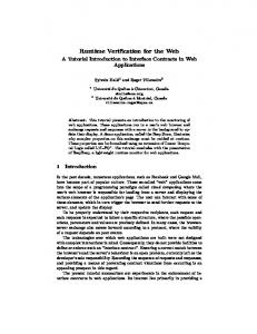
We consider a surveillance system using autonomous aerial drones as a case study to present the challenges in building safe robotics systems and to demonstrate how Drona can be used to address them. Motivating example: Let us consider an application where a drone must patrol a set of locations in a city. Figure 1a shows a snapshot of the workspace from the Gazebo simulator [8]. Figure 1b presents the obstacle map for the workspace with some surveillance points (blue dots) and a possible path that the autonomous drone can take when performing the surveillance task (black trajectory). Obstacles such as houses and cars are considered to be static.

(a) Workspace.

(b) Obstacle map.

Fig. 1: Surveillance system using drones: (a) Workspace created in Gazebo simulator, (b) Obstacle map for the workspace with surveillance points (blue) and an example trajectory of the drone (black).

High level controllers of an autonomous drone performing complex tasks, such as surveillance, usually involve several modes that change during the span

Fig. 2: Operation modes of autonomous drone. of a mission. Figure 2 presents an example of a high level controller and shows how different modes are organized and connected by triggering events. A controller execution can look like: the drone starts in Disarmed state; on receiving the arm command it moves to Armed state where rotors are started; on receiving the takeoff command followed by the autopilot command, the drone moves to the Mission mode where it starts performing the surveillance mission. In each mode, different components cooperate with the goal of performing the desired operations. For instance, in the mission mode components like application, motion planner, and plan executor together ensure that the robot safely performs the surveillance mission. Irrespective of the mode of operation, the high level controller must handle critical events that can happen at any time. For example, a criticalBattery event must be handled correctly by aborting all operations and safely returning to home location. Implementing a high-level controller that satisfies desired properties is notoriously hard. For example, in surveillance applications, the drone should: (P1) Sequencing: Visit all the surveillance points in priority order; (P2) Coverage: Eventually visit all the surveillance points; (P3) Obstacle avoidance: Never collide with an obstacle; (P4) Valid trajectory: Compute valid trajectories leading to the goal location; (P5) Safe trajectories: Follow the reference trajectory within an error bound. These properties involve different reasoning domains and robot components. For instance, properties P1-P2 are application specific and comprise discrete events. Contrarily, properties P3-P5 are generic (i.e., they should be satisfied by any safe robotics system) and concern both discrete and continuous domains. Moreover, properties P3-P4 must be ensured by the motion planner (discrete) that generates trajectories, whereas the property P5 is dependent on the low-level controllers (continuous). These observations motivate the need for decomposing the verification problem into subproblems that can be tackled by using the right technique. For instance, traditional model checking approaches can address properties P1-P2, they could be used to reason on properties P3-P4 under some abstractions/assumption (e.g., state space discretization or robot dynamics linearization), but they hardly provide guarantees about P5 due to the infinite/continuous domains involved. The simulation and testing-based approaches can handle properties P1-P5 but they suffer a lack of guarantees, in the sense that an exhaustive analysis would require an infeasible infinite number of simulations.

Approach Overview: We now give an overview of the new methodology proposed in this paper based on the software stack of a robotics system built using our framework. The software stack is organized into four main blocks (Figure 3): (1) the application block that implements the application specific logic; (2) the trusted software stack that Surveillance System focuses on modules that can be Application reused across different applications; (3) the low-level controllers layer that Motion Planner implements the primitive controllers Online Helper Monitors Modules and state-estimators (possibly proPlan Executor vided by third-parties); (4) the runRV Module Trusted Software Stack time verification block that implements online monitoring to ensure State Controllers that robot always performs safe conEstimators Robot SDK trol actions. The edges in Figure 3 represents interaction between different blocks, for example, the compoFig. 3: Robotics software stack nents in the trusted software stack can create monitors that observe the state of the robot by processing the sensor streams and inform components in trusted software stack if the monitored properties are violated. To reason on the blocks (1) and (2), we use P [6], an event-driven programming language for implementing and model checking high-level logics. A P program comprises state machines communicating asynchronously with each other using events accompanied by typed data values. For blocks (3) and (4) we use Signal Temporal Logic (STL) [7], a formalism suitable to describe properties on real-values signals over real-time. STL is used to define properties related to assumptions needed by the blocks (1) and (2) and to monitor their status at runtime while the drone performs a mission. Our approach can be used to validate properties P1-P4 similar to the traditional verification approaches and simultaneously ensures that the system satisfies property P5 using runtime verification based on STL online monitoring.

3

Terminology and Definitions

In this section, we formalize the definitions needed for the rest of the paper. Workspace: We represent the workspace for a robot W ⊆ R3 as a 3-D occupancy map, where obstacles are assumed to be convex (Figure 1b). The set of all locations occupied by obstacles is denoted by Ω. The set of free locations in the workspace is denoted by F , where F = W \ Ω. Tasks: In an autonomous robotics system, tasks can be generated dynamically and assigned to the robot. An atomic task is represented by the goal location g ∈ F that the robot must visit in order to accomplish the task. A complex task can be represented as a sequence of atomic tasks. For example, moving from one

surveillance point to another is an atomic task and periodically visiting all the surveillance points is an example of a complex task. Trajectory: The motion of a robot operating in W can be expressed by the rule q0 = f (q, u) where q ∈ F is the current robot position, u ∈ Rm is the current input, and q0 ∈ F is the future robot position under the influence of u. We consider the robot as a black-box as we do not explicitly know f , but we can observe the generated trajectories of a robot. A trajectory is a function τ : T → F from a linearly-ordered time domain to a location in the workspace. Let qi , qg ∈ W be two locations and q ∈ F be the current robot position. Let d(q, qg ) be the Euclidean distance between q and qg , and d(q, (qi , qg )) be the distance between q and the line passing through qi and qg . -close: A robot is -close to a location qg represented by close(qg , ) if close(qg , ) := d(q, qg ) < . -tube: A robot is within the -tube surrounding the line passing through points qi and qg , represented by tube((qi , qg ), ), if the distance between its current position and the line is bounded by , i.e., tube((qi , qg ), ) := d(q, (qi , qg )) < . Motion primitives: Motion primitives are a set of short closed-loop trajectories of a robot under the action of a set of precomputed control laws [9,10]. The set of motion primitives form the basis of the motion of a robot. A robot moves from its current location to a destination location by executing a motion plan which is a sequence of motion primitives. The low-level controllers can be used to move the robot from one location to another by continuously changing either its velocity or thrust. We leverage these controllers to implement a motion primitive, called goto, that moves the robot from its current location to the goal location along the straight line joining the locations. Given the complex dynamics of a robot, noisy sensors, and environmental disturbances ensuring that the robot precisely follow a fixed trajectory is extremely hard (see Figure 5). Hence, we assume that on executing goto(qg ), the robot takes any trajectory from its current location qi to the goal location qg such that tube((qi , qg ), ) holds for the duration of the goto, where  is error bound by which the robot can drift. In Section 5, we present formal specification of goto using STL and describe an approach for learning error bound  such that the specification of goto is robust.

4

Trusted Robotics Software Stack

The first part of the proposed framework consists of a generic trusted software stack that implements the common components required for building safe autonomous robots. Our trusted software stack consists of three main components (Figure 3): 1. Motion planner, that computes a safe motion plan from the current position to the goal location required by the current task, 2. Plan executor, that ensures that the robot correctly executes the generated motion plan;

3. Helper modules, consisting of helper state-machines that continuously observe the sensor streams published by the robot sensors and inform the high-level components of important events. Given a high level task, the motion planning problem is to compute a safe motion-plan such that on executing it the robot follows a safe trajectory to its goal location without colliding with any obstacle. The adopted motion planning technique is based on the composition of motion primitives [11]. A motion plan is defined as a sequence of motion primitives that move the robot from its current location to the goal location qg . We use a sampling based approach to compute a motion plan denoted by the sequence µ = (goto(q1 ) . . . goto(qg )), such that, on Fig. 4: Motion plan as a sequence of goto executing µ, the resultant trajectory does not collide with any obstacle and takes the robot to the goal location (see Section 7 for implementation details). Our plan executor ensures that the motion primitives are executed in timely fashion so that the robot follows a safe trajectory. Obstacle collision avoidance is guaranteed by the assumption that the paths taken by the robot lie inside a safe tube (see Figure 4; safe (green) and reference (red) trajectories). The motion planner ensures that the plan tube does not collide with any obstacle. In the following, we will show how such a safe tube can be determined (Section 5) and we will provide a method to monitor whether the drone actually flies inside it (Section 6). Verification approach: To model check our trusted software stack, we implemented each high-level component as a collection of P state machines. The P compiler generates code that can be model checked using state-of-the-art search prioritization techniques (for details, see Section 7). We use over-approximating models for all motion primitives and the robot state during testing, and replace them with their implementations for real execution. In most cases, computing a safe motion plan involves usage of complex constraint solvers [12,11] or graph search (sampling) algorithms [13]. Hence, some part of the motion planner is not implemented in P and is considered as a black-box. When verifying the software stack, creating a sound model of such a motion planner is hard. To resolve this problem, we use execution based model checking [14], a verification technique based on executing the actual program implementation whenever the sound model is not available during the systematic exploration. We extended the model checker such that, whenever the motion planner invokes an external function, it executes its native implementation. This technique is sound because same implementation code is used during model checking and actual execution. To summarize, we provide a method to implement verified motion planners and plan executors (e.g, that satisfy properties like P3-P4). However, the verified

properties hold only under some specific assumptions, for instance, the trajectories taken by the robot are contained by a safe tube (see Figure 4).

5

Validating Low-Level Controllers

When model-checking the high-level software we assumed a discrete abstraction of the motion primitives used to control robot’s motion. For instance, when a goto command is invoked, we assume that the drone reaches the target location in a reasonable amount of time without drifting too much from the nominal line connecting its current position and the target point. In this section, we first specify the motion primitives using parametric Signal Temporal Logic. Next, we use linear regressions to learn the specification parameters for a given robot. Finally, we evaluate these specifications on several observed trajectories. The formalization and analysis of the assumptions about motion primitives allow us to bridge the gap between their discrete abstractions used during model checking and their low-level implementation. 5.1

Signal Temporal Logic

We begin by introducing Signal Temporal Logic [7] (STL), a formalism particularly suitable for the specification of properties of real-values signals over real-time, such as trajectories generated by robots. A signal is a function s : D → S, with D ⊆ R≥0 an interval and either S ⊆ B or S ⊆ R, where B = {>, ⊥} and R is the set of reals. Signals defined on B are called booleans, while those on R are said real-valued. A trace w = {s1 , . . . , sn } is a finite set of real-valued signals defined over the same interval D. Let Σ = {σ1 , . . . , σk } be a finite set of predicates σi : Rn → B, with σi ≡ pi (x1 , . . . , xn ) C 0, C ∈ { UI ϕ, or GI ϕ := ¬FI ¬ϕ. Given a t ∈ R≥0 , a shifted interval I is defined as t+I = {t+t0 | t0 ∈ I}. Definition 1 (Robustness semantics). Let w be a trace, t ∈ R≥0 , and ϕ be an STL formula. The robustness ρ of ϕ for a trace w at time t is defined as: ρ(p(x1 , . . . , xn ) C 0, w, t) = p(w(t)) with C ∈ { 0. The robustness signal of a formula ϕ with respect to w is the signal ρ(ϕ, w, ·). Note that a robot trajectory τ : T → F falls under the definition of trace (see Section 3). With a slight notation overload, we say that a trajectory τ : T → F satisfies a formula ϕ (denoted by τ |= ϕ) if and only if ρ(ϕ, τ, 0) > 0. Differently from classic qualitative semantics, STL robustness provides quantitative information on the evaluated formula, i.e., it tells how strongly the specification is satisfied or violated by the considered trace. In our context, we can use robustness to understand how close a robot trajectory is to a specification violation. For instance, a small positive robustness value means that a slight change in the robot trajectory might lead to a violation. The ability of reasoning on trajectories combined with the qualitative semantics makes STL the right formalism to capture the assumptions that low-level controllers must satisfy.

5.2

Assumptions as STL Formulas

In this section, we use STL to formally specify the goto motion primitive and the motion plan which is a sequence of motion primitives. The assumptions made about the goto motion primitive can be specified as: goto(qg , t, ) := tube((qi , qg ), ) U[0,t] close(qg , )

(3)

This formula holds if the drone stays in the -tube connecting its original position qi and the destination qg until it eventually is -close to the goal point qg . The time interval [0, t] imposes a time constraint on the execution time of the goto command. Recollect that the robot moves from its current location to a goal location by executing a motion plan (a sequence of gotos) generated by the planner (Figure 4). We next specify the set of trajectories that the robot can take when executing a motion plan µ = (goto(qg1 ), . . . , goto(qgn )). Let ξ = (qg1 , . . . , qgn ), t = (t1 , . . . , tn−1 ), and  = (1 , . . . , n−1 ) be sequences of goto locations, the execution times of each goto, and  the parameter corresponding to each goto, respectively. traj(ξ, t, ) is recursively defined as follow: ( traj(ξ, t, ) :=

tube(qg1 , qg2 , 1 ) U[0,t1 ] close(qg2 , 1 )
tube(qg1 , qg2 , 1 ) U[0,t1 ] close(qg2 , 1 ) ∧ traj(ξ 0 , t0 , 0 )

if n = 2 otherwise (4)

where ξ 0 = (qg2 , . . . , qgn ), t0 = (t2 , . . . , tn−1 ), and 0 = (2 , . . . , n−1 ). For the base case, similarly to the goto case, the specification asks the robot to lie in the 1 -tube between qg1 and qg2 until it is 1 -close to the target position qg2 . In the general case, a series of nested until specifications are imposed in order to force the robot to follow the desired sequences of target locations with their corresponding execution times and -tubes.

5.3

Parameter Prediction

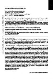
We next describe how we learn the parameter values ( and t) for the goto and traj specifications (Equations 3 and 4) such that they tightly represent the correct sets of behaviors for a given robot. One way to instantiate the specification parameters is to manually choose an upper bound value on the basis of knowledge about the system. However, one value of the parameter might not suffice different templates of the same specification. For instance, consider two goto executions, one to a close location and the other to a distant target location. The duration of the former is likely to be shorter than the latter. A large parameter value for the time duration t satisfies both cases, but for the first one it leads to a highly conservative specification. Similar argument holds for the value of , setting it to a large value means that the radius of -tube is large which makes the motion planner conservative discarding potentially feasible motion plans. In general, we want a mechanism to dynamically tune the parameters depending on the motion primitive. In our case, e.g., goto(qg ) executed at location qi , we want to define two parameter prediction functions ft , f : F × F → R≥0 that return the expected duration t = ft (qi , qg ) and overshoot  = f (qi , qg ) such that the instantiated STL formula goto(qg , t, ) represents the set of valid trajectory specifically for the start location qi and goal location qg . To this end, we adopt regression analysis to estimate  and t as functions of the initial and target locations. We estimate the relationship between the dependent variables  and t and the independent variables l ∈ R≥0 and v ∈ [−1, 1]3 , where l = kqg − qi k and v = (qg − qi )/l are the distance and the normalized direction between qi and qg , respectively. We chose distance and direction as independent variables since we noticed that in our experiments the Fig. 5: goto trajectories evaluation using overshoots () and execution times (t) learned STL specification. are influenced by the direction and distance of the target position. A possible approach to defining prediction functions is to use multilinear regression analysis [15] where the functions are of the form ft (qi , qg ) = xT βt +εt and f (qi , qg ) = xT β + ε where x = (l v) are the independent variables, βt , β ∈ R4 are the parameter vectors, and εt , ε ∈ R are the error terms. Learning parameters: Using multilinear regression, we learned the parameters βt , β , εt , ε analyzing more than 1000 trajectories generated by goto of random lengths. The learned parameters led to the prediction functions: ft (q, qg ) = 30.3438l + 2.3065v1 − 0.9014v2 − 221.1588v3 + 217.6745 f (q, qg ) = 0.1060l − 0.0010v1 − 0.0139v2 + 0.0806v3 + 0.6180

(5)

To demonstrate that the parameters learnt using regressions tightly capture the correct set of behaviors, we present another experiment where the learnt parameter prediction functions are used to automatically instantiate the parameters of STL specifications. Specification instantiation: We analyze the trajectories of the drone repeatedly flying along a tilted eight loop (see Figure 5). From the given way points (stars), we generate the traj STL formula template (Equation 4) and we instantiate it using the prediction functions previously learned (Equation 5). We then evaluate the observed trajectory against the specifications. Figure 5 present 50 trajectories. Green trajectories robustly satisfy the specification (i.e., robustness larger than 0.2); orange ones have a weak positive robustness (i.e., between 0.0 and 0.2); red ones violate the specification (i.e., negative robustness). Note how most of the trajectories satisfy the traj specification and only two violate it, demonstrating that the learnt parameters are tight. This example shows how the proposed parameter prediction method is useful to determined tight parameter evaluations and can be used to validate discrete abstractions used during model checking. However, as these specifications are tight but not sound, it is desirable to have runtime verification for catching outliers.

6

Online Monitoring

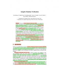
In this section, we provide a method to monitor at runtime the specifications learned in Section 5. An online monitor is useful as it can determine if any of the assumptions (specifications) are violated and notify the operator about the unexpected behavior or trigger some correcting input actions to fix the problem. Differently from the offline approach used in the previous section, online STL algorithms assume that partial traces are provided to the monitor. Partial trajectories might prevent the monitor from computing definitive robustness values. However, online monitors usually provide estimates (upper and lower bounds) of the robustness by quantifying how close is the monitored trace to the violation/satisfaction. To clarify the notion of robustness estimates, consider the formula G[0,10] (x ≥ 0). This specification can be declared satisfied only after observing x on the whole time interval [0, 10]. However, its distance from the violation provides an upper bound of the final robustness. It is important to note that a negative upper bound implies the violation of the specification. There are several methods to Fig. 6: Online goto monitoring using online monitor temporal properlearned STL specification. ties [16,17,18]. In this work, we adopt

the technique presented in [19] where the monitor incrementally computes upper and lower bounds of the robustness by reasoning on the provided partial trace. Intuitively, the online robustness semantics, slightly different from the standard one (Definition 1), provides a best and worst robustness estimates for the partially observed trace. STL online monitoring: We monitor online the traj specification (Equation 4) on one example trajectory. The drone is asked to pass through the way points (stars) that generate a tilted eight loop (see Figure 6). The traj monitor is instantiated with the parameters learnt in Section 5.3. Figure 6 depicts the upper bound robustness signal colored according to its robustness values. Green segments strongly satisfy the specification (i.e., robustness larger than 0.2) while orange ones have a weak positive robustness (i.e., between 0.0 and 0.2). We can observe how the upper bound robustness signal changes from strongly positive (green) to weak positive (orange) along the trajectory. This provides us the exact point at which the trajectory does not strongly (high robustness) satisfy the property, i.e., the instant in which the assumption is getting close to a violation. In our framework, we use the decreasing robustness during online monitoring as a warning to take preemptive action against potential erroneous behavior. To summarize, when a motion plan is executed by a robot in order to accomplish a high-level task, the following sequence of steps are performed: 1. A template of an STL formula is generated corresponding to the motion plan (see Section 5.2); 2. The parameters of the specification are computed using the functions described in Section 5.3; 3. A online monitor is created to monitor the STL specification and take preemptive action based on the robustness value.

7

Implementation and Experimental Evaluation

Our past work on Drona [12] was in the context of distributed mobile robotics. For this work, we reimplemented the framework with runtime verification capabilities and applied to real-world robot systems. In this section, we first describe the implementation of Drona, followed by the empirical evaluation to demonstrate its efficacy for building real-world safe robotics applications. Videos and further details of the conducted experiments are available at https://drona-org.github.io/Drona/. 7.1

Implementation

Figure 7 provides an overview of the Drona framework. The application and the trusted robotics software stack are implemented using the programming language P that allows programmers to write the implementation and its specification at a high-level as a collection of communicating state-machines. P provides firstclass support for modeling concurrency, specifying safety and liveness properties,

and checking that the program satisfies its specification [20,6,21]. We extend P so that programmer can syntactically specify the workspace configuration like obstacle size and its position. The compiler generates code for both executionbased model-checking and real execution when deployed on a target platform. We modified an open-source implementation of the sampling-based motion planner RRT* [13,22] to generate plans as compositions of goto motion primitives. When executing a motion plan, the RV module automatically generates an STL specification (as discussed in Section 5) and performs online monitoring to catch violations. We use Matlab toolbox Breach [23] to online monitor the STL specifications. For our experiments, we use 3DR Iris [24] drone that comes with the open-source Pixhawk PX4 [25] autopilot. We implemented a collection of motion primitives using the low-level controllers provided by the PX4 firmware that is used to control the drone in autopilot mode. Implementation in P

Autogenerated C Code

Application DRONA Compiler

Autogenerated C Code DRONA Runtime

(Trusted)

Online Monitors for RV

Robot Firmware Reproducible Error Trace

DRONA Systematic Testing Tool

(low level controllers and estimators)

Robot Hardware Or Simulator

Fig. 7: Overview of Drona tool chain

7.2

Deployed System

Generic Robotics Software Modules

Some examples of the implemented motion primitives are arm, takeoff, goto. When invoked, motion primitives are converted into series of MAVLINK messages (a protocol for communicating with unmanned vehicles) and sent to drone via User Datagram Protocol (UDP).

Evaluation

As a case study, we implemented a safe real-world surveillance application. Safe surveillance: The entire surveillance system, which includes application and the trusted software stack, was implemented in around 3500 lines of P code and was systematically tested using the execution-based model-checker. We found some critical bugs in our high-level software implementation. For example, we did not check that when the battery is low the drone should not take-off. This bug was uncovered by the model checker within a few minutes but was not found during simulations as the simulator always starts in full battery state. After model-checking, we also performed stress-testing by running the surveillance application for several hours performing software-in-the-loop simulation. We did not find any new bugs in our implementation, except for some bugs at the interface of the P and external C code. This example demonstrates that model checking performs better than simulation-based testing in providing testcoverage and finding bugs in robotics software. Obstacle avoidance: We next present simulation results to demonstrate the effectiveness of our STL-based online monitoring approach. We created a surveillance workspace in Gazebo [8] simulator environment (Figure 1a) that is internally represented by Drona as an obstacle map (Figure 1b). In our simulations,

we execute the PX4 firmware in the loop, meaning that we considered a real lowlevel controller implementation that can be executed in the real deployment. We consider an obstacle avoidance scenario, where the drone must never get closer than 0.5m to any obstacle in the workspace during its 120s of flight. The corresponding STL formula is: ϕobs :=

n ^

¬F[0,120] (d(q, obsj ) < 0.5)

(6)

j=1

where q ∈ F is the robot current position, and d(q, objj ) represents the distance between robot current position and the j-th obstacle. We online monitored the requirement ϕobs on all the trajectories generated by the drone during the surveillance task. Figure 8 shows two views of a faulty trajectory of the drone with the upper bound of its online robustness. Note how online monitoring detects a specification violation (red trace), meaning that the drone gets too close (< 0.5m) to an obstacle. Also, observe that the robot robustly satisfy the specification in most part of the trajectory, with the exception of few segments where the robustness is between 0 and 0.5 (orange traces).

Fig. 8: Online obstacle avoidance monitoring (Equation 6). Robustness legend: green [0.5, +∞), orange (0, 0.5), red [−∞, 0). Plan execution: In this case, we monitor the correctness of the trajectories taken by the drone with respect to the reference ones computed by the motion planner. Recollect that given a task, the motion planner returns a sequence of waypoints or locations whose linear interpolation takes the drone from its current position to the goal location. For every such path, we are interested in checking whether the drone reaches all the waypoints while remaining inside a safe -tube. To this end, we generated the STL specification in Equation 4 on the fly using the locations returned by the motion plan and instantiated its parameters using the prediction functions learned in Section 5.3. Note that Drona builds an STL specification for every generated plan. Once that the specification is generated, the online monitoring module checks it against the actual trajectory. Figure 9 shows the robustness upper bound for an example trajectory computed online. It is interesting to note how there are two falsifying segments (red),

i.e., parts of the trajectory that do not satisfy the generated STL specifications. Note how both these segments refer to parts where the drone strays away from the reference trajectories (dashed). The graph also shows some nonrobust traces (orange) where the drone is quite distant from the reference trajectories but does not violate the generated specification. Finally, note how in most part of the trajectory the robustness is green as it is always close to the reference.

Fig. 9: Online trajectory following (Equation 4 with predicted parameters of Equation 5). Robustness legend: green [0.2, +∞); orange (0, 0.2); red [−∞, 0).

8

Related Work

Recently, there is increased interest towards using temporal logic formalism for synthesizing reactive robotics software [26,27,28,29,30,31]. This approach provides strong guarantees of correctness. However, the problem with automated synthesis is that the algorithms scale poorly both with the complexity of the mission and the size of the workspace. Reachability analysis techniques have been used to verify robots modeled as hybrid systems. Some examples of numeric analyzers are SpaceEx [32], Flow∗ [33], Sapo [34], or C2E2 [40]. Symbolic analyzers are also available, such as KeYmaera [35], dReach [36], or pyHybridAnalysis [37]. Differently from this work, reachability methods require an explicit representation of the robot dynamics and often suffer from scalability issues. Simulationbased tools for the falsification of black-box systems (such as Simulink or Stateflow models) are more scalable than reachability methods but generally, they do not provide any formal guarantees. In this case, the goal of the falsifier is to generate a model simulation that does not satisfy a given specification. Some STL and MITL falsification tools are Breach [23], S-TaLiRo [38], or RRT-Rex [39]. Finally, the idea of synthesizing monitors from specifications [41,42,43] is well studied in the runtime verification community. Runtime verification has been applied to robotics [44,45,46,47] where monitors are used to checking the status of path planner and tasks executions. The related work for this paper addresses different parts of the robotics software stack, our approach combines these wellknown approaches in a practical way to build real-world robotics applications.

References 1. A. Marino, L. Parker, G. Antonelli, and F. Caccavale, “Behavioral control for multi-robot perimeter patrol: A finite state automata approach,” in International Conference on Robotics and Automation, ICRA, pp. 831–836, IEEE, 2009. 2. A. Barrientos, J. Colorado, J. d. Cerro, A. Martinez, C. Rossi, D. Sanz, and J. Valente, “Aerial remote sensing in agriculture: A practical approach to area coverage and path planning for fleets of mini aerial robots,” Journal of Field Robotics, vol. 28, no. 5, pp. 667–689, 2011. 3. B. Kehoe, S. Patil, P. Abbeel, and K. Goldberg, “A survey of research on cloud robotics and automation,” IEEE Transactions on Automation Science and Engineering, vol. 12, no. 2, pp. 398–409, 2015. 4. V. K. Omachonu and N. G. Einspruch, “Innovation in healthcare delivery systems: a conceptual framework,” The Public Sector Innovation Journal, vol. 15, no. 1, pp. 1–20, 2010. 5. T. Yamaguchi, T. Kaga, A. Donz´e, and S. A. Seshia, “Combining requirement mining, software model checking, and simulation-based verification for industrial automotive systems,” in Proceedings of the IEEE International Conference on Formal Methods in Computer-Aided Design (FMCAD), October 2016. 6. A. Desai, V. Gupta, E. Jackson, S. Qadeer, S. Rajamani, and D. Zufferey, “P: Safe asynchronous event-driven programming,” in Programming Language Design and Implementation (PLDI), pp. 321–332, 2013. 7. O. Maler and D. Nickovic, “Monitoring temporal properties of continuous signals,” in Formal Techniques, Modelling and Analysis of Timed and Fault-Tolerant Systems, pp. 152–166, Springer, 2004. 8. N. Koenig and A. Howard, “Design and use paradigms for gazebo, an open-source multi-robot simulator,” in Intelligent Robots and Systems, IROS. 9. S. M. LaValle, Planning algorithms. Cambridge university press, 2006. 10. D. Mellinger and V. Kumar, “Minimum snap trajectory generation and control for quadrotors,” in International Conference on Robotics and Automation (ICRA), pp. 2520–2525, 2011. 11. I. Saha, R. Ramaithitima, V. Kumar, G. J. Pappas, and S. A. Seshia, “Automated composition of motion primitives for multi-robot systems from safe ltl specifications,” in Intelligent Robots and Systems, IROS, pp. 1525–1532, IEEE, 2014. 12. A. Desai, I. Saha, J. Yang, S. Qadeer, and S. A. Seshia, “Drona: A framework for safe distributed mobile robotics,” in Proceedings of the 8th International Conference on Cyber-Physical Systems, ICCPS ’17, (New York, NY, USA), pp. 239–248, ACM, 2017. 13. S. Karaman and E. Frazzoli, “Incremental sampling-based algorithms for optimal motion planning,” Robotics Science and Systems VI, vol. 104, 2010. 14. P. Godefroid, “Model checking for programming languages using verisoft,” in Proceedings of the 24th ACM SIGPLAN-SIGACT symposium on Principles of programming languages, pp. 174–186, ACM, 1997. 15. J. Neter, M. H. Kutner, C. J. Nachtsheim, and W. Wasserman, Applied linear statistical models, vol. 4. Irwin Chicago, 1996. 16. O. Maler and D. Niˇckovi´c, “Monitoring properties of analog and mixed-signal circuits,” International Journal on Software Tools for Technology Transfer, vol. 15, no. 3, pp. 247–268, 2013. 17. H.-M. Ho, J. Ouaknine, and J. Worrell, “Online monitoring of metric temporal logic,” in Runtime Verification, RV, pp. 178–192, Springer, 2014.

18. A. Dokhanchi, B. Hoxha, and G. E. Fainekos, “On-line monitoring for temporal logic robustness.,” in Runtime Verification, RV, pp. 231–246, 2014. 19. J. V. Deshmukh, A. Donz´e, S. Ghosh, X. Jin, G. Juniwal, and S. A. Seshia, “Robust online monitoring of signal temporal logic,” in Runtime Verification, RV, pp. 55– 70, Springer, 2015. 20. “P Github.” https://github.com/p-org/P, 2017. 21. A. Desai, S. Qadeer, and S. A. Seshia, “Systematic testing of asynchronous reactive systems,” in Foundations of Software Engineering (FSE), pp. 73–83, 2015. 22. I. A. S ¸ ucan, M. Moll, and L. E. Kavraki, “The Open Motion Planning Library,” IEEE Robotics & Automation Magazine, vol. 19, pp. 72–82, December 2012. http: //ompl.kavrakilab.org. 23. A. Donz´e, “Breach, a toolbox for verification and parameter synthesis of hybrid systems,” in Computer Aided Verification, CAV, pp. 167–170, 2010. 24. “3D Robotics.” https://3dr.com/, 2017. 25. “PX4 Autopilot.” https://pixhawk.org/, 2017. 26. O. Kupferman and M. Y. Vardi, “Model checking of safety properties,” Formal Methods in System Design, vol. 19, no. 3, pp. 291–314, 2001. 27. H. Kress-Gazit, G. E. Fainekos, and G. J. Pappas, “Temporal-logic-based reactive mission and motion planning,” IEEE transactions on robotics, vol. 25, no. 6, pp. 1370–1381, 2009. 28. I. Saha, R. Ramaithitima, V. Kumar, G. J. Pappas, and S. A. Seshia, “Implan: scalable incremental motion planning for multi-robot systems,” in International Conference on Cyber-Physical Systems (ICCPS), pp. 1–10, IEEE, 2016. 29. G. E. Fainekos, H. Kress-Gazit, and G. J. Pappas, “Temporal logic motion planning for mobile robots,” in International Conference on Robotics and Automation, ICRA, pp. 2020–2025, IEEE, 2005. 30. G. E. Fainekos, A. Girard, H. Kress-Gazit, and G. J. Pappas, “Temporal logic motion planning for dynamic robots,” Automatica, vol. 45, no. 2, pp. 343–352, 2009. 31. I. Saha, R. Ramaithitima, V. Kumar, G. J. Pappas, and S. A. Seshia, “Automated composition of motion primitives for multi-robot systems from safe ltl specifications,” in International Conference on Intelligent Robots and Systems (IROS), pp. 1525–1532, IEEE, 2014. 32. G. Frehse, C. Le Guernic, A. Donz´e, S. Cotton, R. Ray, O. Lebeltel, R. Ripado, A. Girard, T. Dang, and O. Maler, “Spaceex: Scalable verification of hybrid systems,” in Computer Aided Verification, CAV, pp. 379–395, Springer, 2011. ´ 33. X. Chen, E. Abrah´ am, and S. Sankaranarayanan, “Flow*: An analyzer for nonlinear hybrid systems,” in Computer Aided Verification, CAV, pp. 258–263, 2013. 34. T. Dreossi, “Sapo: Reachability computation and parameter synthesis of polynomial dynamical systems,” in Hybrid Systems: Computation and Control, HSCC, HSCC ’17, pp. 29–34, 2017. 35. A. Platzer and J. Quesel, “Keymaera: A hybrid theorem prover for hybrid systems (system description),” in International Joint Conference on Automated Reasoning, IJCAR, pp. 171–178, 2008. 36. S. Kong, S. Gao, W. Chen, and E. Clarke, “dreach: δ-reachability analysis for hybrid systems,” in Tools and Algorithms for the Construction and Analysis of Systems, TACAS, pp. 200–205, Springer, 2015. 37. A. Casagrande and T. Dreossi, “pyhybrid analysis: A package for semantics analysis of hybrid systems,” in Euromicro Conference on Digital System Design, DSD, pp. 815–818, 2013.

38. Y. Annpureddy, C. Liu, G. E. Fainekos, and S. Sankaranarayanan, “S-taliro: A tool for temporal logic falsification for hybrid systems,” in Tools and Algorithms for the Construction and Analysis of Systems, TACAS, pp. 254–257, 2011. 39. T. Dreossi, T. Dang, A. Donz´e, J. Kapinski, X. Jin, and J. Deshmukh, “Efficient guiding strategies for testing of temporal properties of hybrid systems,” in NASA Formal Methods, NFM, pp. 127–142, 2015. 40. P. S. Duggirala, S. Mitra, M. Viswanathan, and M. Potok, “C2E2: a verification tool for stateflow models,” in International Conference on Tools and Algorithms for the Construction and Analysis of Systems, pp. 68–82, Springer, 2015. 41. K. Havelund and G. Ro¸su, “Synthesizing monitors for safety properties,” in Tools and Algorithms for the Construction and Analysis of Systems, TACAS, pp. 342– 356, Springer, 2002. 42. S. D. Stoller, E. Bartocci, J. Seyster, R. Grosu, K. Havelund, S. A. Smolka, and E. Zadok, “Runtime verification with state estimation,” in International Conference on Runtime Verification, pp. 193–207, Springer, 2011. 43. E. Bartocci, R. Grosu, A. Karmarkar, S. A. Smolka, S. D. Stoller, E. Zadok, and J. Seyster, “Adaptive runtime verification,” in Runtime Verification, RV, pp. 168– 182, Springer, 2012. 44. E. Gat, M. G. Slack, D. P. Miller, and R. J. Firby, “Path planning and execution monitoring for a planetary rover,” in Robotics and Automation, pp. 20–25, IEEE, 1990. 45. O. Pettersson, “Execution monitoring in robotics: A survey,” Robotics and Autonomous Systems, vol. 53, no. 2, pp. 73–88, 2005. 46. A. Lotz, A. Steck, and C. Schlegel, “Runtime monitoring of robotics software components: Increasing robustness of service robotic systems,” in Advanced Robotics (ICAR), 2011 15th International Conference on, pp. 285–290, IEEE, 2011. 47. I. Lee, H. Ben-Abdallah, S. Kannan, M. Kim, O. Sokolsky, and M. Viswanathan, “A monitoring and checking framework for run-time correctness assurance,” 1998.