real-world formulation of the course timetabling problem to test prac- ..... Table 1: Algorithm parameters for the two benchmark problems. Parameter. Onemax .... Normality and Homocesticity of the data was checked using Shapiro-wilk test.
Combining Mutation and Recombination to Improve a Distributed Model of Adaptive Operator Selection Jorge A. Soria-Alcaraz 1 , Gabriela Ochoa 2 , Adrien G¨ oeffon3 , Fr´ed´eric Lardeux3 , Fr´ed´eric Saubion3 1
Universidad de Guanajuato - Divisi´ on de Ciencias Econ´ omico-Administrativas Depto de Estudios Organizacionales, 2 University of Stirling, 3 University of Angers
Abstract. We present evidence indicating that adding a crossover island greatly improves the performance of a Dynamic Island Model for Adaptive Operator Selection. Two combinatorial optimisation problems are considered: the Onemax benchmark, to prove the concept; and a real-world formulation of the course timetabling problem to test practical relevance. Crossover is added to the recently proposed dynamic island adaptive model for operator selection which considered mutation only. When comparing the models with and without a recombination, we found that having a crossover island significantly improves the performance. Our experiments also provide compelling evidence of the dynamic role of crossover during search: it is a useful operator across the whole search process. The idea of combining different type of operators in a distributed adaptive search model is worth further investigation.
1
Introduction
Search operators are key elements of heuristic search algorithms, determining the structure of the fitness landscape being searched. A large variety of operators have been proposed in the literature for combinatorial optimisation problems. However, given a new problem or instance of a combinatorial problem it is not clear before hand which operator (or indeed set of operators) will be the most effective. In response to this, modern heuristic approaches combine several operators. Some schemes such as variable neighbourhood search, or standard memetic algorithms combine operators in a pre-determined way. Some other schemes, such as hyper-heuristics [2, 12], and adaptive operator selection approaches [10], acknowledge the advantage of combining a pool of operators; but most importantly, they also realise that the usefulness of specific operators can vary dynamically across the search process. Therefore, they propose adaptive, learning-based mechanisms for selecting operators on the fly. Island models [18] were initially introduced for avoiding premature convergence in evolutionary algorithms (EAs). They use a set of sub-populations instead of a single a panmictic one. Sub-populations evolve independently on separated islands during some search steps and interact periodically with other
islands by means of migrations [14], whose impact has been carefully studied [8, 9]. Two main types of island models can be considered. First, replicating the same algorithm on each island with the view of improving the management of the population. This constitutes the most common use of island models and is closely related to distributed evolutionary algorithms [9]. Second, considering different algorithms (or algorithms settings) on each island as a dynamic control method in order to identify the most promising algorithm according to the current state of the search. Island models traditionally use fixed migration policies in order to reinforce the islands characteristics [15, 6, 1]. An alternative dynamic migration policy was proposed by Lardeux and Go¨effon [7], where migration probabilities change during the evolutionary process according to the impact of previous analogue migrations. The island model should be able to both identify the current most appropriate subset of islands for improving individuals, and to quickly react to changes if other heuristics (operators) turn out to be more beneficial. It is important to stress that in this article, the island model does not implement a complete evolutionary algorithm in each island as it is usually done. Instead, each island is associated with a single (different) search operator, and in every iteration the island’s operator is applied to all individuals in the island. This constitutes an approach to adaptive operator selection as recently proposed by Candan et al.[3]. The ability of the dynamic island model to efficiently manage simple operators has already been compared to other adaptive operator selection approaches in [3] . So far, mutation operators or abstract scenarios have been considered. The motivation of this paper is to assess the efficiency of the island model in presence of different kinds of operators, such as crossover on various problems. The idea is to assign an operator to each island and use the dynamic regulation of migrations to distribute the individuals on the most promising islands (i.e., the most efficient operators) at each stage of the search. The main contribution of this article is the introduction of crossover in conjunction with mutation operators, while the original adaptive operator selection model considered only mutation operators [3]. In our proposal, individuals from different islands can undergo recombination when they “visit” the recombination island and thus may directly share information. We found that having a crossover island significantly improves the model’s performance. We demonstrate this by comparing the models with and without recombination on two selected benchmarks: the Onemax problem, widely used to prove concepts in adaptive operator selection studies [5, 4, 3]; and a formulation of the course timetabling problem considering the set of publicly available real-world instances from the 2007 International Timetabling Competition ITC-2007 [11]. The article is organised as follows. Section 2 introduces the dynamic island model of adaptive operator selection, and how we incorporated crossover into it. Section 3 describes the experimental setting, while results are presented in Section 4. Finally, Section 5 summarises our findings and suggests directions for future work.
2
Crossover as an Island Operator
We start by formally presenting the dynamic island model for adaptive operator selection and follow by describing how crossover was incorporated.
2.1
Dynamic Island Model
Let us consider an optimisation (minimisation) problem defined as a pair (S, f ) where S is a search space whose elements represent candidate solutions of the problem, and f : S → R is an objective function. An optimal solution is an element s∗ ∈ S such that ∀s ∈ S, f (s∗ ) > f (s). An Island Model can be formally defined as a tuple (I, H, P, V, M ). Where I = {i1 , · · · , in } is the set of Islands, H = {H1 , · · · , Hn }, a set of heuristics (operators in this paper), and P = {p1 , · · · , pn } a collection of sub-populations, one per island. The topology of the model is given by an undirected graph G(I, V ) where V ⊆ I 2 is a set of edges between islands (I, the nodes of the graph.) Finally, the migration policy is given by a square matrix M of size n, such that M (i, j) ∈ [0, 1] represents the probability for an individual to migrate from island i to island j. Each island k is equipped with a sub-population pk and an operator Hk . The matrix M is coherent with the topology, i.e., if (i, j) 6∈ V then M (i, j) = 0. Algorithm 1 outlines the operation of an Island Model for minimisation problems.
Algorithm 1 Basic Island Model Require: an IM (I, A, P, V, M ), an Optimisation problem (S, f ) 1: while not stop condition do 2: for i ← 1 to n do 3: pi ← Hi (pi ) 4: for s ∈ pi do 5: for j ← 1 to n do 6: generate a random number rand 7: if rand < M (i, j) and |pi | > 0 then 8: pj ← pj ∪ {s} 9: pi ← pi \ {s} 10: end if 11: end for 12: end for 13: end for S 14: b ← best( i (pi )) 15: if f (b) > f (s∗ ) then 16: s∗ ← b 17: end if 18: end while 19: return s∗
In the algorithm, pi denotes the sub-population at island i and Hi (pi ) (line 3) the population obtained after applying heuristics Hi on it. The function best computes the best current individual w.r.t. objective function f . The stopping condition is, as usual, a limited number of iterations or the fact that an optimal solution has been found in the global population. The migration matrix M is used to send individuals to other islands or stay on the same one. In dynamic island models, an adaptive update of the migration matrix at iteration t + 1, denoted Mt+1 , is performed as: Mt+1 (i, k) = (1 − β)(α.Mt (i, k) + (1 − α)Ri,t (k)) + βNt (k) where Nt is a stochastic noise vector such that ||Nt || = 1 and Ri,t is a reward vector that is computed after applying Hi at time t. α allows to control the balance between previous knowledge accumulated and immediate observed effect. β controls the amount of noise, which is necessary to explore alternative actions. These parameters need to be tuned and their impact has been studied in [3]. The reward Ri,t (k) is defined as: ( Ri,t (k) =
1 |B|
if k ∈ B,
0
otherwise,
where B is the set of the operators that have been produce the best improvement for each island i.e., operators producing the best improvements according tof for each island at a given time. 2.2
Incorporating Crossover
Mutation heuristics perform a change on a given solution, by swapping, changing, removing, adding or deleting solution components. In contrast crossover operators, take two (or more solutions), combine them and return a new solution (or more than one solution). Let s ∈ S be a solution. A (unary) mutation operator can be formally defined as Hm : S → S. Crossover operators can in turn, be defined with the following signature Hc : S × S → S × S. We propose to incorporate crossover as an island operator. The key idea is to define the crossover Hc with a similar formal signature than mutation Hm .
Algorithm 2 Standard Operator Island Require: a population p 1: OffspringPool = ∅ 2: for all s ∈ p do 3: OffspringPool = OffspringPool ∪ {H(s)} 4: end for 5: return OffspringPool
Algorithm 2 outlines the behaviour of an operator island in the island model. The operator H is applied at line 3. The crossover island uses the same overall Algorithm 2, but to apply recombination (Hc ) with the same signature than mutation, it requires a single solution as parameter. The crossover is performed using the incoming solution as one parent. The other parent is either a random solution (only for the first iteration) or the last incoming solution. The best generated offspring is then returned. This is outlined in Algorithm 3. With this simple mechanism we can combine mutation and recombination operators in the island model for adaptive operator selection.
Algorithm 3 Crossover Operator Hc Require: s incoming solution 1: if T emp is undefined then 2: T emp = randomSolution() 3: end if 4: Of f springs = Crossover(T emp, s) 5: T emp = s 6: return Best(Of f springs)
3
Experimental Setup
Two algorithm variants are considered: DIM-M, a dynamic island model of adaptive operator selection with mutation operators only, and DIM-MX, which combines mutation and recombination. They are tested using the benchmark problems and algorithm setting described below. Onemax: (or counting ones problem), is a unimodal maximisation problem traditionally used in theoretical and proof of concept studies in genetic algorithms, where the string of all ones is the single optimum. Following Candan et.al [3] we use a Onemax instance of size n = 1000, the algorithm parameters are summarized in Table 1. Four mutation operators and one recombination operator are considered. Each operator is assigned to an island and it is applied regardless of whether it improves or not the incoming solution. The operators used are: – bit-flip mutation: flips each bit with probability 1/n. – k-bit mutation: (with k= 1, 3, 5), chooses uniformly at random k bits in the current solution and flips their values. – 1-point crossover : chooses uniformly at random position in the string, and interchanges the sub-strings to produce offspring. Course Timetabling: is a minimisation problem where the objective is to assign several events to time-slots without violating certain constraints. The problem can be defined in terms of a set of events (courses or subjects) E = {e1 , e2 , . . . , en }, a set of time-periods T = {t1 , t2 , . . . , ts }, a set of places (classrooms) P = {p1 , p2 , . . . , pm }, and a set of agents (students registered in the
courses) A = {a1 , a2 , . . . , aq }. An assignment is then given by the quadruple (e ∈ E, t ∈ T, p ∈ P, a ∈ A), and a solution to the problem is a complete set of n assignments (one for each event) that satisfies the set of hard constraints. Our formulation uses a generic modelling approach where solutions are encoded as vectors of integer numbers of length equal to the number of events (courses) [16, 17]. Positions in the vector represent events, and their integer values are indices in a set of data structures encoding pairs of valid time-slots and classrooms for each event [16]. A set of four mutation operators are considered, which were the best performing in [17]. They range from simple randomised exchange or swap neighbourhoods to greedy and more informed procedures. As a crossover operator we implemented the simple 1-point crossover. This is possible with the representation used (a vector if integer numbers) where offspring generated by 1-point crossover are valid solutions. – Simple Random Perturbation (SRP): uniformly at random chooses a variable and changes its value for another one inside its feasible domain. – Swap (SWP): selects two variables uniformly at random and interchanges their values. – Statistical Dynamic Perturbation (SDP): chooses a variable following a probability distribution based on the frequency of variable selection in the last k iterations. Variables with lower frequency will have a higher probability of being selected. Once selected, the value is randomly changed. – Double Dynamic Perturbation (DDP): similar in operation to SDP, but internally maintains an additional solution, and returns the best of the two solutions. – 1-point crossover : chooses uniformly at random position in the vector, and interchanges the sub-portions to produce offspring. The experiments considered the 24 real-world instances from the 2007 International Timetabling Competition ITC-2007, track 2, which correspond to the post-enrollment course timetabling benchmark1 . These instances range from 400 to 600 events. Table 1 reports the algorithm parameters used. Experiments were conducted on a CPU with Intel i7, 8GB Ram using the Java language and the 64 bits JVM.
4
Results
4.1
Onemax
Figure 1 illustrates an example run of the two algorithm variants on the Onemax problem. DIM-M contains 4 islands, one for each mutation operator, while DIMMX has 5 islands, corresponding to the 4 mutations and the 1-point crossover. 1
Available at http://www.cs.qub.ac.uk/itc2007/
Table 1: Algorithm parameters for the two benchmark problems. Parameter Onemax Course Timetabling Chromosome length 1000 400 to 600 Population size 800 1000 Number of islands 4 or 5 (one for each operator) Initial migration 1/ number-of-islands (α, β) (0.8,0.1) (0.8,0.1) No. of runs 10 10 per instance Stop Criteria Optimum is found 540 sec
The curves show, for each operator (island), the sub-population size over time measured as iterations, and reported at intervals of length 150 (the X values are ×10). We consider an iteration as a single complete execution of the DIM algorithm, which this corresponds to a move or migration of individuals across islands. The plot also shows (the black solid line) the best individual fitness over time, with values visible in the right-hand axis. The variant without crossover (DIM-M, left plot) required over two minutes (128.32 seconds) to reach the global optimum, which corresponds to nearly 7,000 iterations and 68,251 functions calls. The plot shows how the most explorative 5-bit operator has the highest attraction rate at the very early stages of the search. Soon, after 50 iterations or so, this rate goes down leaving a less perturbative operator (namely, 1-bit) to take the lead in the search process. The variant with recombination (DIM-MX, right plot) reached the optimum much faster, in less than 30 seconds, which corresponds to 1,300 iterations and 17,363 functions calls. The plot illustrates the run up to 7,000 iterations for comparisons purposes with the DIM-MX variant. In this case, the crossover operator attraction rate increases steadily up to the point where the optima solution is found. Another interesting observation from these experiments is the superiority of the 1-bit mutation over the more standard bit-flip operator for this problem. Figure 2 offers a close up of the first 3,000 iterations showing population size at each step and considering only two operators for each variant: 1-bit and 5-bit for DIM-M and, 1-bit and crossover for DIM-MX. Note that the horizontal axis shows multiples of 10 iterations. As the right plot of Fig. 2 illustrates, crossover is increasingly useful for DIM-MX search up to the point where the optimal solution is found, which occurs around iteration 1,300. This confirms an interesting property of crossover, which was observed by Ochoa et al. before [13]. Crossover is a versatile operator, its role is dynamic: when there is high diversity in the population such as at the beginning of the search process, it acts as an explorative operator. However, when the population diversity is low (i.e., the population is largely converged) it acts instead an improvement operator preserving the useful building blocks. For Onemax, it is clear that, at the beginning of the search when individuals have low quality (i.e., contain few ones) and are very different, crossover may quickly generate new individuals with more ones by recombination and thus quickly explore more interesting areas. While
legend bit−flip
1−bit
5−bit
3−bit
Croosover
DIM-M
Fitness
DIM-MX 1000
1000
Population Size
Population Size
500
Fitness
Fitness
500
750
200
750
200
100
100
250
250
0
0 0
150
300 Iterations 450
600
0
150
300 Iterations 450
600
Fig. 1: Onemax. Attraction rate (sub-population size) of each operator (island) along with best fitness over time. Values in the X axis multiplied by 10 give iterations. DIM-M, using mutation operators only. DIM-MX, combining mutation with a crossover operator.
when the population has converged to higher quality (i.e., when individuals contains mainly ones), crossover may also be useful by preserving the components of the highly fit individuals. The probability of selecting crossover eventually drops after the optimal solution is found (iteration 1,300) and the performance curve flattens. This is probably due to the computational overhead of crossover as compared to mutation operators. So, it ceases to be selected when no additional improvements are found in the search process. But clearly the operator was increasingly useful from the early stages of the search up to the point when the optimal solution was found. Therefore, crossover is a useful operator across all the search process.. This contrasts with the behaviour of 5-bit on the left plot of Fig. 2 (DIM-M), where 5-bit acts an efficient explorative operator early on (up to iteration 500 or so), but then it stops being useful, as it becomes too disruptive and its rate drops (which has also been observed in [3]). 4.2
Course Timetabling
As a first experiment, we ran the two algorithm variants for two minutes (120 seconds) on a selected course timetabling instance. Specifically, instance number 1 from the ITC-2007 track 2 set, which consists of 500 students, 400 courses, 35 time-slots and 10 classrooms. Again, DIM-M contains 4 islands, one for each mutation operator, while DIM-MX has 5 islands, corresponding to the 4 mutations and the 1-point crossover. Figure 3 illustrates the results. The curves show, for each operator, the sub-population size over time (measured as iterations, at
DIM-M
DIM-MX 1000
1000
variable 1−bit
variable 1−bit
5-bit
Croosover
Fitness
750
100
Population Size
500
Fitness
500
Fitness
750
200
Fitness
Population Size
200
100 250
250
0 0
75
150 Iterations 225
300
0 0
75
150 Iterations 225
300
Fig. 2: Onemax. Close up of the attraction rate (sub-population size) of each operator (island) along with best fitness over time, for the first 3,000 iterations. Values in the X axis multiplied by 10 give iterations. DIM-M, illustrating 1-bit and 5-bit . DIM-MX, illustrating 1-bit and crossover
intervals of length 250). The black solid line in the plots shows the best individual fitness over time, with values indicated in the right-hand axis. In this case, we are dealing with a minimisation problem. It can be seen that the number of iterations is 9250 for DIM-M (left plot), while it is of 6800 iterations for DIMMX. This is because an DIM-MX iteration uses more resources as it consists of 5 operators. Despite this increased CPU demand, the variant with crossover produces the best results at the end of the 120 seconds run. Specifically, DIM-MX finds a solution with fitness 582 (as seen in the right axis with fitness values), which is a much better value (we’re mimimising soft-constraints violations) than the 845 solution achieved by DIM-M. The dynamic rates of the operators across the run is more complex for this problem than for the Onemax (Figs. 1 and 2). The operators combine efforts and take turns in solving the problem. The curves, however, indicate that when recombination is not used (DIM-M, left plot), the swap (SWP) operator dominates the search, specially at the initial and middle stages, while for the DIM-MX variant (right plot), crossover dominates at several stages and enhances the search process. For a more thorough comparison, we used the experimental conditions and rules followed in the timetabling competition. Specifically, we used the benchmark program provided in the competition site to measure the allowed running time on a given machine. This time is generally between 300 and 600 seconds (per run, per instance) on a modern PC. Following the competition protocol, 10 replicas per instance were considered, and the remaining algorithm parameters are reported in Table 1. Table 2 shows results over some representative instances. The variant with recombination DIM-MX, consistently produced the best results across all the instances. Moreover, results with DIM-MX show a much lower standard deviation. We suggest that this occurs because crossover guides the search by combining
legend SRP
SDP
DDP
SWP
Croosover
Fitness
DIM-M
DIM-MX 2000
2000
200
1620
1250
100
100
875
875
500
500 0
150
300
Iterations
600
750
900
0
75
150
225
300 Iterations 450
525
600
675
Fig. 3: Course Timetabling, instance ITC-2007-1. Attraction (sub-population size) of each operator (island) along with best fitness over time. Values in the X axis multiplied by 10 give iterations. DIM-M, using mutation operators only. DIM-MX, combining mutation with a crossover operator.
information from the whole population, and contributes to escape local optima. For the mutation-only variant, migration among islands is the only mechanism for information exchange. It is more likely in this case for an island to be trapped in a local optima.
Table 2: Course Timetabling. Representative ITC-2007 instances. Results are ¯σ shown in the form of: X Instance No. 1 4 10 15 18 20 23 DIM-M 345.2245.23 690.5662.49 2778.2210.4 30.412.1 40.1532.84 186.1438.12 1677.14420.2 DIM-MX 131.1640.10 586.3137.78 2358.2165.3 7.75.3 22.1622.30 150.1015.2 1378.4290.3
A statistical analysis of the results across all test instances was also conducted. Normality and Homocesticity of the data was checked using Shapiro-wilk test. The results of a two-way ANOVA test combining the 24 test instances and 2 algorithm variants is reported in Table 3. The test indicates whether (or not) the means of several groups are equal, which in this context refers to whether the competing algorithms have the same performance across the tests instances. The obtained results support the existence of significant performance differences between the DIM variants. The numbers in bold font under the (P r(> F )) label in Table 3 show the corrected p-value. This value represents the probability of obtaining a test statis-
Fitness
1250
Fitness
Population Size
1620
Population4Size
200
tic result at least as extreme or as close to the one that was actually observed, assuming that the null hypothesis is true (H0 : algorithms have the same performance). Further analysis is provided to identify by other statistical test if the pair of algorithms have significantly different performance. This is achieved with Tukey HSD test with confidence level of 95% (reported at the bottom of Table 3), again the corrected p-value (0.0) give us a very strong presumption against null hypothesis.
Table 3: Course Timetabling. Two-way ANOVA F test, pairwise t test and Tukey HSD test. ANOVA Df Sum Sq Mean Sq Algorithm 1 736576 736576 Instance 23 1699991740 7390945 Residuals 455 6118956 13448 TukeyHSD diff lwr DIM − 5 vs DIM − 4 -78.34 -99.15
5
F value Pr(>F) 54.771 6.59e-13 549.58