COMBINING NEURAL NETWORKS AND FUZZY ...

COMBINING NEURAL NETWORKS AND FUZZY LOGIC FOR APPLICATIONS IN CHARACTER RECOGNITION

A Thesis Submitted to the University of Kent at Canterbury for the Degree of Doctor of Philosophy In the subject of Electronic Engineering.

By Anne Magály de Paula Canuto

May 2001

To my husband Junior

ii

Abstract

This thesis investigates the benefits of combining neural networks and fuzzy logic into neuro-fuzzy systems, especially for applications in character recognition tasks. The research reported in this thesis is divided into two parts. In the first part, two main neurofuzzy systems are described and investigated - the fuzzy MLP and RePART models. The former is the result of combining fuzzy logic and a multi-layer perceptron network. The latter is the result of combining fuzzy logic and an ARTMAP network. In the description of both neuro-fuzzy systems, some proposals to improve the performance of their corresponding models are also described. An analysis comparing the model enhancements proposed in this thesis with the corresponding original models in a character recognition task is also presented. Very promising results have been obtained in the sense that both an improvement in the recognition rate and a reduction in the complexity of the models are achieved using the models proposed in this thesis.

In the second part of this research, the two aforementioned neuro-fuzzy models together with a non-fuzzy model (radial RAM), are used as components of a multi-neural system in an experimental study. In this part, the focus is on combination methods to be used in order to improve the performance of the multi-neural system. A variety of combination methods have been investigated - fuzzy, neural neuro-fuzzy and conventional combiners and it has been demonstrated that the neuro-fuzzy combiner delivers the best performance of all combination methods analysed. Once more, this result confirms the importance of combining these two technologies (neural networks and fuzzy logic) in character recognition tasks.

iii

Acknowledgements When I was told that this is the most difficult part of a Phd thesis, I did not believe. But now I know that to write technical text is easier when comparing to a text which expresses my feeling. Anyway, I would like thank a couple of people for helping me throughout my Phd and this is the best opportunity to do so.

First, I would like to thank my family, the best I could ever have, my husband (Junior), my parents (Canuto and Magaly) as well as my brother (Fernando) and sister (Rose) for their loving support during the course of my Phd. I know they have to support my absence and sometimes they had to deal with a stressed Phd student. Anyway, I hope they have managed well;

I would like to express my sincere thanks to my supervisors, Professor Michael Fairhurst and Dr. Gareth Howells, for their technical and sometimes not so technical support;

I would like to thank my fellow Brazilians, the ones who have already left and the ones who are still around. Especially Nilson Furtado, Rossana Horsth, Dr. Eduardo Sim˜ oes, Liane Printes, Flavio and Patricia Ziegelmann. A special thanks to Dr. Marcilio de Souto for his important help in the beginning of my Phd;

I would also like to thank everyone in Electronics Laboratory, staff and students. Especially Dr. Rick Swenson, Dimitrios Avagianelis (also known as pisti), Dr. William Cobbah, Miss. Julia Chapran, Miss. Elina Kaplani, Dr. Su Ng and Nick Mavity;

Finally, I would like to thank CAPES/Brazil for their financial support.

iv

Contents Abstract

iii

Acknowledgements

iv

1 Introduction and Overview of the Thesis

1

1.1

Introduction . . . . . . . . . . . . . . . . . . . . . . . . . . . . . . . . . . . .

2

1.2

Artificial Neural Networks . . . . . . . . . . . . . . . . . . . . . . . . . . . .

4

1.3

Fuzzy Systems . . . . . . . . . . . . . . . . . . . . . . . . . . . . . . . . . .

9

1.3.1 1.4

1.5

Fuzziness is not Probability . . . . . . . . . . . . . . . . . . . . . . . 12

Neuro-Fuzzy Systems . . . . . . . . . . . . . . . . . . . . . . . . . . . . . . . 13 1.4.1

Neural Fuzzy Systems . . . . . . . . . . . . . . . . . . . . . . . . . . 14

1.4.2

Fuzzy Neural Networks . . . . . . . . . . . . . . . . . . . . . . . . . 15

1.4.3

Fuzzy-Neural Hybrid Systems . . . . . . . . . . . . . . . . . . . . . . 16

Organisation of the Thesis . . . . . . . . . . . . . . . . . . . . . . . . . . . . 16

2 Fuzzy Multi-Layer Perceptron

20

2.1

Introduction . . . . . . . . . . . . . . . . . . . . . . . . . . . . . . . . . . . . 21

2.2

Multi-Layer Perceptron . . . . . . . . . . . . . . . . . . . . . . . . . . . . . 22

2.3

Fuzzy Multi-Layer Perceptron . . . . . . . . . . . . . . . . . . . . . . . . . . 24

2.4

2.3.1

Desired Output Vector . . . . . . . . . . . . . . . . . . . . . . . . . . 25

2.3.2

The Process of Updating the Weights . . . . . . . . . . . . . . . . . 33

2.3.3

Learning Strategy . . . . . . . . . . . . . . . . . . . . . . . . . . . . 35

Comparative Analysis . . . . . . . . . . . . . . . . . . . . . . . . . . . . . . 37

v

2.5

2.4.1

Size of the Training Set . . . . . . . . . . . . . . . . . . . . . . . . . 38

2.4.2

Training Time . . . . . . . . . . . . . . . . . . . . . . . . . . . . . . 42

2.4.3

Neural Network Configuration . . . . . . . . . . . . . . . . . . . . . 45

Final Remarks . . . . . . . . . . . . . . . . . . . . . . . . . . . . . . . . . . 48

3 RePART: A Fuzzy ARTMAP with a Reward/Punishment Process

50

3.1

Introduction . . . . . . . . . . . . . . . . . . . . . . . . . . . . . . . . . . . . 51

3.2

ARTMAP and Fuzzy ARTMAP Models . . . . . . . . . . . . . . . . . . . . 52 3.2.1

Fuzzy ART Modules . . . . . . . . . . . . . . . . . . . . . . . . . . . 53

3.2.2

Map Field Module . . . . . . . . . . . . . . . . . . . . . . . . . . . . 56

3.2.3

Discussion . . . . . . . . . . . . . . . . . . . . . . . . . . . . . . . . . 57

3.3

Some Extensions to the ARTMAP Model . . . . . . . . . . . . . . . . . . . 58

3.4

RePART . . . . . . . . . . . . . . . . . . . . . . . . . . . . . . . . . . . . . . 61

3.5

3.6

3.4.1

An Example of RePART Processing . . . . . . . . . . . . . . . . . . 66

3.4.2

Variable Vigilance . . . . . . . . . . . . . . . . . . . . . . . . . . . . 68

Simulation . . . . . . . . . . . . . . . . . . . . . . . . . . . . . . . . . . . . . 73 3.5.1

Pre-Processing . . . . . . . . . . . . . . . . . . . . . . . . . . . . . . 74

3.5.2

The Size of the Window for the Histogram Pre-Processing Method

3.5.3

Size of the Training Set . . . . . . . . . . . . . . . . . . . . . . . . . 77

3.5.4

Vigilance Parameter . . . . . . . . . . . . . . . . . . . . . . . . . . . 79

3.5.5

Learning Rate . . . . . . . . . . . . . . . . . . . . . . . . . . . . . . 81

76

Final Remarks . . . . . . . . . . . . . . . . . . . . . . . . . . . . . . . . . . 82

4 An Analysis of RePART, Fuzzy MLP and Radial RAM Networks

84

4.1

Introduction . . . . . . . . . . . . . . . . . . . . . . . . . . . . . . . . . . . . 85

4.2

RePART, Fuzzy MLP and Radial RAM . . . . . . . . . . . . . . . . . . . . 86

4.3

4.2.1

RePART

. . . . . . . . . . . . . . . . . . . . . . . . . . . . . . . . . 86

4.2.2

Fuzzy Multi-Layer Perceptron (Fuzzy MLP) . . . . . . . . . . . . . . 87

4.2.3

Radial RAM . . . . . . . . . . . . . . . . . . . . . . . . . . . . . . . 87

Comparative Analysis . . . . . . . . . . . . . . . . . . . . . . . . . . . . . . 91 4.3.1

Database . . . . . . . . . . . . . . . . . . . . . . . . . . . . . . . . . 91 vi

4.4

4.3.2

Neural Networks Configuration . . . . . . . . . . . . . . . . . . . . . 93

4.3.3

Training Set Size . . . . . . . . . . . . . . . . . . . . . . . . . . . . . 94

4.3.4

General Variable Vigilance . . . . . . . . . . . . . . . . . . . . . . . 97

4.3.5

Individual Variable Vigilance . . . . . . . . . . . . . . . . . . . . . . 101

Final Remarks . . . . . . . . . . . . . . . . . . . . . . . . . . . . . . . . . . 103

5 Combination of Neural Classifiers

105

5.1

Introduction . . . . . . . . . . . . . . . . . . . . . . . . . . . . . . . . . . . . 106

5.2

Combination of Neural Networks . . . . . . . . . . . . . . . . . . . . . . . . 107

5.3

5.4

5.5

5.6

5.2.1

The Structure of a Multi-Neural System . . . . . . . . . . . . . . . . 108

5.2.2

The Components of a Multi-Neural System . . . . . . . . . . . . . . 115

5.2.3

Combination Mechanisms for a Multi-Neural System . . . . . . . . . 116

Combination Methods . . . . . . . . . . . . . . . . . . . . . . . . . . . . . . 118 5.3.1

Sum . . . . . . . . . . . . . . . . . . . . . . . . . . . . . . . . . . . . 119

5.3.2

Average . . . . . . . . . . . . . . . . . . . . . . . . . . . . . . . . . . 119

5.3.3

Borda . . . . . . . . . . . . . . . . . . . . . . . . . . . . . . . . . . . 119

5.3.4

Majority Voting Strategy . . . . . . . . . . . . . . . . . . . . . . . . 120

5.3.5

Statistical-Based Methods . . . . . . . . . . . . . . . . . . . . . . . . 120

5.3.6

Neural Networks . . . . . . . . . . . . . . . . . . . . . . . . . . . . . 120

5.3.7

Genetic Algorithm . . . . . . . . . . . . . . . . . . . . . . . . . . . . 122

Fuzzy Combiners . . . . . . . . . . . . . . . . . . . . . . . . . . . . . . . . . 123 5.4.1

Fuzzy Templates . . . . . . . . . . . . . . . . . . . . . . . . . . . . . 123

5.4.2

Zimmermann and Zysno Fuzzy Operators . . . . . . . . . . . . . . . 125

5.4.3

Dyckhoff-Pedrycz Fuzzy Operators . . . . . . . . . . . . . . . . . . . 126

5.4.4

OWA Fuzzy Operators . . . . . . . . . . . . . . . . . . . . . . . . . . 126

5.4.5

Fuzzy Integral . . . . . . . . . . . . . . . . . . . . . . . . . . . . . . 127

Learning Strategies in a Multi-Neural System . . . . . . . . . . . . . . . . . 130 5.5.1

Bagging Method . . . . . . . . . . . . . . . . . . . . . . . . . . . . . 131

5.5.2

Boosting Method . . . . . . . . . . . . . . . . . . . . . . . . . . . . . 132

Calculating Confidence in Multi-Neural Systems . . . . . . . . . . . . . . . 133

vii

5.7

5.6.1

Class Strength . . . . . . . . . . . . . . . . . . . . . . . . . . . . . . 134

5.6.2

Strength Relative to the Closest Class . . . . . . . . . . . . . . . . . 134

5.6.3

Strength Relative to the Worst Class . . . . . . . . . . . . . . . . . . 135

5.6.4

Average Class Strength . . . . . . . . . . . . . . . . . . . . . . . . . 136

5.6.5

Combining Confidence Measures . . . . . . . . . . . . . . . . . . . . 136

Final Remarks . . . . . . . . . . . . . . . . . . . . . . . . . . . . . . . . . . 138

6 Experimental Testing in a Multi-Neural System

140

6.1

Introduction . . . . . . . . . . . . . . . . . . . . . . . . . . . . . . . . . . . . 141

6.2

Configuration of the Multi-Neural System . . . . . . . . . . . . . . . . . . . 142

6.3

6.4

6.5

6.6

6.2.1

Database . . . . . . . . . . . . . . . . . . . . . . . . . . . . . . . . . 142

6.2.2

The Individual Classifiers . . . . . . . . . . . . . . . . . . . . . . . . 143

Hybrid versus Non-Hybrid Multi-Neural Systems . . . . . . . . . . . . . . . 144 6.3.1

Non-Hybrid Multi-Neural Systems . . . . . . . . . . . . . . . . . . . 146

6.3.2

Hybrid Multi-Neural System . . . . . . . . . . . . . . . . . . . . . . 148

6.3.3

Non-Hybrid versus Hybrid . . . . . . . . . . . . . . . . . . . . . . . . 149

Confidence versus Non-Confidence Based Systems . . . . . . . . . . . . . . . 151 6.4.1

The Individual Classifiers . . . . . . . . . . . . . . . . . . . . . . . . 152

6.4.2

Non-Confidence Based Methods . . . . . . . . . . . . . . . . . . . . . 153

6.4.3

Confidence Based Methods . . . . . . . . . . . . . . . . . . . . . . . 155

6.4.4

Comparing Confidence and Non-Confidence Based Methods . . . . . 159

Combination Methods Using Fuzzy Theory . . . . . . . . . . . . . . . . . . 161 6.5.1

Fuzzy Combiners . . . . . . . . . . . . . . . . . . . . . . . . . . . . . 162

6.5.2

Fuzzy versus Conventional Combiners . . . . . . . . . . . . . . . . . 166

6.5.3

Fuzzy versus Neural Combiners . . . . . . . . . . . . . . . . . . . . . 167

6.5.4

Fuzzy, Neural and Neuro-Fuzzy Combiners . . . . . . . . . . . . . . 168

Final Remarks . . . . . . . . . . . . . . . . . . . . . . . . . . . . . . . . . . 169

7 Conclusions and Further Researchs

171

7.1

Introduction . . . . . . . . . . . . . . . . . . . . . . . . . . . . . . . . . . . . 172

7.2

Future Research Suggestions . . . . . . . . . . . . . . . . . . . . . . . . . . . 176 viii

7.2.1

Future Research Regarding Fuzzy MLP . . . . . . . . . . . . . . . . 176

7.2.2

Future Research Regarding the RePART Model . . . . . . . . . . . . 177

7.2.3

Future Research Regarding the Multi-Neural Experimental Testing . 177

7.2.4

Overall Future Research . . . . . . . . . . . . . . . . . . . . . . . . . 177

References

178

Appendix A - List of publications

195

ix

List of Figures 1.1

General framework of the present research . . . . . . . . . . . . . . . . . . .

3

1.2

Simplified scheme of a human neuron . . . . . . . . . . . . . . . . . . . . . .

5

1.3

The general structure of a neural network . . . . . . . . . . . . . . . . . . .

6

1.4

Organisation of neural network models according to their parameters . . . .

8

1.5

Representing crisp and fuzzy sets . . . . . . . . . . . . . . . . . . . . . . . . 11

1.6

An example of the mapping of a neural network to a fuzzy logic system . . . 15

2.1

The general structure of multi-layer perceptron . . . . . . . . . . . . . . . . 23

2.2

An example of a two-class space . . . . . . . . . . . . . . . . . . . . . . . . . 26

2.3

The learning process of fuzzy multi-layer perceptron . . . . . . . . . . . . . . 36

3.1

The architecture of an fuzzy ARTMAP neural network . . . . . . . . . . . . 52

3.2

The operations of the RePART neural network . . . . . . . . . . . . . . . . 63

3.3

An example of a 3x3 rectangle which will be applied to the histogram method 75

4.1

The structure of a radial RAM neuron. The shaded area represents the radial region. C[K] represents the addressed content and d is the similarity function (Hamming distance). . . . . . . . . . . . . . . . . . . . . . . . . . . 90

4.2

The structure of a discriminator-based structure . . . . . . . . . . . . . . . . 92

5.1

Comparison of traditional and multi-neural combination modelling . . . . . 108

5.2

The general structure of the ensemble-based approach of combining neural networks . . . . . . . . . . . . . . . . . . . . . . . . . . . . . . . . . . . . . . 109

x

5.3

The general structure of the modular-based approach of combining neural networks . . . . . . . . . . . . . . . . . . . . . . . . . . . . . . . . . . . . . . 113

5.4

Two examples of the hybrid approach . . . . . . . . . . . . . . . . . . . . . . 114

5.5

An example of a neural network combiner . . . . . . . . . . . . . . . . . . . 122

5.6

The Bagging method applied to a multi-neural system composed of three neural classifiers . . . . . . . . . . . . . . . . . . . . . . . . . . . . . . . . . 131

5.7

The Boosting method applied to a multi-neural system composed of three neural classifiers . . . . . . . . . . . . . . . . . . . . . . . . . . . . . . . . . 133

6.1

The process of choosing a subset of the training set and defining as the training set of classifier 1 of all four multi-neural systems . . . . . . . . . . 146

xi

1

Chapter 1

Introduction and Overview of the Thesis A general introduction to artificial neural networks, fuzzy systems and neurofuzzy systems is presented in this Chapter, together with an overview of the present research.

Introduction and Overview of the Thesis

1.1

2

Introduction

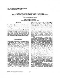
The happy marriage of the techniques of fuzzy logic and neural networks suggests the novel idea of transforming the burden of designing fuzzy logic systems to the training and learning of connectionist neural networks and vice-versa. That is, the neural networks provide connectionist structure and learning to the fuzzy logic systems and the fuzzy logic systems provide the neural networks with a structural framework with high-level fuzzy IF-THEN rule thinking and reasoning. These benefits can be witnessed by the success in applying neuro-fuzzy systems in areas like pattern recognition and control. The research in this thesis addresses neuro-fuzzy systems and their applications especially in character recognition tasks. The neuro-fuzzy systems described in the research presented here are first investigated as whole recognition systems in which performance is compared with corresponding non-fuzzy neural systems or with other neural fuzzy variations. The performance of some neural fuzzy systems is then investigated in which they are used as components of a multi-neural system - either as a neural classifier or as a combiner module. Figure 1.1 illustrates the general structure of the research programme which is described in this thesis. The main motivation for the present research is that, although the benefits of combining fuzzy logic and neural networks are well known and have been widely demonstrated, in this investigation some methods to improve the performance of existing neuro-fuzzy systems are also proposed. In addition, very little has been done to integrate different models of neuro-fuzzy systems (and non-fuzzy neural systems) within a multi-neural system, and this is also addressed in this thesis. This Chapter presents an introduction to the present research. First, a brief introduction to neural networks, fuzzy logic and neuro-fuzzy systems is presented. Then, the organisation of this thesis is presented in which a brief description of the following Chapters is shown, highlighting the main contributions for each Chapter.

Benefits of combining Fuzzy Logic and Neural Networks Levels of investigation

Investigation at an expertlevel, where individual neural classifiers are compa red with corresponding neuro -fuzzy versions and with each other

Investigation in a combinationlevel, where some combina tion methods (fuzzy and nonfuzzy) are investigated


The main aim of this thesis is to investigate the effects of combining fuzzy logic and neural networks, either at an expert-level or at a combination level

Is the use of fuzzy-neural beneficial in a multi-expert system?

Types of combination-level investigations Fuzzy Vs Nonfuzzy methods

Neural Fuzzy Vs fuzzy methods

3

Figure 1.1: General framework of the present research

Neural Vs Nonneural methods


1.2

4

Artificial Neural Networks

The search to model intelligent systems artificially is the main aim of the field of Artificial Intelligence (AI). In this field, there are two major different approaches for modelling human intelligence in machines, which can be characterised as top-down and bottom-up approaches [Haykin, 1998, Lin and Lee, 1996].

• Top-down approach: This approach, also known as symbolic AI, is characterized by a high level of abstraction and a macroscopic view in which a model is first seen as a whole and subsequently broken into sub-models. Classical psychology operates at a similar level and knowledge engineering systems as well as logic programming fall within this approach; • Bottom-up approach: This approach is based on low-level microscopic biological models in which a complex model is composed of several simple units. It is similar to the emphasis of physiology or genetics. Artificial neural networks and genetic algorithms are prime examples of this approach, which originated from modelling of the brain and evolution respectively.

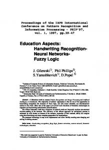
The human brain is believed to consist of approximately 1011 processing units (neurons) with about 1014 connections to each other. Figure 1.2 shows the simplified scheme of such a human neuron. The cell itself is composed of a kernel and the outside is an electrical membrane. Each neuron has an activation level which ranges between a maximum and a minimum. Synapses (connections) exist to increase (exciting) or decrease (inhibiting) the activation through other neurons. These synapses transmit the activation level from a sending neuron to a receiving neuron [M¨ uller et al., 1995]. Despite the slow operation of the individual neurons, the brain can efficiently handle computationally complex tasks, such as pattern recognition, image processing, understanding of natural language, etc [Niklasson and Sharkey, 1994]. Furthermore, incomplete and inconsistent data can be handled by the brain which can learn from experience and is fault tolerant.


5

Axon

Exciting synapses Inhibiting synapses

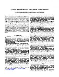
Figure 1.2: Simplified scheme of a human neuron Artificial neural networks, also referred as to connectionist systems or neurocomputing, are a recent generation of information processing systems that are deliberately constructed to make use of some organizational principles that characterize the human brain. The main theme of neural network research focuses on modelling of the brain as a parallel computational device for various computational tasks which have traditionally been difficult to solve using traditional serial computers [Mehrotra et al., 1997]. Artificial neural networks have a massive parallel structure in the form of a directed graph, composed of processing units (neurons) that are linked through connections which may or may not have adjustable weights. Figure 1.3 shows a very simple structure of a neural network, composed of two layers (input and output), each of them composed of three and two processing units, respectively. The following definitions are applied to the structure of a neural network[Haykin, 1998]:

• The nodes of the graphs are called processing units (artificial neurons) which can receive any number of incoming connections (inputs). Also, a neuron can have any number of outgoing connections (outputs), but the signals in all of these must be the same; • The links of the graph are called connections and each connection functions as an instantaneous unidirectional signal-conduction path. The connections may or may not have adjustable weights. In the case of adjustable weights, these determine the

6


Connection

Weight

W ij Input from the external environemnt

Output to the external environment

W li W ik W mi W lk W mk

Processing units

Figure 1.3: The general structure of a neural network effect of the incoming input on the activation level of the neuron; • Input signals to a neural network from outside the network come via connections that originate in the external environment. Outputs from the network to the external environment are connections that leave the network. • Each processing unit performs an information processing operation which can use local memory and/or an input signal and which produces the processing unit’s output signal. The output of a neuron can be passed on either as an input to following neurons or as the neural network’s output. The information processing of a neuron is seen to require two steps, as follows: – The first step is an integration function (typically a dot product) which serves to combine information or activation from the external environment or other neurons into a net input to the neuron. – In the second step, an activation value is output as a function of its net input through an activation function. Identity, step, ramp, piecewise linear, gaussian and sigmoid functions are examples of functions which can be used as an


7

activation function of a neuron;

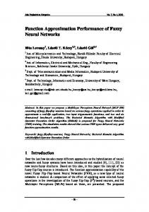
As noted above, the neuron itself computes a very simple function in which a number of input values are received, processed and passed to other neurons as an outgoing value. However, when organised in a highly interconnected structure (neural network), the overall network function becomes much more sophisticated and the network is able to perform complex computational tasks. There are a wide range of neural network models reported in the literature [Haykin, 1998, Lin and Lee, 1996, Mehrotra et al., 1997] which can be differentiated according to the following parameters (Figure 1.4):

• Models of unit processing used (weighted or non-weighted neurons); • Models of interconnections and structure topology (single-layer or multi-layer networks, partially or fully connected networks); • Models of the learning algorithms (supervised or unsupervised learning).

The main advantages of neural networks over conventional systems are their ability to perform nonlinear input-output mapping, generalisation, adaptivity and fault tolerance [Lin and Lee, 1996]. These may be characterised in the following way:

• Nonlinear input-output mapping: Neural networks are able to learn arbitrary nonlinear input-output mappings directly from the training set; • Generalisation: Neural networks can sensibly interpolate input patterns that are new to the network (give an answer based on its own knowledge about the problem given). From a statistical point of view, neural networks can adjust their structure during the learning phase in such a way that they have the ability to generalise to situations that are different from the collected training data without explicit knowledge about the task to be performed; • Adaptivity: Neural networks can automatically adjust their structure (number of neurons or connections) to optimise their behaviour as controllers, predictors, pattern recognizers, decision makers and so on;

8


Artificial Neural Network Models

Single-layer or Multi-layer

e

Neuro

tectur

Archi

n Typ

Learning Method

n Neuro

e

Weighted or Weightless

Supervised or Unsupervised

Figure 1.4: Organisation of neural network models according to their parameters • Fault tolerance: A normal computer system may completely fail in its operation if only a single bit of stored information or a single program statement is incorrect. The performance of a neural network, however, generally degrades gracefully under faulty conditions such as damaged neurons or connections. The inherent fault-tolerance capacity of neural networks stems from the fact that the large number of connections provides much redundancy, since each neuron acts independently of all others and each neuron relies only on local information.

On the other hand, the main disadvantage of neural networks is the broad lack of understanding of how they actually solve a given problem. The main reason for this is that neural networks do not break a problem down into its logical elements, but rather solve it by a holistic approach, which can be hard to understand logically. The main result of neural network learning process is reflected only in a set of weights in which a full understanding of the functioning of the neural network is an almost impossible task. In this case, the only known method of testing the operation of a neural network is to check its


9

performance for individual test cases.

1.3

Fuzzy Systems

Conventional programming languages such as COBOL, FORTRAN or C are based on Boolean logic. Such programming languages are well suited to develop time-sharing, networking and many other systems whose behaviour can be well represented by mathematical models. However, to develop systems that mimic human-like decisions, mathematical models often fall short. Human judgement and evaluation simply does not follow Boolean logic nor any other conventional mathematical discipline. Hence, conventional programming languages, being deeply tied to mathematical logic, are far from efficient when programming and are not sufficient for implementing human-like decision-making processes [Altrock, 1997]. Fuzzy Logic, introduced by Lofti Zadeh in 1965, gives the benefit of enabling systems more easily to make human-like decisions [Zadeh, 1965]. The basis for proposing fuzzy logic was that humans often rely on imprecise expressions like big, expensive or far. But the ”comprehension” of a computer is limited to blackwhite, everything-or-nothing, or true-false modes of thinking. In this context, Lofti Zadeh emphasises that humans easily let themselves be dragged along by a desire to attain the highest possible precision without paying attention to the imprecise character of reality [Jang et al., 1997]. The theory of fuzzy sets, which is based on fuzzy logic, was introduced by Lofti Zadeh in 1965 as a mathematical way to represent vagueness in linguistics and can be considered a generalisation of classical set theory [Lin and Lee, 1996]. The basic idea of fuzzy sets is quite easy to comprehend. In a classical set, which is a collection of distinct objects in which dichotomize the elements of the universe of discourse into two groups, then:

µA (u) = 1, if u is an element of the set A, and µA (u) = 0, if u is not an element of the set A

In using this, an element either belongs to a given set or does not belong.


10

On the other hand, fuzzy sets eliminate the sharp boundaries that divide members from nonmembers in a group. In this case, the transition between full membership and nonmembership is gradual (a fuzzy membership function) and an object can belong to a set partially. The degree of membership is defined through a generalised characterised function called the membership function: µA (u) : U → [0, 1], where U is called the universe and A is a fuzzy subset of U . The values of the membership function are real numbers in the interval [0, 1], where 0 means that the object is not a member of the set and 1 means that it belongs entirely to the set. Each value of the function is called a membership degree. Figure 1.5 shows the principal difference between an ordinary, crisp set and a fuzzy set. Crisp sets are ’clear cut’ while fuzzy sets are graded. In Figure 1.5, for instance, the membership degree to which the two values 14.999 and 15.001 belonging to the fuzzy set ’medium’ are very close to each other, which represents their closeness in the universe, but because of the crisp border between the crisp set ’cool’ and ’medium’, the two values are associated with different crisp sets. The main advantage gained from this approach is the ability to express the amount of ambiguity in human thinking and subjectivity (including natural language) in a comparatively undistorted manner. In this sense, fuzzy logic is appropriate to be used in the following types of problems [Lin and Lee, 1996]: • In problems which are concerned with continuous phenomena (e.g., one or more of the control variables are continuous) that are not easily broken into discrete segments; • In problems where a mathematical model of the process does not exist, or exists but is too difficult to encode, or is too complex to be evaluated fast enough for real-time operation, or involves too much memory on the designated chip architecture; • In problems in which high ambient noise levels must be dealt with or it is important to use inexpensive sensors and/or low-precision microcontrollers;

11


crisp set 'cool'

crisp set 'medium' Fuzzy set 'medium'

0.4

10

15

25

30

Figure 1.5: Representing crisp and fuzzy sets • In problems which involve human interactions and when there is a need to understand human descriptive or intuitive thinking; • In problems in which an expert is available who can specify the rules underlying the system behaviour as well as the fuzzy sets that represent the features of each variable.

With these properties, fuzzy logic techniques find their applications in such areas as control (the most widely applied area), pattern recognition, quantitative analysis, inference and information retrieval [Altrock, 1997]. The main disadvantage of fuzzy systems, however, is that they do not have much learning capability to tune their fuzzy rules and membership functions. Normally, fuzzy rules are decided by experts or operators according to their knowledge or experiences. However, when the fuzzy system model is designed, it is often too difficult (sometimes impossible) for human beings to define all the desired fuzzy rules or membership functions in an optimised way, due to the ambiguity, uncertainty or complexity of the identifying system. Also, fuzzy systems do not have any learning capability in which their fuzzy rules, along with their corresponding membership function, could be automatically tuned in order to reach the desired optimal fuzzy rules and membership functions.


1.3.1

12

Fuzziness is not Probability

Criticisms of fuzzy logic are often based on confusion between the concept of fuzziness and probability. The fundamental difference between them is that fuzziness deals with deterministic plausibility, while probability concerns the likelihood of nondeterministic, stochastic events [Lin and Lee, 1996]. Each morning the weatherman predicts the probability of rain for that day, based on a kind of if-then reasoning, taking into account a number of variables. Probability is a number from zero to one that expresses the certainty that an event will occur. If the probability is zero, then there is a certainty that the event will not occur. If it is one, then there is a certainty that the event will occur. With fuzziness, there is a degree of certainty that something will happen, but when it does, it happens to some degree. When the weatherman says there is a 50 percent chance of rain, he or she seems to mean that there is a 50 percent chance that one drop will fall somewhere in the area. In fuzzy logic, however, one might say that there is a 50 percent probability of a 0.10 thunderstorm. That means that there is a halfway certainty that it will thunder and rain very weakly. According to [Eberhart et al., 1996], one important difference between fuzziness and probability is that probability is only meaningful for things that have not happened yet. Once the event occurs, probability evaporates. The credibility of the weathermen would decrease if they announce the probability of rain yesterday. Yet it is meaningful, and in fact it does happen, for the announcer to talk about the severity of yesterday’s weather. They can suggest that the storm was a ’real bad one’ or ’yesterday was a beautiful day, if you were a duck’. These are ways of saying that, as storms go, this was a real storm: its membership in the set ’storms’ was very high. Probability is meaningless, but fuzzy set membership continues after the event. This discussion does not mean to imply that probability is useless. Probability is appropriate for random-based occurrences. If, when solving a problem, everything needed to calculate probabilities is available and valid, design of a probabilistic system might be a good idea. On the other hand, the more complex a system is, and the more it involves intelligent behaviour, the more likely it is that fuzzy logic will be a good approach, as it has been shown by several authors [Ruspini et al., 1998, Kasabov, 1996, Eberhart et al., 1996, Cox, 1994].


1.4

13

Neuro-Fuzzy Systems

Fuzzy logic [Zadeh, 1965, Ruspini et al., 1998, Cox, 1994] and artificial neural networks [Haykin, 1998, Mehrotra et al., 1997] are complementary technologies in the design of intelligent systems. The combination of these two technologies into an integrated system appears to be a promising path toward the development of Intelligent Systems capable of capturing qualities characterizing the human brain. However, fuzzy logic and neural networks generally approach the design of intelligent systems from quite different angles. Neural networks are essentially low-level, computational algorithms that sometimes offer a good performance in pattern recognition and control tasks. On the other hand, fuzzy logic provides a structural framework that uses and exploits those low-level capabilities of neural networks. Both neural networks and fuzzy logic are powerful design techniques that have their strengths and weaknesses. Neural networks can learn from data sets while fuzzy logic solutions are easy to verify and optimise. Table 1.1 shows a comparison of the properties of these two technologies. In analysing this Table, it becomes obvious that a clever combination of the two technologies delivers the best of both worlds. The integrated system will have the advantages of both neural networks (e.g. learning abilities, optimisation abilities and connectionist structures) and fuzzy systems (humanlike IF-THEN rules thinking and ease of incorporating expert knowledge). In this way, it is possible to bring the low-level learning and computational power of neural networks into fuzzy systems and also high-level humanlike IF-THEN thinking and reasoning of fuzzy systems into neural networks. Thus, on the neural side, more and more transparency is pursued and obtained either by pre-structuring a neural network to improve its performance or by possible interpretation of the weight matrix following the learning stage. On the fuzzy side, the development of methods allowing automatic tuning of the parameters that characterise the fuzzy system can largely draw inspiration from similar methods used in the connectionist community. Summarising, neural networks can improve their transparency, making them closer to fuzzy systems, while fuzzy systems can self-adapt , making them closer to neural networks [Lin and Lee, 1996]. Neural fuzzy systems [Lin and Lee, 1996, Jang et al., 1997] have attracted the growing

14


Neural

Fuzzy

Networks

Logic

Knowledge

Implicit, the system

Explicit, verification and

Representation

cannot be easily

optimisation are very easy

interpreted or modified

and efficient

Trains itself by learning

None, everything must be

from data sets

defined explicitly

Trainability

Table 1.1: Properties of neural networks and fuzzy logic

interest of the researchers in various scientific and engineering areas. Especially in the area of pattern recognition hybrid neuro-fuzzy systems seem to be attracting increasing interest [Alimi, 1997, Baraldi and Blonda, 1998, Meneganti et al., 1998]. There are several ways to combine neural networks and fuzzy logic. Efforts at merging these two technologies may be characterised by considering three main categories: neural fuzzy systems, fuzzy neural networks and fuzzy-neural hybrid systems.

1.4.1

Neural Fuzzy Systems

Neural fuzzy systems are characterized by the use of neural networks to provide fuzzy systems with a kind of automatic tuning method, but without altering their functionality. One example of this approach would be the use of neural networks for the membership function elicitation and mapping between fuzzy sets that are utilized as fuzzy rules. This kind of combination is mostly used in control applications. Examples of this approach can be found in [Wang and Mendel, 1992, Nomura et al., 1992, Nauck, 1994, Shi and Mizumoto, 2000b, Shi and Mizumoto, 2000a, Yager and Filev, 1994, Cho and Wang, 1996, Ichihashi and T¨ uksen, 1993]. Figure 1.6 illustrates an example of a neural fuzzy system. In this example, the neural network simulates the processing of a fuzzy system in which the neurons of the first layer are responsible for the fuzzification process. The neurons of the second layer represent the fuzzy words used in the fuzzy rules (third layer). Finally, the neurons of the last layer


Fuzzification

Inference

15

Defuzzification

Figure 1.6: An example of the mapping of a neural network to a fuzzy logic system are responsible for the defuzzification process. In the training process, a neural network adjusts its weights in order to minimise the mean square error between the output of the network and the desired output. In this particular example, the weights of the neural network represent the parameters of the fuzzification function, fuzzy word membership function, fuzzy rule confidences and defuzzification function respectively. In this sense, the training of this neural network results in automatically adjusting the parameters of a fuzzy system and finding their optimal values.

1.4.2

Fuzzy Neural Networks

The main goal of this approach is to ’fuzzify’ some of the elements of neural networks, using fuzzy logic. In this case, a crisp neuron can become fuzzy. Since fuzzy neural networks are inherently neural networks, they are mostly used in Pattern Recognition Applications.


16

Examples of this approach can be found in [Baraldi and Blonda, 1998, Dagher et al., 1998, Pal and Mitra, 1992, Canuto et al., 1999b, Canuto et al., 1999a, Carpenter et al., 1992b, Carpenter and Markuzon, 1998, Carpenter et al., 1991a]; In [Lin and Lee, 1996], for instance, a neural network composed of fuzzy neurons is presented. In these fuzzy neurons, the inputs are non-fuzzy, but the weighting operations are replaced by membership functions. The result of each weighting operation is the membership value of the corresponding input in the fuzzy set. Also, the aggregation operation may use any aggregation operators such as min and max and any other t-norms and t-conorms [Lin and Lee, 1996] In this thesis, fuzzy neural networks will be used in which some of the elements of some neural networks will have some form of fuzzification.

1.4.3

Fuzzy-Neural Hybrid Systems

In this approach, both fuzzy and neural networks techniques are used independently, becoming, in this sense, a hybrid system. Each one does its own job in serving different functions in the system, incorporating and complementing each other in order to achieve a common goal. This kind of merging is application-oriented and suitable for both control and pattern recognition applications [Lin and Lee, 1996].

1.5

Organisation of the Thesis

The remainder of this thesis has been divided into six Chapters. The organisation of this work is as follows:

Chapter 2 Fuzzy Multi-Layer Perceptron

In this Chapter, a modified version of the fuzzy multi-layer perceptron model is proposed. The proposed model makes use of membership (similarity) values as a way to define the fuzzy desired output vector as well as adding a parameter to the


17

updating equation in order to take into account the degree of ambiguity of an input pattern during the learning phase. In addition, experimental testing is performed in order to investigate the benefits of using the proposed techniques within a multi-layer perceptron model. The main contribution of this Chapter is the proposal of new techniques to improve the performance of multi-layer perceptrons. The comparative analysis shows a significant improvement of the proposed fuzzy multi-layer perceptron over its corresponding non-fuzzy version.

Chapter 3 RePART: A Fuzzy ARTMAP with a Reward/Punishment Process

In this Chapter, RePART, a proposal for a variant of fuzzy ARTMAP is analysed. Essentially, RePART is a more developed version of the simpler fuzzy ARTMAP which employs additional mechanisms to improve performance and operability, such as a reward/ punishment process, an instance counting parameter and variable vigilance parameter. The idea of using a reward/punishment process is to improve the performance of fuzzy ARTMAP networks. The idea of using a variable vigilance parameter is to decrease the complexity (category proliferation problem) of fuzzy ARTMAP models when used in applications with a large number of training patterns. A comparative analysis of the proposed model (without using variable vigilance parameter) and other fuzzy ARTMAP-based models (fuzzy ARTMAP and ARTMAPIC) shows an improvement achieved by RePART over the other models, and this is the main contribution of this Chapter.

Chapter 4 An Analysis of RePART, Fuzzy MLP and Radial RAM Networks

Once the two main neuro-fuzzy models are introduced, it is important to compare the performance of these two models, which is the subject of this Chapter. Also, a nonfuzzy neural model, radial RAM, is used in this Chapter. In the RePART network, the use of a variable vigilance parameter is also analysed in order to smooth the


18

category proliferation problem of ARTMAP-based models. The comparative analysis shows that when not using variable vigilance values, the RePART model delivered a better performance than the other two models when a small number of training patterns was employed. However, when using a large number of training pattern, RePART delivers the worst performance. On the other hand, when using variable vigilance values, RePART delivers a similar performance to that of the fuzzy multi-layer perceptron and a better performance than radial RAM. Moreover, the use of variable vigilance causes a reduction of around 30% in the size of the RePART architecture. These are the main contributions of this Chapter.

Chapter 5 Combination of Neural Classifiers

This Chapter presents a survey of combination methods for neuro-fuzzy and nonfuzzy neural experts, including fuzzy, neural and neuro-fuzzy methods. Within this Chapter, the steps needed in the design of a multi-neural system are described. A general classification of the combination methods along with the description of some combination methods, followed by a description of some methods of using fuzzy set theory as a combination tool are also presented as well as the use of some learning strategies for multi-neural systems. Also, the Chapter describes some ways to calculate confidence measures to be used in a multi-neural system. The focus of this survey in fuzzy and neuro-fuzzy combination methods is the main contribution of this Chapter, since very little work has been reported to date in combining different types of neuro-fuzzy and non-fuzzy neural systems using fuzzy, conventional and neuro-fuzzy combiners.

Chapter 6 Experimental Testing in a Multi-neural System

In this Chapter, an analysis of the performance of some combination schemes applied to a hybrid multi-neural system composed of neural and fuzzy neural networks is investigated. Essentially, the set of experiments is divided into three parts. The first


19

part investigates the performance of a hybrid multi-neural system in comparison with non-hybrid multi-neural systems. The second part analyses the benefits of using confidence measures in combination methods while the final part investigates the benefits of using fuzzy theory set as a combination mechanism. The main conclusions of the experiments are that firstly the use of the hybrid system resulted in an improvement over the performance of non-hybrid systems. Also, not only does the introduction of a confidence-based decision improve classification performance, but also that combining confidence measures results in yet a further improvement in all cases. Finally, the use of neuro-fuzzy combiner improved the performance of the multi-neural system over neural network and fuzzy combiners. These are the main contributions of this Chapter.

Chapter 7 Conclusions and Further Researchs

In this Chapter, a summary of this work, along with some concluding remarks and suggestions for further research are given.

20

Chapter 2

Fuzzy Multi-Layer Perceptron

This Chapter presents a modified fuzzy multi-layer perceptron model which uses, as its basis, the implementation developed in [Pal and Mitra, 1992]. The model is suitable for tasks in a binary domain. The proposed model makes use of membership (similarity) values as a way to define the fuzzy desired output vector as well as adding a parameter to the updating equation in order to take into account the degree of ambiguity of an input pattern during the learning phase.

21


2.1

Introduction

The multi-layer perceptron (MLP), using the backpropagation learning mechanism, is the most widespread neural network encountered in the literature [Mehrotra et al., 1997] and it has been employed in a wide range of applications such as pattern recognition [DimlaSr. and Lister, 2000, Jeong et al., 2000, Zhang et al., 1998], medical image analysis [Guler et al., 1998, Sheppard et al., 1999] and forecasting [Indro et al., 1999]. Essentially, the MLP is a feedforward multi-layer network which uses a supervised error-based learning mechanism. That is, it uses a mechanism that modifies the weights of the network in order to minimise the mean squared error between the desired and actual outputs of the network [Rumelhart et al., 1986]. The fuzzy multi-layer perceptron is an implementation of fuzzy set theory in a multi-layer perceptron network [Pal and Mitra, 1992, Keller and Hunt, 1985]. In other words, it is the result of the direct fuzzification either at a network-level, learning-level or a networklearning-level of the multi-layer perceptron. There exists a vast

literature

on combining

fuzzy set theory [Ruspini et al., 1998,

Zadeh, 1965] and the multi-layer perceptron [Haykin, 1998, Mehrotra et al., 1997], such as in [Nauck, 1994, Stoeva and Nikov, 2000, Pal and Mitra, 1992, Keller and Hunt, 1985, Sural and Das, 1999, Shi and Mizumoto, 2000a, Shi and Mizumoto, 2000b]. In this Chapter, a network-learning-level fuzzification of the multi-layer perceptron is proposed in which the following mechanisms have been added to the multi-layer perceptron operability.

• Fuzzy desired output: In this mechanism, fuzzy concepts are employed in order to calculate the desired output of patterns which are presented to the MLP neural model during the learning and recalling phases; • Degree of ambiguity: In this mechanism, a parameter which takes into account the degree of ambiguity of the input pattern has been added to the weight update equation.

The proposed fuzzy multi-layer perceptron model uses, as its basis, the implementation


22

developed in [Pal and Mitra, 1992] and it is suitable for applications in the binary domain (the model proposed in [Pal and Mitra, 1992] is suitable for applications in a grey-scale or colour domain). This Chapter is divided as follows. Firstly, a brief description of the conventional multilayer perceptron is presented. Secondly, a description of the fuzzy multi-layer perceptron proposed in [Pal and Mitra, 1992] is presented, together with the proposed modifications in order to make fuzzy MLP suitable for tasks in the binary domain. Subsequently, the results of some experiments that have been performed to investigate the performance of the proposed model in comparison with the original multi-layer perceptron are presented.

2.2

Multi-Layer Perceptron

The perceptron and other one-layer networks have been shown to be seriously limited in their capabilities [Minsky and Papert, 1969]. Feedforward multi-layer networks, such as the multi-layer perceptron, with non-linear node functions, can overcome these limitations and can be applied to a wide range of tasks [Guler et al., 1998, Indro et al., 1999, DimlaSr. and Lister, 2000, Jeong et al., 2000, Sheppard et al., 1999]. The learning mechanism generally applied to this network is called backpropagation and was first proposed by Werbos [Werbos, 1974]. However, it was largely ignored by the scientific community until the 1980’s, when it was independently rediscovered by Parker [Parker, 1985], LeCun [Cun, 1998] and in its most popular version by Rumelhart, Hinton and Williams [Rumelhart et al., 1986]. The backpropagation learning algorithm assumes a feedforward neural network architecture such as a multi-layer perceptron. In this architecture, nodes are partitioned into layers - numbered 0 to L - in which the initial layer - layer number 0 - is the input layer, the final layer (number L) is the output layer and the other layers situated between the initial and the final layers - from layer number 1 to (L-1) - are called the hidden layers. Figure 2.1 shows a typical example of a multi-layer perceptron architecture which is composed of an input layer, two hidden layers and an output layer. The backpropagation algorithm is a generalisation of the least mean squared algorithm

23


Hidden layer 2 Input layer Hidden layer 1

Output layer

Figure 2.1: The general structure of multi-layer perceptron that modifies the weights of a neural network in order to minimise the mean squared error between the desired and current outputs of the network by a gradient descent method. As a supervised learning algorithm, inputs as well as desired outputs are known. Essentially, the backpropagation learning process is composed of two steps, corresponding to a feedforward and a backward step, as follows:

• Feedforward step: During this phase, an input pattern is presented to the input layer neurons that pass them on to the first hidden layer. The hidden layer nodes compute a weighted sum of their inputs, pass the sum through their activation function and present the result to the next hidden layer. This process is repeated until the result is presented to the output layer of the network whose result is the actual output of the neural network. • Backward step: Once the output of the network is calculated, the mean squared error between the desired and actual outputs of the network is defined. Subsequently, this error is back-propagated and is used as basis in order to modify the weights of the network [Rumelhart et al., 1986, Haykin, 1998].


2.3

24


As mentioned above, there is a vast literature on combining fuzzy set theory [Zadeh, 1965, Ruspini et al., 1998] and the multi-layer perceptron [Haykin, 1998, Mehrotra et al., 1997], such as in [Shi and Mizumoto, 2000a, Stoeva and Nikov, 2000, Shi and Mizumoto, 2000b, Pal and Mitra, 1992, Sural and Das, 1999, Keller and Hunt, 1985, Nauck, 1994]. Essentially, the combination of these two technologies can be achieved in three different ways, which are network-level fuzzification, learning-level fuzzification and networklearning-level fuzzification, as follows: • network-level fuzzification: In this method, the process of fuzzification occurs in the structure of the multi-layer perceptron model, such as in neurons (and weights) and/or in the whole architecture as well as in the desired output. – Neurons and whole architecture: In most cases, simulation of the behaviour of a fuzzy system is performed in which neurons represent fuzzy functions with parameters (weights) or fuzzy rules. The layers of neurons represent the set of rules. In these cases, a conventional gradient descent backpropagation algorithm is employed in order to update and tune the parameters of the fuzzy system. The main aim of this approach is the optimisation of fuzzy systems. Normally, fuzzy rules are decided by experts or operators according to their knowledge or experiences. However, when the fuzzy system model is designed, it is often too difficult (sometimes impossible) for human beings to give desired fuzzy rules or membership functions, due to the ambiguity, uncertainty or complexity of the identifying system. For this reason, it is natural and necessary to generate or tune fuzzy rules by some learning technique. Fuzzy rules can be generated or tuned for constructing an optimal fuzzy system model by the backpropagation algorithm. This approach has been widely used, and examples can be found in [Shi and Mizumoto, 2000b, Cho and Wang, 1996, Wang and Mendel, 1992, Ichihashi and T¨ uksen, 1993, Yager and Filev, 1994, Shi and Mizumoto, 2000a, Nomura et al., 1992, Nauck, 1994]; – Desired output: In this approach, the desired output vector is fuzzified in or-


25

der to represent the degree of membership (similarity) of the input pattern to each output class (see [Pal and Mitra, 1992] as well as in this Chapter Section 2.3.1.2); • learning-level fuzzification: In this method, the process of fuzzification occurs in the learning algorithm, preserving the multi-layer perceptron architecture (also known as fuzzy backpropagation). In this case, the learning fuzzification tries to improve some weak points of the backpropagation method, achieving increasing convergence rate [Stoeva and Nikov, 2000], improving accuracy [Hwang et al., 1997], decreasing influence of ambiguous training patterns (in this Chapter and in [Canuto et al., 1999a] as well as in [Keller and Hunt, 1985]); • network-learning-level fuzzification: In this method, the process of fuzzification occurs in the structure of the multi-layer perceptron model as well as in the backpropagation learning method. One example of this method is when the structure is adjusted as a fuzzy control system and its learning procedure is fuzzified in order to better tune its fuzzy rules and parameters. Examples of this method can be seen in [Shi and Mizumoto, 2000b].

In this Chapter, a network-learning-level fuzzification is analysed in which fuzzy concepts are employed in order to define the desired output vector (network-level fuzzification) and a fuzzy parameter is added to the updating equation during the learning process (learning-level fuzzification).

2.3.1

Desired Output Vector

Usually, in the conventional MLP [Haykin, 1998, Rumelhart et al., 1986], the number of nodes in the output layer corresponds to the number of pattern classes occurring in the task to be performed. In such a network, the winner-takes-all method can be used during the learning and recalling phases of the network. Winner-takes-all is a method which assigns 1 to the winning element and 0 to the other elements. During the recalling phase, winner-takes-all is used in order to define the winning neuron - the neuron which represents the network’s prediction about the class to which the input pattern belongs -, assigning 1 to this neuron and 0 to the other neurons.

26


The winner-takes-all process is applied during the learning process in order to define the desired output vector. In the desired output vector, the class to which the input pattern belongs is assigned the value 1, and the other classes are assigned the value 0. This is called a crisp desired output. The output of the networks is compared with the desired output in order to calculate the mean square error, which is then back-propagated to modify the weights of the network. In real-world problems, however, the data are generally ill-defined, with overlapping or fuzzy class boundaries. There are some patterns that can have non-zero membership (similarity) to two or more pattern classes. In the Pattern Recognition field, for instance, it is very common that an input pattern has a degree of similarity (non-zero membership) to more than one class. Figure 2.2 is a simple example of patterns which belong to the overlap region and have non-zero similarity with both classes (A and B).

Class A

Class B Overlap Region

Figure 2.2: An example of a two-class space In the conventional multi-layer perceptron, this multiple similarity is not considered since crisp desired output (only the winner class is considered and with maximum similarity 1) is assigned and used during training and recalling. In order to consider the membership values of every class, it would seem very promising to incorporate fuzzy concepts in the calculation of the desired output [Pal and Mitra, 1992, Canuto et al., 1999a]. Unlike the conventional multi-layer perceptron, the fuzzy multi-layer perceptron can clamp desired membership values (calculated incorporating fuzzy concepts) to the output nodes during the training phase instead of choosing binary values as in a winner-takes-all method


27

[Pal and Mitra, 1992]. Subsequently, the errors may be back-propagated with respect to the exact similarity which is reflected in the desired output - fuzzy desired output. The use of fuzzy desired output enables the multi-layer perceptron model to more efficiently classify fuzzy data with overlapping or fuzzy class boundaries. In addition, the fuzzy MLP can be applied in any task for which the conventional MLP is used, principally the three areas which may be characterised as pattern recognition [Jeong et al., 2000, DimlaSr. and Lister, 2000, Zhang et al., 1998], medical image analysis [Guler et al., 1998, Sheppard et al., 1999] and forecasting [Indro et al., 1999]. In this Chapter, the use of fuzzy desired outputs in the multi-layer perceptron model will be investigated in the pattern recognition area, focusing on grey-scale and binary images.

2.3.1.1

Desired Output for Gray-Scale Images

As mentioned before, unlike the conventional multi-layer perceptron, each desired output of the fuzzy multi-layer perceptron lies in the range [0,1] and refers to the degree of membership (or similarity) of the input pattern to its corresponding output pattern class. In [Pal and Mitra, 1992], a method to employ fuzzy concepts in order to calculate the fuzzy desired output was proposed. This method is suitable to grey-scale images and uses as its basis two parameters, which are the following:

1. Mean vector of the training set; 2. Standard deviation of the training patterns.

According to [Pal and Mitra, 1992], in order to derive the fuzzy desired output, the following steps are performed:

1. Calculate the weighted distance between the input pattern and each pattern class (k = 1, ..C), taking into account the mean and standard deviation of the training patterns. The weighted distance of the training pattern i to the kth class is defined by:

28

Fuzzy Multi-Layer Perceptron n xij − µkj Dk = σkj

(2.1)

j=1

where: xij is the value of the jth pixel of the input pattern i; µkj is the value of the jth pixel of the mean vector of the kth class; σkj is the value of the jth pixel of the standard deviation vector of the kth class; n is the size of the pattern vector. 2. Once the weighted distance is defined, the membership values for each class (µk for k = 1, ..C) are calculated using the following equation:

1 fe

µk (Dk ) = 1+

(2.2)

Dk fd

where: Dk is the weighted distance of the input pattern to class k; fe and fd are fuzzy parameters.

These two fuzzy parameters (fe and fd ) control the amount of fuzziness for this class membership set. The idea behind the membership function is that the higher the distance of an input pattern from a class k, the less similar this pattern is to class k and, as a consequence, the lower its membership value for that class.

2.3.1.2

Proposed Desired Output Vector

Usually the two parameters used in the above method (mean and standard deviation) are applied to domains with a wide range of values. For instance, standard deviation defines the deviation of a given value in relation to the other values in the domain. In the binary domain, however, as there are only two possible values, 0 and 1, it is meaningless to employ the standard deviation and mean since there is just one value to compare with the given value.

29


An alternative way of computing the fuzzy desired output for the fuzzy multi-layer perceptron is proposed in this Section and in [Canuto et al., 1999a]. In this alternative method, instead of standard deviation and mean, two other parameters are employed, which are prototype and variability of a class.

• Prototype of a class: This parameter defines the frequency of occurrence of binary values in the training patterns for each pattern within the training set. In other words, it calculates the distribution of values in the training patterns and is determined on a pixel by pixel basis. The equation which calculates the prototype parameter can be defined as follows. L

Pik =

Tij

j=1

L

,

(2.3)

where Pik is the prototype of the ith pixel of the class k, k = 1,..,C where C is the number of classes. The prototype is calculated pixel by pixel (i = 1,2,..M); Tij is the ith pixel of the training pattern in question (j); M is the number of pixels of a pattern; L is the number of training patterns. As can be seen from equation 2.3, values of this parameter (P ) lie within the range [0,1] in which values close to ’1’ imply that, in that particular pixel, more ’1’ values were presented. A similar process occurs with values close to ’0’, indicating the occurrence of ’0’ values presented in the training pattern. The ideal values for the prototype are values close to the two extremes - either close to 1 or close to 0 - because that would indicate a dominance of a value during training. For instance, values around 0.5 defines no dominance since the value 0 has been presented as many times as the value 1. • Variability of a class: This parameter has a fundamental role in the process of calculating the fuzzy desired output and is concerned with the variations of prototype values for each pixel in the set of the training patterns. As the prototype measure

30


represents a mean sample of a class, variations of the prototype (Variability) define intra-class variation of the training set. Variability takes into account the prototype (eqn. 2.3) and it is defined as follows. M

Vk =

(0.5 − Pik )2

i=1 M 4

,

(2.4)

where Pik is the ith pixel of the prototype of the class k, k = 1,..,C; M is the number of pixels of the prototype. In using prototype values close to the extremes - either close to 0 or 1 (ideal values for the Prototype parameter), the numerator part of the above equation will be close to ((±0.5)2 = 0.25), in which multiplied by M results in a value close to (M/4), that will provide a variability close to 1 when divided by (M/4). As already mentioned, a variability close to one means that there is a consensus (not much variation) in the prototype of this class. On the other hand, when variation in prototype is high, Pik will lie around 0.5 for the majority of the pixels, leading to a numerator part close to 0 and, as a consequence producing a variability close to 0. As can be seen from equation 2.4, the Variability parameter reflects the variations of a pattern class in an inverse order. Values of Variability close to 1 mean consensus among the training patterns and low degree of variation in the training set. On the other hand, values of Variability close to 0 means a high degree of variations in the training set. The main reason for using the inverse order is to facilitate its application in the membership function equation (eqn. 2.7).

The definition of these two parameters (prototype and variability) is performed before the training process begins and takes into account the whole training set. During the training and recalling phases, for each input pattern which is clamped to the input layer, it will be compared with the parameters of its corresponding class in order to derive its fuzzy desired output.

31


The steps to calculate the fuzzy desired output of an input pattern are very similar to those suitable for grey-scale images and can be defined by the following process:

1. Calculate the weighted distance (Dk ) of the input pattern to the pattern classes, taking into account the squared error between the input pattern and the prototype of a class. The main aim of the weighted distance is to calculate the distance of the input pattern and the pattern classes and this is defined by:

Dk =

1 Ek C l=1

f

1 El

,

(2.5)

where:

Ek =

M

(Xi − Pik )2 ,

(2.6)

i=1

where Pik is the ith pixel of the prototype of class (eqn. 2.3) k, k = 1,..,C where C is the number of classes; Xi is the ith pixel of the input pattern under consideration; M is the number of pixels comprising the patterns; f is the fuzziness similarity which determines the rate of decrease of the weighted distance of the input pattern according to its error (usually its value is in the interval [0,1]). In the weighted distance equation (equation 2.5), the smaller the error between the input pattern and the prototype of the class k, the higher its value. In other words, the more similar the input pattern is to a class k, the higher is its corresponding weighted distance. 2. Calculate class membership values for the input pattern which takes into account the weighted distance of the closest class, the other weighted distances and its corresponding variability. This is defined as follows:

32


µk =

Zk Z

exp ,

(2.7)

Zk = Dk × Vk ,

(2.8)

where:

and Vk is the variability of the class k, k = 1,..,C C is the number of classes; Dk is the weighted distance of the input pattern to the class k; exp is a fuzzy parameter which defines the width of the membership function; Z is the similarity of the closest class (biggest value) calculated for the input pattern. In equation 2.8, a reduction process of the weighted distance is applied in which classes with high variability (low Vk ), have their weighted distance decreased. On the other hand, weighted distances of classes with low variability (high Vk ) will be kept almost unchanged. Subsequently, among the weighted distances, the highest one - the most similar class (Z) - is chosen and the class membership values are calculated (equation 2.7), taking into account the highest weighted distance, the other weighted distances and a fuzzy parameter which defines the width of the membership function.

As already noted, the process of deriving fuzzy desired outputs presented above is suitable for tasks within binary domains. The process takes into account two new parameters prototype and variability - as well as the squared error between the input pattern and the prototype of a class, a reduction expression and two fuzzy parameters. These fuzzy parameters define the rate of decrease of the weighted distance and the width of the membership function.


2.3.2

33

The Process of Updating the Weights

The way to learn information in the conventional multi-layer perceptron network is through the minimisation of least mean square (LMS) error in output vectors (network and desired output) and it is known as a gradient descent method. The minimisation of LMS is achieved through the update of the weights of the network. In order to calculate the new weights of the network, a momentum updating equation is used, defined as follows [Haykin, 1998]:

Wij (t + 1) = Wij (t) + ηγi δi (t + 1) + αWij

(2.9)

where:

Wij (t + 1) is the new weight of the connection from the ith neuron to the jth one; Wij (t) is the old weight of the connection from the ith neuron to the jth one; η is the learning rate; δi is the parameter that is calculated according to the LMS error and the layer in which the neuron is found; γi is the output of the neuron i; α is the momentum parameter; Wij is the change in the weight during the last iteration The momentum updating equation updates the weights of a network based on their previous weights according to a certain learning rate together with the update value from the previous iteration according to a momentum parameter. In the weight update process presented above (equation 2.9), each training pattern has the same importance in adjusting the weights. However, there are patterns that are in overlapping areas and that are mainly responsible for misclassification (erratic behaviour). In the momentum equation, this factor is not considered and ambiguous training patterns have the same influence in the updating of the weights as unambiguous patterns.


34

One way to improve the performance of the algorithm is to consider the amount of correction in the weight vector produced by the input pattern. Here, the amount of correction is defined by the degree of ambiguity of a pattern in which the more ambiguous an input pattern, the less correction in the weight. Therefore, ambiguous patterns should have less influence in the vector updating process. The degree of ambiguity is an additional parameter to be used in the proposed fuzzy multilayer perceptron which was not employed in the model proposed in [Pal and Mitra, 1992]. This idea is similar to the one in [Keller and Hunt, 1985], which was based on a two class partition and here it is extended to an N class partition. The degree of ambiguity (A) can be defined as follows.

A = (µi (x) − µj (x))m

(2.10)

where:

µi (x) is the membership value of the top class i; µj (x) is the membership value of class j, the second highest one; m is an enhancement/reduction fuzzy parameter.

The degree of ambiguity is calculated taking into account the difference between the membership value of the top class and the second highest class membership value. The enhancement/reduction fuzzy parameter m either enhances (m < 1), maintains (m = 1) or reduces (m > 1) the influence of the ambiguity of a training pattern as well as the strength of this enhancement/reduction. The degree of ambiguity is, then, used as a parameter in the weight updating equation (see equation 2.9) in the second term of that equation, along with the learning rate (η) and the output of the neuron. The new weight equation will be:

Wij (t + 1) = Wij (t) + (µi (x) − µj (x))m ηδi (t + 1)γi (t + 1) + αWij

(2.11)


35

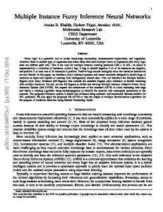
The new parameter (the underlined part of the eqn. 2.11), when an input pattern is ambiguous, has high similarity (membership value) to more than one class. Therefore, its degree of ambiguity value is low, decreasing the level of correction of the weight vector. In other words, the problem of ambiguous patterns having much influence in the weight updating process is avoided. The more ambiguous a training pattern, the less its influence on the weight updating equation. Figure 2.3 depicts the learning processing of the fuzzy multi-layer perceptron presented in this Chapter, including the derivation of fuzzy desired output and the addition of the degree of ambiguity.

2.3.3

Learning Strategy

In the perceptron-based models, one training iteration contains one presentation of the whole training set in a chosen order. Several learning strategies can be applied to a perceptron neural network, the main ones being learning by pattern, learning by block and learning by epoch [Torresen, 1997].

• Learning by pattern: In this strategy, the process of updating the weights of the network occurs after each training pattern has been presented. In other words, after each training pattern has been presented, the updating of the weights of a networks occurs in order to adjust the weights of the network to better represent the training pattern most recently presented; • Learning by block: In this strategy, the process of updating the weights of the network occurs after a subset of the training pattern has been presented. In other words, after N training patterns have been presented, the updating of the weights of a network occurs; • Learning by epoch: In this strategy, the process of updating the weights of the network occurs after all training patterns have been presented.

Pre-Training

Training Fuzzy Multi-Layer Perceptron

Forward step

Backward step

Calculating fuzzy desired output Calculate Degree of ambiguity

Error

Calculate Prototype

Calculate Variability of a class

I N P U T P A T T E R N

Weighted distance

membership values

MLP Neural Network

Calculate the error between the output of the network and the fuzzy desired output

Update the weight vector

Training Set

36

Figure 2.3: The learning process of fuzzy multi-layer perceptron


37

In the perceptron neural networks presented in this Chapter, the first strategy - learning by pattern - is applied as their learning strategy. Now that the proposed modifications have been presented, a comparative analysis will be performed in which the proposed fuzzy multi-layer perceptron and a conventional MLP will be applied to a handwritten and machine-printed numeral recognition task in order to analyse the comparative performance of these networks. This comparative analysis will be described in the next Section.

2.4

Comparative Analysis

It is interesting to compare the fuzzy MLP with the conventional MLP in order to investigate the performance of the proposed network and this analysis is described in this Section. It is important to emphasise that although the fuzzy MLP proposed in this Chapter is based on the fuzzy MLP proposed in [Pal and Mitra, 1992], it is not possible to carry out a comparative analysis between these two fuzzy neural networks since they are suitable for applications in different domains (the fuzzy MLP model proposed in this Chapter is suitable for binary domains while the model proposed in [Pal and Mitra, 1992] is suitable for grey-scale or colour domains). Due to this fact, this comparative analysis will investigate the benefits of using fuzzy concepts within the conventional multi-layer perceptron training process. This Section will thus describe a comparative analysis between the fuzzy MLP and the conventional MLP, using machine-printed and handwritten character databases. The comparative analysis will be addressed systematically varying the following parameters:

• Size of the training set; • Training time (number of iterations during training); • Neural network configuration (number of layer and number of neurons within a layer).


38

A handwritten and machine-printed numeral recognition task will be investigated. The machine-printed database contains characters extracted from post-codes supplied by the British Post Office and was compiled in-house by the University of Kent. The handwritten database was compiled in-house by the University of Essex. The neural networks were trained with different numbers of training patterns and tested with 1000 different patterns - 100 for each class. In order to avoid atypical data partitions, the training patterns were randomly chosen and the neural networks were trained using the selected patterns. This process was repeated ten times and the performance levels reported are mean values taken from these processes. Based on initial experiments, the following configuration is chosen as the most suitable to the starting point for the comparison: 3 layers with 384-100-10 neurons per layer respectively (where 384 is the length of the input pattern and 10 is the number of classes to be recognisee), 250 training patterns - 25 for each class, 50 epochs for the training phase. Although the task to be performed in both databases is the same - character recognition - the databases are different from each other and pose different degrees of difficulty in the recognition process. For the above reason, different settings have been used for the fuzzy parameters (initial testing showed that the setting for the first database is not appropriate for the second one). An initial experiment showed that the values for the fuzzy parameters which produced the highest recognition rate in the fuzzy MLP (chosen configuration) employed in the machine-printed database are: Fuzziness Similarity (f ) (equation 2.5) = 0.75, Exponential fuzzy (exp) (equation 2.7) = 0.5 and the enhancement/reduction fuzzy parameter (M ) (equation 2.11) = 1. For the handwritten database, the chosen configuration was: Fuzziness Similarity = 0.85, Exponential fuzzy = 0.45 and the enhancement/reduction fuzzy parameter = 0.75.

2.4.1

Size of the Training Set

The size of the training set defines the number of patterns which will be presented to the network during the training phase. In this subsection, the comparative behaviour of the fuzzy and the conventional MLP will be analysed, with the following sizes of the training

39


Machine-printed character

handwritten character

Training patterns

conventional

Fuzzy

conventional

Fuzzy

per class

MLP

MLP

MLP

MLP

10

73.2%

82.4%

38.8%

65%

25

84.8%

91.1%

59.6%

82.7%

50

88.9%

93.3%

72.5%

88.3%

75

94.2%

97.9%

76.8%

91.2%

100

94.9%

98.1%

79.4%

92.1%

150

96.3%

98.6%

82.1%

93.7%

Table 2.1: Comparative analysis of performance with variation of the size of training pattern set

set: 10 (for each class), 25, 50, 75, 100 and 150. Table 2.1 shows the performance of the fuzzy and conventional MLP according to variations in the size of the training set, using machine-printed and handwritten character databases.

2.4.1.1

Machine-Printed Character Database

First of all, it is important to verify the performance of the neural networks individually with variation of the size of training set pattern (first and second columns of Table 2.1). In this analysis, it is possible to state that both neural networks, the fuzzy MLP and the conventional MLP, have a similar pattern of performance with the recognition rate of both networks starting at a low rate and improving as the size of the pattern training set increases. This is followed by a stabilisation. This is due to the fact that when using a few patterns, there is not enough data in order to obtain a good measure of the class distribution and therefore the performance is poor. As the number of training patterns increases, more data relating to the classes is provided and consequently the performance improves. Comparing the difference in performance between the fuzzy MLP and the conventional MLP, it starts high (9.2% when using 10 training patterns per class) and it decreases as


40

the size of the training set increases (2.3% when using 150 training patterns per class). This is significant since it is possible to say that, for the analysed task, the fuzzy MLP is easier to stabilise with fewer training patterns. This improvement in the performance of fuzzy MLP (4.85% on average) is due to the fact that the variability of the data sample is better represented using non-zero membership values. In a numeral recognition task, it is very common that a training pattern has nonzero similarity with more than one class (patterns from classes 3 and 8, for instance, are similar and a pattern which belongs to one of these classes can have non-zero similarity to the other class). This multiple similarity is reflected in non-zero membership values (fuzzy desired output), which makes the training process stabilise with fewer training patterns. In using a large training set, the stabilisation of the fuzzy MLP training is easier than conventional MLP. However due to the high number of training patterns, this stabilisation is not as easy as when using a small number of training patterns. The improvement in performance of the fuzzy MLP is an important point because sometimes it is not possible to obtain a large number of training patterns. To summarise the above observations, the performance of the neural networks started low and then increased to become stable. It can be deduced, analysing Table 2.1, that a training set with 75 patterns per class represents the best result considering the tradeoff between performance and time processing. The main reason is that it has one of the highest recognition rates and time processing of the training phase is reasonable when compared with the time processing of networks using larger patterns in the training set, such as 150 patterns per class. Therefore, in subsequent experiments, the size of the training set is 75 patterns per class.

2.4.1.2

Handwritten Character Database

In analysing the last two columns of Table 2.1, a similar performance pattern is observed for both neural networks, starting with a low recognition rate, increasing according to the increase of the size of the training set and subsequently stabilising. The magnitude of the difference between the two networks started high (26.2% with 10 training patterns per class) and decreased according to the increase of the size of the training set, reaching an


41

improvement of 11.6% when using 150 training patterns per class. It can be concluded from Table 2.1, that the best tradeoff between performance and time processing was obtained with 75 training patterns per class. Although higher recognition rates were reached when using more training patterns (100 and 150 training patterns per class), the cost (time processing) involved in the training process of using more training patterns is high. Therefore, for the handwritten character database, from now on, 75 training patterns per class are used in all subsequent experiments.

2.4.1.3

Discussion

Comparing the performance of the networks with the two databases, three main observations that can be made:

1. There is a decrease in the level of recognition performance for the handwritten characters compared with machine-printed characters. This is caused by the wider range of variability of handwritten characters sample data compared with machineprinted ones, which poses a higher degree of difficulty in the recognition process; 2. The increase of the training set size has a similar effect in the pattern of performance of the neural networks for both machine-printed and handwritten numerals, but at different levels; 3. The most important observation is that the magnitude of difference in performance between fuzzy and non-fuzzy models using handwritten database is higher than machine-printed task, which was, on average, 4.85% while the difference for handwritten characters was, on average, 17.1%.

The final observation is a significant result for the fuzzy MLP, since the handwritten character recognition database has a wider range of variability of the data sample than the machine-printed database and the fuzzy MLP was much better than the conventional architecture, culminating in a difference of 26.2%, when using 10 training patterns. Furthermore, it can be observed that the fuzzy MLP learns more quickly than the conventional MLP since it generates a good performance even when only few training patterns

42




conventional

Fuzzy

conventional

Fuzzy

MLP

MLP

MLP

MLP

10

82.5%

90.8%

72.4%

86.1%

25

88.6%

92.4%

75.2%

90.1%

50

91.2%

96.9%

76.8%

91.2%

75

93.9%

97.9%

78.1%

91.8%

100

94.3%

97.8%

78.3%

91.6%

125

94.3%

98.2%

76.9%

91.2%

150

94.6%

98.2%

75.8%

91.3%

200

94.3%

97.8%

77.6%

90.9%

250

94.4%

98.1%

76.7%

91%

300

94.4%

98.1%

76.4%

90.6%

Iterations

Table 2.2: Comparative analysis with variation of the number of training iterations

are presented during the learning process. This is due to the fuzzy nature of the patterns which has been enhanced using fuzzy desired outputs.

2.4.2

Training Time

Training time is related to the number of iterations (presentations) of the training set during the training process. One of the biggest disadvantages of the multi-layer perceptron architecture is the time taken during the training phase for optimal training. Usually, it is necessary to perform many iterations before the neural network converges. This Section will analyse the performance of the two neural networks (conventional and fuzzy multilayer perceptron) with respect to the following number of iterations (Table 2.2): 10, 25, 50, 75, 100, 125, 150, 200, 250 and 300. For both databases, 75 training patterns per class were employed.

Fuzzy Multi-Layer Perceptron 2.4.2.1

43

Machine-Printed Character Database

Analysing the neural networks individually, it can be seen that the same pattern of performance is detected for both networks (fuzzy and conventional MLP) in which the recognition rate is low when a small number of iterations is used. As the number of iterations increases, the neural networks become able to learn the characteristics of the training patterns and in turn the recognition rate increases. After approximately 100 iterations, the performance becomes stable and eventually decreases slightly, which is essentially a consequence of over-learning. Comparing the difference in performance between the fuzzy MLP and the conventional MLP, initially, the difference is high (8.3% when using 10 iterations), decreasing as the number of iterations increases, reaching an improvement of 3.7% with 300 iterations. Note that the fuzzy MLP produces a good performance even when using a few training iterations. In analysing Table 2.2, it is possible to deduce that the best trade-off between recognition rate and training processing time is obtained using 100 iterations of the training set. The improvement in recognition rate obtained using a higher number of iterations is offset by the higher time processing during the learning phase. Therefore, subsequent experiments will be based on iterations of the training set.

2.4.2.2

Handwritten Character Database

For the handwritten character database (the last two columns of Table 2.2), the performance of both networks (fuzzy and conventional MLP) follows the same pattern of performance presented in the machine-printed database, but at a lower level (lower recognition rate) - starting low, increasing and subsequently being followed by an stabilisation and a slight decrease. However, once more, there is an increase in the magnitude of the difference in performance, which for the machine-printed task was, on average, 4.29% and for handwritten that was 14.16%. In addition, the fuzzy MLP always achieved a better performance than conventional MLP, reaching a maximum improvement of 15.5% when 10 training patterns were employed.


44

Note from Table 2.2, that, again, the best tradeoff (performance and time processing) was obtained with 100 iterations. Therefore, for the handwritten character database as well as for the machine-printed character database, 100 iterations will be subsequently used as the standard number of iterations.

2.4.2.3

Discussion

In analysing the performance of both neural networks for machine-printed and handwritten numeral recognition, it may be seen that the fuzzy MLP converges faster than the conventional MLP since the fuzzy MLP produces a good performance with a smaller number of iterations. This is due to the two main factors which may be characterised by the use of the fuzzy desired output and the inclusion of the degree of ambiguity parameter in the weight updating equation. The use of the fuzzy desired output leads to a fast convergence of the neural network. In the conventional MLP, training patterns are learned according to binary membership (1 for the winner and 0 to the other output neurons) even if a training pattern has high similarity to more than one output class. Unlike the conventional MLP, in the fuzzy MLP, training patterns are learned according to the degree of membership of the training pattern for each class (fuzzy desired output). This facilitates the learning process and, as a consequence, the fuzzy MLP converges faster than the conventional MLP. Furthermore, as already noted, the degree of ambiguity parameter helps the learning process to avoid a high influence of ambiguous patterns during learning. This is achieved through the inclusion of a parameter in the weight update equation in which, when the input pattern is ambiguous (high membership degree to more than one class), the level of correction in the weights of the network is decreased. Conversely, the handwritten numeral database contains a wider range of variability within its data samples, providing more ambiguous patterns. This effect is smoothed out in the fuzzy MLP model because it avoids the problem in which ambiguous patterns make the network forget previous presented training patterns and, in turn, it makes fuzzy MLP converge faster than conventional MLP.

45




Neurons in

conventional

Fuzzy

conventional

Fuzzy

2nd layer

MLP

MLP

MLP

MLP

25

84.6%

83.4%

75.6%

88.4%

50

90.3%

91.0%

76.4%

89.7%

60

94.0%

97.6%

76.5%

90.5%

75

94.0%

98.1%

76.5%

90.7%

100

94.0%

97.8%

78.3%

91.6%

125

93.8%

97.9%

76.6%

91.7%

150

94.1%

98.1%

76.5%

91%

Table 2.3: Comparative analysis with variations in the number of second layer neurons of a three-layer neural network

2.4.3

Neural Network Configuration

The neural network configuration determines the number of layers which make up the networks as well as the number of neurons within each layer. It is very difficult to define the best configuration for a neural network to perform a given task. It is, rather, necessary to perform some experiments to determine the best configuration. The main aim of this Section is to investigate the performance of the networks according to variations of the configuration. Usually, three or four layers are employed in a perceptron-based neural network task [Haykin, 1998]. First of all, a three layer configuration is investigated and then a four layer structure is analysed.

2.4.3.1

A Three Layer Configuration

Initially, a three-layer neural network is investigated, with the following representative range of neurons in the second layer: 25, 50, 60, 75, 100, 125 and 150. Once more, machine-printed and handwritten character databases will be employed (Table 2.3).


46

Machine-Printed Character Database In the analysis of the neural networks individually, the performance of both networks showed an increase followed by a stabilisation. This behaviour can be easily understandable, since the performance of a neural network is conditional on its structure (number of neurons). When the number of neurons is small, there are insufficient weights to learn the training patterns presented to the network. This results in a poor performance. As a consequence of the increase in the number of neurons, the recognition rate increases. In the comparative analysis, the difference in performance starts small, becomes zero and subsequently starts to increase again. The main point in this analysis is that, with few neurons in the third layer, the conventional MLP has a higher recognition rate than fuzzy MLP. When the number of neurons increases, the fuzzy MLP produces a recognition rate equal to, and subsequently higher than, the conventional MLP. The main reason for this fact is that, as the fuzzy MLP has more information than the conventional MLP to be learned (most of the desired outputs are nonzero real values while in conventional MLP the desired outputs are binary values), it is necessary to have extra weights to learn the training patterns. This can be confirmed by increasing of number of neurons, which leads to an inversion of the difference and reaches an improvement of 4% when using 150 neurons in the second layer. Handwritten Character Database Once again, both neural networks had a similar pattern of performance as with machineprinted database, starting with a low recognition rate and improving as a consequence of the increase in the number of neurons within the neural network structure. Unlike in the machine-printed character analysis, however, in the handwritten database, the fuzzy MLP always shows a better performance than the conventional MLP. This result means that, although the fuzzy MLP needs to use more information than the conventional MLP, it was able to store all the required information in the available weights in the handwritten character database. As a consequence of the increase in the number of neurons available, the performance difference slightly increased, reaching 15.1% with 125 neurons. The average difference for handwritten database was 13.9% while for the

47




Neurons in

conventional

Fuzzy

conventional

Fuzzy

3rd layer

MLP

MLP

MLP

MLP

10

95%

93.5%

80.9%

77%

20

94.8%

96.8%

81.5%

78.5%

30

95%

98%

82.2%

82.1%

40

95.4%

97.8%

83.7%

90.6%

50

95.2%

97.8%

83.6%

92.1%

60

95.3%

97.7%

84.6%

93%

Table 2.4: Comparative analysis with variations in the number of third layer neurons of a four-layer neural network

machine-printed database, it was 2.59%.

2.4.3.2

A Four Layer Configuration

In Table 2.4, a four-layer neural network was investigated with a variation in the number of neurons of the third layer and with 60 neurons in the second layer. Again, both the machine-printed and handwritten character databases are used. Machine-Printed Character Database The performance of the individual neural networks and the difference between them was the same as that previously reported, increasing and subsequently stabilising. The explanation for this is as presented above. The fact to be observed in Table 2.4 is that the recognition rate of both networks increased in comparison with the three layer structure. However, a greater processing time is required when using a four-layer configuration, since one more layer is included in the training process and, as a result, extra effort to backpropagate the error and to update the weights is required.


48

Handwritten Character Database In analysing the handwritten character database (third and fourth columns of Table 2.4), it is possible to observe that although the neural networks had a similar performance as in the 3-layer case, the modification point (the point at which recognition rate in the fuzzy MLP becomes higher than conventional MLP) occurred later than for machine-printed characters. Another interesting point (Table 2.4) is the magnitude of the difference, which although bigger than for machine-printed characters (for handwritten characters, it was 2.8% and for machine-printed characters, it was 1.82%), decreased in relation to variations of other parameters (training set size and number of iterations). Despite this fact, the recognition level is improved over a three-layer configuration.

2.5

Final Remarks

In this Chapter, a modified fuzzy multi-layer perceptron has been presented. Essentially, the fuzzy MLP contains a novel modification in the calculation of the desired output, being suitable for tasks in the binary domain. Moreover, the proposed fuzzy multi-layer perceptron includes a parameter within the weight updating equation, which defines the degree of influence of a training pattern according to its ambiguity (the more ambiguous, the less influence). In order to analyse the benefits of applying the proposed changes, an investigation of the performance of the fuzzy neural network was undertaken using machine-printed and handwritten character databases for a character recognition task. This investigation was performed comparing the performance of fuzzy MLP and conventional MLP. Although the The fuzzy MLP proposed in this Chapter is based on the fuzzy MLP proposed in [Pal and Mitra, 1992], it is not possible to undertake a direct comparative analysis between these two fuzzy neural networks since they are defined to be applied in different domains (the fuzzy MLP model proposed in this Chapter is suited to binary domains while the model proposed in [Pal and Mitra, 1992] is suited to grey-scale or colour domains). As a result of this investigation, the following observations were made:


49

• The magnitude of difference in performance between fuzzy and conventional MLP for handwritten recognition (average difference was 12%) was higher than that for machine-printed character (average difference was 3.4%) in which the fuzzy MLP had, in general, a better performance than for the conventional MLP. This observation is significant since handwritten character recognition is a more difficult task than machine-printed recognition, due to the wider range of variability of handwritten characters sample data compared with machine-printed ones; • In varying the number of iterations in the training process, it could be concluded that the fuzzy MLP has been proved to converge more quickly than the conventional MLP; • The fuzzy MLP has been shown to stabilise with fewer training patterns than the conventional MLP since the fuzzy MLP generates a good performance even when only few training patterns are presented during the learning process.

All the above observations are very promising for the fuzzy MLP since such a structure could be successfully applied to binary character recognition, reaching higher recognition using fewer training patterns and a shorter training time than the conventional MLP.

50

Chapter 3

RePART: A Fuzzy ARTMAP with a Reward/Punishment Process

In this chapter, RePART, a proposal for a variant of fuzzy ARTMAP is analysed. Essentially, RePART is a more developed version of the simpler fuzzy ARTMAP which employs additional mechanisms to improve performance and operability, such as a reward/ punishment process, an instance counting parameter and variable vigilance parameter.


3.1

51

Introduction

The theory of adaptive resonance began with an analysis of human cognitive information processing and stable coding in a complex input environment [Grossberg, 1976]. ART neural network models have added a series of new principles to the original theory and have realised these principles as quantitative systems that can be applied to category learning, pattern recognition and prediction [Carpenter and Grossberg, 1987a, Carpenter, 1997]. The first ART-based neural model proposed was ART1 (Adaptive Resonance Theory - 1) [Carpenter and Grossberg, 1987a]. Subsequently, several other ARTbased models have emerged, such as ART2 [Carpenter and Grossberg, 1987b], ARTMAP [Carpenter et al., 1991b] and ART3 [Carpenter and Grossberg, 1990]. Unlike the ART model, the ARTMAP model uses a supervised learning process (both the input pattern and desired output are known) and is composed of two ART modules (one to process the input pattern and the other to process the desired output) and a map field module to associate the two ART modules. Some variations of the ARTMAP model have been proposed, such as fuzzy ARTMAP [Carpenter et al., 1992b], ART-EMAP [Carpenter and Ross, 1995], ARTMAP-IC [Carpenter and Markuzon, 1998], dART [Carpenter, 1997], Gaussian ARTMAP [Williamson, 1996], SFAM [Kasuba, 1993], PROBART [Srinivasa, 1997], Cascade ARTMAP [Tan, 1997], PSFAM [Jervis et al., 1999] and in [Dagher et al., 1998, Dagher et al., 1999, Lim and Harrison, 1997, Lee et al., 1998, Jervis et al., 1999] In this chapter, RePART, a variant of the fuzzy ARTMAP neural model is proposed. Essentially, RePART (ARTMAP with a reward/punishment process) is a more developed version of the simpler fuzzy ARTMAP which employs additional mechanisms to overcome some drawbacks of ARTMAP-based models. Firstly, a reward/ punishment process is added to the ARTMAP-based training process in order to improve performance. Secondly, a variable vigilance parameter is proposed in order to smooth out the sensitivity to noise problems which occur in ARTMAP-based models and, as a consequence, improve ARTMAP-based operability. This chapter is divided as follows.

First, a description of the ARTMAP and fuzzy

ARTMAP models is presented. Second, some extensions of the ARTMAP model are

52


described followed by a description of the basis formulation of the RePART model. Subsequently, some experiments that have been performed to investigate the performance of the RePART model in comparison with the standard fuzzy ARTMAP [Carpenter et al., 1992b] and ARTMAP-IC [Carpenter and Markuzon, 1998] are presented.

3.2

ARTMAP and Fuzzy ARTMAP Models

The original binary ARTMAP [Carpenter et al., 1991b] incorporates two ART1 modules, ARTa where the input vector is received as module input and ARTb where the desired output vector is received as module input. These two modules are linked by a map field module, which forms associations between categories from both ART modules.

ooo

W jk ooo

F2a

ooo

F2b

ooo

W ja F1a

ooo

I = (a,1-a)

a

F

W jb F 1b

ooo

a 0

J = (b,1-b)

F

b 0

b

Figure 3.1: The architecture of an fuzzy ARTMAP neural network Fuzzy ARTMAP is a variant of the ARTMAP model which has the same abstract struc-


53

ture (two ART modules and a map field link) as ARTMAP, but makes use of the operations of fuzzy set theory [Zadeh, 1965, Ruspini et al., 1998], instead of those of classical set theory to govern the dynamics of ARTMAP [Carpenter et al., 1992b]. The fuzzy ARTMAP system is especially suited to classification problems and is capable of learning autonomously in a non-stationary environment. Applications of fuzzy ARTMAP include medical imaging [Ham and Han, 1996, Downs et al., 1996, Murshed et al., 1996], character recognition [Carpenter et al., 1992a, Murshed et al., 1998], satellite image segmentation [Asfour et al., 1995], classification of radar range profiles [Grossberg et al., 1996], electronic nose [Llobeta et al., 1999, Hines et al., 1999], multi-spectral remotely-sensed images [Mannan et al., 1998] and classification of multivariate chemical data [Song et al., 1998]. Essentially, the fuzzy ARTMAP model works as follows. Input and desired output are clamped onto fuzzy ARTa and ARTb modules respectively. Their outputs are subsequently associated through the map field module [Carpenter et al., 1992b]. The processing of the fuzzy ART and map field modules are described in the next two subsections.

3.2.1

Fuzzy ART Modules

The architecture of the fuzzy ART model is composed of three layers - input, match and choice - in which input patterns are clustered into classes on an unsupervised basis.

• Input layer (F0 ): This layer stores the current input vector and transmits it to the next layer. Usually, the input vector is complement coded in order to prevent a category proliferation problem. In [Carpenter et al., 1992b], it is proved that, without complement coding, the monotonically decreasing weight components would eventually result in many categories clustering near to the origin with others being created to replace them. The complement coded input is defined by:

I = (a, ac )

(3.1)

ac(x+N ) = (1 − a(x) )

(3.2)

where

and


54

x is the xth pixel of the input vector; N is the length of the input pattern; ac represents the complement coding. • Match layer (F1 ): This layer receives the complement coded input (I) from the input layer (F0 ) and top-down input from the choice layer (F2 ) and matches the input pattern which has been clamped and the information stored in the top-down weights; • Choice layer (F2 ): Each node in this layer represents a category (class or sub-class) of inputs grouped together around an exemplar generated during the self-organisation of the fuzzy ART module. In this layer, the neurons are called category neurons. In the case of no category being allocated to such a node, this neuron is said to be uncommitted [Carpenter et al., 1991b]. Usually, at the beginning of the training phase, this layer consists of a few neurons, with more being created according to needs in order to achieve a good performance.

Essentially, the fuzzy ART learning process is performed in three main steps, which are choice, match, learning, as follows.

• Choice: Once the complement coded input (I) is in the match layer, all category nodes become active to some degree and the winning node is chosen. This output activation is denoted Tj (I) and is defined as:

Tj (I) =

|I ∧ wj | , α + |wj |

(3.3)

Here (x ∧ y) = min(x, y) is the fuzzy AND operator [Zadeh, 1965] and α is kept typically at very low values. The winning category node is the node with the highest output.   1 if Tj > Ti ; ∀i = 1, 2, .., M − 1 i = j Tj (I) =  0 otherwise where M is the number of neurons in the choice layer.

(3.4)


55

For the winner category neuron, its corresponding output (Tj ) will become 1 and the other outputs will be 0 (winner-takes-all method). • Match: The winner category neuron will be analysed to check whether its similarity with the input pattern is higher than the minimum similarity allowed, defined by the vigilance parameter. The degree of match between the category node and an input vector I is given by the match function (F ), defined as:

F (I, wj ) =

|I ∧ wj | ≤ ρ, I

(3.5)

This function measures the extent to which I belongs to the class represented by wj . The decision as to whether or not the match is good enough is made by comparing the match function to the vigilance parameter (ρ). If the match function is higher than the vigilance and the winning node represents the same class as that to which I belongs, then its weight vector wj is updated to learn the new input pattern (learning phase). If the match function is higher than the vigilance, but the winning node does not represent the same class as that to which I belongs, then the match tracking process occurs. This process increases the vigilance parameter in order to avoid a subsequent activation of the same category node. That is, a search for another category node is activated (choice phase). If the match function is lower than the vigilance, its corresponding output (T ) is set to 0 and a new search is activated (choice phase). The process of searching for a winner category neuron continues until a satisfactory node is found or a new node is assigned. Once both ART modules produce their output, the map field model forms the association between both winning categories (from ARTa and ARTb). • Learning: Once the match conditions are satisfied, a resonance state is activated which allows learning to occur in the relevant section of the weight matrix. The learning equation is defined as follows. (new)

wj

where:

(old)

= β(I ∧ wj

(old)

) + (1 − β)wj

,

(3.6)

56

RePART: A Fuzzy ARTMAP with a Reward/Punishment Process (old)

wj

(new)

wj

is the jth current weight of the winning category node; is the jth new weight of the winning category node;

β is the learning rate parameter. In the above equation, the new weights are calculated taking into consideration the (old)

already existing template (wj (old)

input pattern (I ∧ wj

3.2.2

) and the similarity between the template and the

), according to a certain learning rate (β).

Map Field Module

Each category neuron in ARTa module is linked to all the map field neurons (1-to-many association) and this weight is initially set to 0. During the learning phase, the weight linking the winner category neuron and its corresponding map field neuron is set to 1. During the recalling phase, once the two fuzzy ART modules produce their output, an association between these outputs is employed. First, the winner node in the map field module is calculated, taking into account the output of the ARTa module, which can be defined as follows:

N Uk ), W (I) = M ax(

(3.7)

k=1

where

Uk =

M

wjk Tj ,

(3.8)

j=1

wjk is the weight from the jth category neuron (F2a in Figure 1) to the kth neuron of map field layer; Tj is the output of the jth category neuron.

After the map field winner node is chosen, an association between the map field winner node and the ARTb module winner node is created. Each map field neuron is linked only


57

to its corresponding category ARTb module neuron - 1-to-1 association. Initially, the weights from the map field and ARTb modules are set to 0. When an association occurs, the corresponding weight is set to 1.

3.2.3

Discussion

As can be seen from equations 3.3 - 3.8, as an ARTMAP-based model, fuzzy ARTMAP employs a match-based learning process in which the learning is based on the similarity between the input pattern and the weights (templates) of the category neurons. This process is distinct from an error-based learning approach as employed in neural networks such as multi-layer perceptron in which the learning process is based on the error between the output of the network and the desired output. There are some significant advantages of match-based over error-based networks which may be characterised as easy knowledge extraction, no catastrophic forgetting and fast learning. These can be described as follows.

• Easy knowledge extraction: One of the main problems of neural network models is the understanding and interpretation of their encoded knowledge, since the main result of neural network learning is reflected only in changes in a set of weights. In ARTMAP-based networks, however, the representation of the pattern associations is achieved by individual neurons. This facilitates rule extraction in the form of if-then relations and, as a consequence, allows a better understanding and interpretation of its knowledge [Carpenter et al., 1991b, Carpenter et al., 1992b]; • No catastrophic forgetting: In some neural network models, such as the multi-layer perceptron, there is a tendency towards catastrophic forgetting, whereby earlier memories are erased by subsequent training data. Unlike the multi-layer perceptron, ARTMAP-based models dynamically increase category neurons when the input pattern does not have a minimum allowed similarity (defined by the vigilance parameter) to any of the previously presented learning pattern. Therefore, catastrophic forgetting of previously trained patterns is avoided; • Fast learning: ARTMAP-based models have the ability to carry out fast, stable


58

learning, recognition, and prediction, with a training procedure that requires only one pass through the data. These features differentiate ARTMAP-based models from the family of feedforward multilayer perceptrons (MLPs), including backpropagation, which typically require slow learning and repeated presentations of the data set.

On the other hand, there are drawbacks in ARTMAP-based models. The main drawback is sensitivity to noise which can cause category proliferation during learning and misclassification during recalling, as follows:

• Category proliferation is the effect of the sensitivity to noise problem during the learning phase of ARTMAP-based models. As noted above, when an input pattern does not have the minimum allowed similarity (defined by a vigilance parameter) with the existing category, a new neuron is created. In a noiseless environment, an ARTMAPbased model organises minimum stable recognition categories for arbitrary input patterns. When the input pattern is noisy, however, ARTMAP generates too many category neurons, leading to a very complex network. This problem is called category proliferation and has been addressed in [Lee et al., 1998, Williamson, 1996] as well as in this thesis (see [Canuto et al., 2000] and sub-section 3.4.2). • Misclassification is the consequence of the sensitivity to the noise problem during the recalling phase of ARTMAP-based models. In this class of neural networks, during learning and recalling, only the best category neuron is chosen as the winner neuron. In the recalling phase, the presentation of a noisy input pattern leads to the choice of the wrong category neurons and, in turn, to misclassification. This effect has been smoothed through the use of a distributed code employed in ART-EMAP [Carpenter and Ross, 1995], ARTMAP-IC [Carpenter and Markuzon, 1998] as well as in this thesis (see section 3.4) and in [Canuto et al., 1999b];

3.3

Some Extensions to the ARTMAP Model

As already noted, there are significant advantages to match-based learning (ARTMAPbased models) compared with error-based learning (multi-layer perceptron). However, the disadvantages mentioned above can compromise the performance of ARTMAP-based

RePART: A Fuzzy ARTMAP with a Reward/Punishment Process models.

59

In order to retain the advantages and to smooth out the disadvantages of

ARTMAP-based models, some variations of the ARTMAP model have been proposed, such as ART-EMAP [Carpenter and Ross, 1995], dART [Carpenter, 1997], fuzzy ARTMAP [Carpenter et al., 1992b],

ARTMAP-IC

[Carpenter and Markuzon, 1998],

Gaussian

ARTMAP [Williamson, 1996], SFAM [Kasuba, 1993], PROBART [Srinivasa, 1997], Cascade ARTMAP [Tan, 1997], PSFAM [Jervis et al., 1999] and in [Lim and Harrison, 1997, Dagher et al., 1998, Dagher et al., 1999, Lee et al., 1998, Giralt et al., 2000] In some extensions, improvements have been proposed in order to simplify the fuzzy ARTMAP architecture. SFAM (Simplified fuzzy ARTMAP), for instance, is a modified fuzzy ARTMAP in which redundancy has been removed. However, as in fuzzy ARTMAP, SFAM suffers from the high number of category neurons in ARTa when applied to a large number of training patterns (sensitivity to noise in the learning phase) and this results in over-training and poor generalisation (see section 3.4.2). Moreover, SFAM does not offer any improvement over fuzzy ARTMAP performance. In other extensions, as in [Williamson, 1996, Dagher et al., 1999, Lee et al., 1998], improvements in the learning algorithm are proposed. In [Williamson, 1996], for instance, the author has proposed the incorporation of components of a Gaussian classifier into the ART learning - Gaussian ARTMAP. In this method, the categories are defined as Gaussian distributions in order to smooth the category proliferation problem (see section 3.2.3). According to the author, while Gaussian ARTMAP retains the attractive parallel computing and fast learning properties of fuzzy ARTMAP, it learns a more efficient internal representation of a mapping as well as being more resistant to noise than fuzzy ARTMAP [Williamson, 1996]. In [Dagher et al., 1999], a pre-processing max-min clustering algorithm is used before the learning phase in order to identify the order in which patterns should be presented during the training phase of fuzzy ARTMAP. The main aim of this algorithm is to smooth the dependence of the order of pattern presentation in fuzzy ARTMAP [Dagher et al., 1999]. Apart from [Williamson, 1996, Dagher et al., 1999, Lee et al., 1998], almost every extension employs the same learning phase as the ARTMAP model, with improvements made in the recall phase. For instance, ART-EMAP [Carpenter and Ross, 1995] and ARTMAPIC [Carpenter and Markuzon, 1998], among other changes, employ a distributed category

60


code in order to define the winner node in the recalling phase. In distributed category code method, instead of only one winner (winner-takes-all method), several neurons are described as winners (set of winners) and are used, along with the corresponding map field weights, to produce the final result (map field winner neuron). The main motivation for the use of distributed code is to avoid misclassification caused by noise in the input patterns during recalling. Therefore, a better performance could be achieved if all the nodes that satisfy the vigilance criterion are used to form a combined prediction (see [Carpenter and Markuzon, 1998]). One of the main problems of the distributed code method is to define the number of neurons that compose the set of winners (N umW in). That is, the number of neurons that must co-operate in order to make a prediction of the best category in ARTa. This is because an excessive co-operation among category neurons can result in faulty or inaccurate predictions. On the other hand, minimal co-operation can also produce less than desirable prediction results. Several methods can be used to define the number of nodes, the main two methods being through an empirical evaluation or through a rule of thumb.

• Empirical evaluation: In this method, the original training set is divided into a new training set (N) and a complementary verification set, which can then be used to examine the performance of the trained network for various values of N. • Rule of thumb: In this method, the number of category neurons (CatN ) is divided by the number of possible output classes (C)

CatN C

and the result becomes the value of

the number of winners parameter. The main idea is that, on average, nodes predict each class [Carpenter and Markuzon, 1998], then

CatN C

CatN C

category

neurons are

used as the set of winners.

Along with distributed code, ARTMAP-IC also uses a category instance counting which distributes prediction according to the number of training set inputs classified by each category node. In other words, it is the frequency of activation of a category node during learning phase. During recall, instance counting is used along with Ti (output of ith neuron of the F2a layer in ARTa) in order to choose the winner category node - choice phase. In other words, instance counting is one more parameter to take into account during the winner node choice phase.


3.4

61

RePART

RePART (ARTMAP with a reward/punishment process) is a novel ARTMAP-based model which is proposed in this chapter. In the RePART model, a reward/punishment concept and a variable vigilance mechanism have been added. Unlike fuzzy ARTMAP, the RePART model employs a distributed code in order to define the number of winning category nodes as well as a category instance counting parameter to define the frequency of activation of a category node. In these respects, the RePART model is similar to the ARTMAP-IC model. As already mentioned, in ARTMAP-based models, each category neuron in ARTa stores weights which correspond to templates - also called categories, hyper-planes or regions of the space plane - which represent one or more patterns of a class. Therefore, the activation of a category neuron detects the similarity between the input pattern and its template. Thus, a point may arise, if all the regions (category neurons) which belong to a class were built in during the learning phase, then the best could be to take into account every region of a class in order to reach a better result during the recalling phase. In some tasks, mainly pattern recognition, information from all of the regions of a class to be presented might be important in order to make a good prediction of an untrained pattern. This means that even when the winner category neuron does not represent the correct winning class, the correct class can be chosen as the winner, avoiding the problem of misclassification. This was the main motivation for the use of the reward/punishment parameter in the RePART model. First of all, the use of a set of winners was preserved. In addition, a set of losers is added. In this way, during the recalling phase, each category neuron belongs either to the set of winners or the set of losers according to its output. Thus, a reward/punishment mechanism was added to reward (set of winners) or punish (set of losers) neurons in the category layer. In this method, the more neurons (regions or sub-classes) of a class belong to the set of winners, the more likely the prediction that the input pattern is to belong to that class. In [Williamson, 1996] all category neurons are also taken into account during the recalling phase, but they all have the same influence in the choice of the map field winner neuron as well as not possessing either reward or punishment for the category


62

neurons. Figure 3.2 shows the processing steps taken by the RePART model, and the principal operations of RePART during the recalling phase may be summarised as follows:

• To decreasingly rank the category neurons (F2a in Figure 3.1), which are defined according to their outputs, from the highest output (most similar neuron) to the lowest output (least similar neuron); • To divide the neurons into two groups: 1. Winners: this group is composed of the first N umW in most similar category neurons 2. Losers: this group is composed of the remaining category neurons. Either an empirical evaluation or a rule of thumb method (see section 3.3) may be used to define the number of winner category neurons (N umW in); • To calculate the map field output node in which a reward is awarded to the category nodes which belong to the winners group (its magnitude depends on the ranking of the neuron in the set of winners). In the same way, a punishment is applied to category nodes which belong to the losers group (again its magnitude depends on the ranking of the neuron in the set of losers).

W Winners

Input Pattern

a

ARTa

Reward the winner neurons

W jk

MAP Field Winners Class

L Losers

RePART Winner Class

The overall class winner is calculated comparing ARTb winner with MAP Field winner

Identified class

MAP Field

Wb

ARTb

Punish the loser neurons

63

Figure 3.2: The operations of the RePART neural network

b


All Category Neurons Divided into Winners and Losers


64

In RePART, then, the calculation of the map field output node is divided into two parts, the first using the set of winners and the second using the set of losers. Once this is done, the winning map field node is the top output one. The choice of the map field winner neuron can be summarised as follows.

1. Calculate map field node output (Uk ), taking into account the set of winners. wjk cj Tj + wjk Rj , Uk = c T j j j∈Λ

(3.9)

j∈Λ

where: wjk is the weight from the jth category neuron to the kth map field node; cj is the instance counting of the jth category neuron - its frequency of activation during learning; Tj is the output of the jth category neuron; Λ represents the set of winners; R is the reward parameter. The R parameter is used as a reward for the map field neuron because its corresponding neuron is in the set of winners. The magnitude of the reward depends on the position of the neuron in the set of winners, with the first winner (that with the biggest output) having the biggest reward. Along with the reward parameter, the weight vector from ARTa to the map field is applied in the second term of the above equation. This is due to the fact that it is rewarding only the category neurons which belong to the set of winners and correspond to the particular output class k (weights from ARTa to map field are initially set to zero and during learning are set to 1 when the category neuron belongs to the corresponding map field class). The reward equation is defined as follows: Rj = Tj ∗

N umW in N umW in + kjw

2 ,

(3.10)


65

where: N umW in: is the number of neurons in the set of winners; kjw : is the ranking of the jth neuron in the set of winners (its position in the set of winners). 2. An analogous process to that of equation 3.9 is performed, but using the remaining category nodes of the rank (set of losers) and the punishment parameter. wjk cj Tj − wjk Pj , Uk + = cj Tj j∈Γ

(3.11)

j∈Γ

where: Γ represents the set of losers; Pj is the punishment parameter. Instead of a reward parameter, equation 3.11 uses a punishment parameter. Again, the intensity of punishment of a neuron depends on its position in an inverse sense with the first losers having the smallest punishment. The equation of punishment is defined as follows: Pj =

N umLos + kjl (W − lj ) ∗ N umLos

2 ,

(3.12)

where: W is the category node output of the last winner (with smallest output); lj is the output of the jth loser; N umLos: is the number of neurons in the set of losers; kjl : is the ranking of the jth neuron in the set of losers (its position in the set of losers). 3. After performing the above steps, the biggest map field output node is selected as the winner. C Uk , W = M ax k=1

(3.13)


66

Its output is passed to the ARTb output neuron which produces the overall network output.

Using the above proposed modification, it is possible to use the output of the RePART model as a measure of the similarity (degree of membership) of the presented input for every pattern class. The best class is chosen through the biggest map field output node and the other classes can have similarities to the input pattern, which may be defined by their output values.

3.4.1

An Example of RePART Processing

As an example to illustrate the operation of the RePART model, a two-class (A and B) recognition task is considered. After the training process, ARTb and the map field modules have two neurons - one for each class. The ARTa module has four neurons in which the first and the third neurons belong to the class A and the second and the fourth neurons belong to the class B. Let the number of neurons in the set of winners be equal to 2 (rule of thumb,

4 2

= 2), then the two remaining neurons will belong to the set of losers. In

using category instance counting during learning, the frequencies of the category neurons in ARTa after learning are (3,1,1,3), respectively. When the recalling phase starts and an unseen input from class B is clamped in ARTa, the category neuron outputs in ARTa (F2a in Figure 3.1) are (0.8, 0.4, 0.25, 0.7) in which the rank of category neurons is (1,4,2,3). Then, the set of winners is composed of the first and the fourth neurons and the set of losers is composed of the second and the third neurons. In order to calculate the map field outputs (Ua and Ub ), the following steps should be taken.

1. Considering the set of winners: • Class A: as the only category neuron which belongs to the set of winners and to class A is the first category neuron, the map field output class A will take into consideration this neuron. Ua =

2.4 + 0.64 = 1.17 4.5

(3.14)


67

where: 2 R1 = (0.8 ∗ )2 = 0.64 2

(3.15)

The highest ranked neuron in the set of winners is set to 0 (kjw = 0) • Class B: as the only category neuron which belongs to the set of winners and to class B is the fourth category neuron, the map field output class B will take into consideration this neuron. 2.1 + 0.22 = 0.69 4.5

(3.16)

2 R4 = (0.7 ∗ )2 = 0.22 3

(3.17)

Ub = where:

2. Considering the set of losers: • Class A: the map field output class A will take into consideration the third neuron. Ua = 1.17 + (

0.25 − 0.45) = 1.17 − 0.07 = 1.1 0.65

(3.18)

where: 3 R3 = ((0.7 − 0.25) ∗ )2 = 0.45 2

(3.19)

• Class B: the map field output class B will take into consideration the second neuron. Ub = 0.69 + (

0.4 − 0.16) = 0.69 + 0.45 = 1.14 0.65

(3.20)

where: 2 R4 = ((0.7 − 0.3) ∗ )2 = 0.16 2 The highest ranked neuron in the set of losers is set to 0 (kjl = 0). 3. Choose the highest map field output, which are the following: Ua = 1.1 Ub = 1.14 In this example, the chosen class is B.

(3.21)


68

In this example, RePART associates the input with class B which is the correct answer. If the fuzzy ARTMAP model was applied to this task, class A would be chosen as the winner (highest category neuron belongs to class A). In the same sense, in ARTMAP-IC, the winner class would be A (Ua =

2.4 4.5

= 0.53 and Ub =

2.1 4.5

= 0.47). For these networks,

only the first step without the reward/punishment parameter is taken to calculate the map field winner neuron. The choice of a different class by RePART is mainly due to the fact that all the category neurons were taken into account in order to reach the final result. In this example, not only information related to the set of winners was sufficient to reach the correct answer. Moreover, the use of the reward/punishment was important, since class A was more punished than class B due to the least similar neuron belonging to class A. These facts led RePART to choose class B.

3.4.2

Variable Vigilance

As noted above, the most important drawback to ARTMAP-based networks is sensitivity to noise which can cause category proliferation and, as a consequence, create a very complex network with poor generalisation capabilities. This issue has been addressed in [Lee et al., 1998, Williamson, 1996]. In [Lee et al., 1998], for instance, a new learning method was proposed which divides the weight vector (Wj linking match layer to choice layer) into two - top-down and bottom-up weights. The former weight vector can be regarded as the long-term average of the noiseless input patterns and the latter is applied as the template to calculate the choice step for each category neuron in ARTa. The main aim is to use the long-term average (top-down weights) to update the bottom-up weights and then to avoid the problem of a noisy input pattern strongly influencing the learning process [Lee et al., 1998]. A vigilance parameter is used in ARTMAP-based networks as a parameter that defines the minimum similarity allowed between the clamped input pattern and the templates of the neurons during the learning phase and is associated with each category neuron. Moreover, vigilance is the most important user-selectable parameter in ARTMAP-based models. The choice of the vigilance parameter is very important to the performance of ARTMAP-


69

based networks and it is known as the bias/variance dilemma. This issue has been acknowledged by several authors [Carpenter et al., 1991b, Robins and Frean, 1998, Joseph, 1998] and concerns the fact that when vigilance is set to too low a value, the structure of the network is too small. In this case, the network tends to bias towards certain patterns and, as a consequence, over-generalise. On the other hand, if the neural network structure is too large (high vigilance), there are too many variations of the pattern classes within the category layer. This leads to a very complex network (the category proliferation problem) and, in turn, leads to over-training and poor generalisation. Most fuzzy ARTMAP simulations that have appeared in the literature assume zero values for the vigilance parameter. One of the main reasons for the popularity of this choice is that it tends to minimise the size of the resulting network architecture, solving the problem of category proliferation. However, this leads to an over-generalization of the network, in which different patterns are associated to the same output class. The use of a zero vigilance parameter smooths the problem of complexity in ARTMAP networks, but it does not solve the bias/variance dilemma. To date, ARTMAP-based networks have used a fixed vigilance during the whole learning phase. In order to smooth the category proliferation problem and find a solution to the bias/variance dilemma, a neural network should dynamically adjust during the learning process to better represent the patterns. An alternative approach - used in RePART - is to use a variable vigilance value which starts high and decreases according to the complexity of the RePART architecture. In this way, the network does not become overly complex and the trade-off between over-training and over-generalisation is solved. In addition, the fact of using high vigilance values at the beginning of the training phase which subsequently decreases towards the end of training has a similar behaviour to the process of human learning. The learning rate in early stages of life is very high and it decreases as a human being gets older. The idea of using variable vigilance is proposed in this chapter and may be introduced as follows. Firstly, the same vigilance is associated with every neuron - general variable vigilance - and its magnitude of variation is the same for all of the neurons. Alternatively, an individual variable vigilance is associated with each category neuron and takes into account its average and frequency of activation during the training phase.

RePART: A Fuzzy ARTMAP with a Reward/Punishment Process 3.4.2.1

70

General Variable Vigilance

In the first investigation, a general variable vigilance is considered in which the same vigilance parameter is associated with every neuron in ARTa and its magnitude of variation is the same for every neuron. At the beginning of the training process, where the basis of the neural network knowledge - features and particularities of each class - has not been formed, it is important to store as much information as is available. Therefore, a high vigilance parameter is used, which makes RePART retain an initial knowledge of the training patterns. Then, the vigilance parameter is decreased according to the size of the ARTa module. It is important to emphasise that the vigilance parameter of individual ARTa category neurons may increase during the presentation of training patterns through a match tracking process [Carpenter et al., 1991b]. This process avoids failures in the correct classification of a training pattern. Therefore, the general variable vigilance is applicable every time a new training pattern is clamped into ARTa. There is no known theoretical basis for deciding how to control the decrease of the vigilance parameter. Therefore, the following rule of thumb is used:

1. Divide the training set into 10 equal parts. For instance, when using 200 training patterns divided into 10 classes, the training set is divided into ten parts of 20 patterns; 2. Initially, a 0.9 vigilance value is used which leads to a network containing approximately the same number of category neurons (F2a in Figure 3.1) as training patterns used; 3. When the category layer reaches a number of neurons which represents the product of the number of training patterns and the number of classes, the vigilance will be decreased to 0.85. In the example above, when it reaches 200 neurons (20 training patterns multiplied by 10 classes); 4. When the category layer reaches twice the number of neurons of the previous step, in this example 400 neurons, the vigilance will be decreased to 0.8;


71

5. The same process occurs until the end of the training or the vigilance reaches 0.45 when no lower vigilance is allowed.

The choice of the start (0.9) and end (0.45) vigilance values as well as the choice of the number of equal parts of the training set were determined empirically. Initial experiments showed that the use of a higher vigilance value would lead to a very selective network and, as a consequence, to a high probability of over-training. In the same way, according to empirical experiments, vigilance values lower than 0.45 would lead to a very high probability of over-generalisation.

3.4.2.2

Individual Variable Vigilance

Although general variable vigilance smooths out the bias/variance dilemma, the impact of variable vigilance in some classes may not be the same as in other classes. This is due to the fact that the category neurons have different behaviours, storing different numbers of patterns and, as a consequence, have different activation outputs. Moreover, in some classes there is more intra-class variation than in other classes. This leads to a different number of category neurons being associated with each class, favoring some classes in the recalling phase. Therefore, it is important to set individual vigilances for all category neurons, which takes into account its average and frequency of activation during the training phase as well as the number of category neurons associated with its corresponding class. It is important to emphasise that the use of individual variable vigilance will not force the classes to have the same number of category neurons. This is not appropriate, since for each class there is a certain degree of difficulty in learning its features and particularities. However, the number of category neurons associated with a class will have an influence over the individual vigilance parameter of its category neurons. The process of individual variable vigilance may be described as follows. As soon as a new input is about to be clamped in ARTa, the vigilance of each neuron is calculated according to its average and frequency of activation. The variable individual vigilance is calculated by:


V igi (t) = V igi (t − 1) + RF A + RIAA

72

(3.22)

Where

V igi (t) is the vigilance of the neuron i at time t; RF A is the relative frequency of activation - (RF A(t) − RF A(t − 1)); RIAA is the relative inverse average of activation - ((1−RIAA(t))−(1−RIAA(t−1))).

The equations to calculate the relative frequency of activation (RF A(t)) and the relative inverse average of activation (RIAA(t)) are defined as:

RF Ai (t) =

ci

j∈k cj

∗ (1.001 −

Nk ) T Nk

(3.23)

and RIAAi (t) =

Ti (t) ci

(3.24)

where:

ci is the frequency (instance counting) of the ith category neuron; Nk is the number of category neurons which have been assigned to learn class k; T Nk is the maximum number of neuron which can be assigned to learn class k; Ti (t) is the total activation output of the ith category neuron until the tth training pattern.

The relative frequency of activation (RFA) defines the relation between the frequency of neuron i and the frequency of all other neurons in its corresponding class. In this case, every time that the neuron i is activated, its relative frequency of activation is increased and the other frequencies are decreased. The second term in equation 3.23, (1.001 −

Nk T Nk ),

stimulates classes with few category

neurons to create more neurons, as well as preventing classes with many neurons creating


73

additional neurons. Essentially, the vigilance values of the neurons are slightly increased or decreased according to the number of category neurons of the corresponding class. In this case, the difference in the number of neurons assigned to the classes is not as high as it was when using the same vigilance for every category neuron. The idea of using the relative inverse average of activation (RIAA) is to choose the vigilance of a category neuron according to its average of activation. The lower the average of activation of the neuron, the more spread its region. As a consequence, the neuron tends to over-generalise. In this case, its vigilance is increased and this neuron becomes more selective. On the other hand, if the activation average is high, the neuron is very selective and it is not activated very often. As RIAA is a relative average of activation (in relation to all other neurons in its corresponding class), the longer this neuron stays inactivated, the less its relative inverse average of activation becomes and, in turn, the lower its vigilance becomes. As soon as this neuron is activated, its relative frequency will be increased and its relative inverse activation average may be increased. When employing the equation of individual variable vigilance, each category neuron will have its own vigilance which depends on its own relative inverse average of activation, and its relative frequency of activation and the magnitude of change in vigilance also depends on the above parameters. In other words, each category neuron will have been set a vigilance value which is based on its own knowledge and behaviour.

3.5

Simulation

In order to examine the performance of the RePART model, an empirical evaluation is presented in which RePART is compared with fuzzy ARTMAP and ARTMAP-IC. The justification of using these three neural networks is that fuzzy ARTMAP is one of the first extensions of ARTMAP and it has been proved that the use of fuzzy set theory in the ARTMAP model processing has improved its performance [Carpenter et al., 1991b]. Like RePART, ARTMAP-IC uses instance counting and category distribute code (set of winners) and the two configurations therefore incorporate many common features. In this analysis, recognition rate is not the only factor that should be investigated, but


74

also the complexity of the networks, since RePART presents a mechanism to use variable vigilance in order to decrease the complexity and smooth out the sensitivity to noise in ARTMAP-based networks. However, a wider investigation of RePART which includes its variable vigilance will be presented in the next chapter. In this section, recognition rate is the main factor to be investigated. A handwritten numeral recognition task will be investigated in the comparative analysis. The database is an in-house database (digits 0 - 9) containing characters extracted from handwritten post-codes supplied by the British Post Office and which was compiled by the University of Essex. The neural networks were trained with a number of training patterns and tested with 1000 different patterns - 100 for each class. In order to avoid atypical data partitions, the training patterns were randomly chosen and the neural networks were trained using the selected patterns. This process was repeated ten times and the performance levels reported are mean values taken from these processes. Variations of the following parameters are performed in the comparative analysis:

• Size of the window for the pre-processing method; • Size of the training set; • The vigilance parameter; • The learning rate.

3.5.1

Pre-Processing

In order to build a fuzzy ARTMAP neural network to be used in this simulation, it is necessary to use a pre-processing phase in order to transform the binary values into real ones in the range [0,1], since the fuzzy ARTMAP model uses real values as its input pattern. The pre-processing method employed in this analysis is called the histogram method. The main idea here is to divide the pattern into rectangles and extract histogram information


75

in the four possible directions (horizontal, vertical, left and right diagonals). In other words, the projections of a window of defined size on to four representative orientations are derived. Along with the histogram, the number of pixels which contain the value 1 (The number of activated pixels) is calculated. Therefore, the number of pixels of the feature vector is the number of rectangles (windows) multiplied by 5 (the four projections plus the number of pixels). An arbitrary example to illustrate the histogram method may be considered as shown in Figure 3.3. Here, a 9x9 binary input pattern has been divided into 9 3x3 rectangles and the first rectangle is represented as shown in Figure 3.3.

1

1

1

1

1

1

0

0

1

Figure 3.3: An example of a 3x3 rectangle which will be applied to the histogram method In the case shown, the values for the projections on to four representative orientations and the number of activated pixels are:

Horizontal = 3; Vertical = 2; Left diagonal = 3; Right diagonal = 2; Total pixels with value 1 = 7.

Once information about the four projections and the number of activated pixels have been extracted, which are (3,2,3,2,7) for the above rectangle, they are normalized in order to lie within the range [0,1]. The normalization process divides the values extracted from the four projections by the size of the window (usually a square - same number of columns and lines - is chosen). The number of activated pixels is divided by the number of pixels


76

within the rectangle. Therefore, the first five values in this input pattern vector are (1,0.67,1,0.67,0.78) which were obtained from the normalization process ( 33 , 23 , 33 , 23 , 79 ). The same process is performed for the other eight rectangles and a vector containing the result of the histogram process represents the input pattern which is clamped to the ARTa module. The size of the window plays a very important role in the performance of the networks and an investigation of the effects of varying the size of the window will be analysed in the next subsection.

3.5.2

The Size of the Window for the Histogram Pre-Processing Method

The size of the window plays a very significant role in the histogram pre-processing method and the network performance was analysed according to the size of the window. In order to define the size of the window, fuzzy ARTMAP, ARTMAP-IC and RePART were tested, analysing their performance according to variations in the size of the window. In order to analyse the performance of the neural networks, the following configuration was chosen: 1250 training patterns - 125 for each class, 1000 testing patterns, the vigilance parameter = 0.9, the learning rate = 0.2, N umW in =

Cat C

(for ARTMAP-IC and RePART

networks). The choice of the values of these parameters was based on initial experiments. Table 3.1 shows the performance of the neural networks with variations in the window size. It can be observed from Table 3.1 that for every neural network, higher recognition rates were reached using a small window. This is explained by the fact that a small window may capture more information (features) about the input pattern and in turn leads to a higher recognition rate. On the other hand, it leads to a higher dimensionality input pattern and consequently a complex neural network (using a 2x2 window, for instance, the third layer of ARTa has 1176 neurons). When using a window of large dimensions, the problem of complexity of the neural network is overcome. However, this leads to a decrease in the performance of the neural network.


Window

Fuzzy

ARTMAP

Size

ARTMAP

IC

2x2

89,8%

92,2%

94,5%

3x3

89%

91,7%

93,9%

4x4

89,1%

91,6%

93,5%

5x5

87,6%

90%

92,2%

6x6

86,6%

89,1%

91,2%

7x7

81,6%

84%

85,8%

8x8

82,5%

86,9%

88,9%

9x9

79%

81,9%

83,9%

77

RePART

Table 3.1: Comparative analysis of fuzzy ARTMAP, ARTMAP-IC and RePART while varying the size of window for histogram pre-processing

In relation to the difference in performance between RePART, ARTMAP-IC and fuzzy ARTMAP, RePART always has the highest recognition rate, followed by ARTMAP-IC and fuzzy ARTMAP. The magnitude of the difference in comparison with ARTMAP-IC, for instance, is almost at a constant average of 2%, reaching 2.8% when using a 7x7 window. This shows that the variation in the size of window does have the same importance for both ARTMAP-IC and RePART. The choice of the ideal size of window must be a trade-off between complexity and performance. For instance, the number of neurons in the third layer of ARTa are 1176, 1125, 1073, 1037, 1033, 652, 818 and 740 for the following sizes of window: 2x2, 3x3, 4x4, 5x5, 6x6, 7x7, 8x8 and 9x9 respectively. In analysing these factors, the best choice is a 3x3 window since it has one of the best performances without incurring a very high complexity. Therefore, in subsequent experiments, a 3x3 window is used in conjunction with the histogram method of feature formation.

3.5.3

Size of the Training Set

The size of the training set (the number of patterns which will be presented to the network during the training phase) is a very important factor for the performance of the neural


Size of

Fuzzy

ARTMAP

training set

ARTMAP

IC

10

77%

81%

80.2%

25

79.6%

83.1%

83.3%

50

82.1%

84%

85.1%

75

84.2%

86.9%

88.2%

100

87%

89.5%

90.9%

125

88.6%

91%

92.5%

150

89%

91.7%

93.9%

78

RePART

Table 3.2: Comparative analysis of fuzzy ARTMAP, ARTMAP-IC and RePART while varying the size of the training set

network as it characterises the main resource for the neural network task. That is, a bad training set leads to poor performance of the neural network, while, on the other hand, a good training set tends to lead to a good performance of the neural network. It is important to emphasise that the high variability of patterns within a database has, as a consequence, produced variations in the performance of the networks. In order to avoid this problem, once the number of training pattern is fixed, the training patterns were randomly chosen and the neural networks were trained using the selected patterns. This process was repeated ten times and the performance levels reported are mean values taken from these processes. Table 3.2 shows the performance of fuzzy ARTMAP, ARTMAP-IC with variations of training set size. In analysing Table 3.2, it can be observed that when a small number of training patterns is used, ARTMAP-IC had a higher recognition rate than RePART. However, RePART still had a higher recognition rate than fuzzy ARTMAP. As a result of increasing the size of the training set, RePART had a higher performance than ARTMAP-IC, reaching a level 2.2% higher than its counterpart, when using 150 training patterns per class. According to Table 3.2, it can be deduced that RePART is more dependent on training pattern size than ARTMAP-IC. Since RePART employs a set of winners and a set of losers,


79

it is necessary to acquire more information about the task to be performed and in turn to use a generally large number of training patterns in order to achieve a good performance. This fact can be confirmed by examining the results when using more training patterns where RePART achieved a higher recognition rate than ARTMAP-IC. The overall performance of the neural networks constantly increased with the size of the training set. The best performance was reached with 150 training patterns for each class. However, in using 150 training patterns, the neural networks become very complex, having 1338 neurons in the third layer of ARTa against 1074 when using 125 training patterns per class. Therefore, the best choice for the size of training set must be a tradeoff between recognition rate and complexity of the neural network. The choice of 125 training patterns is shown to be a good compromise. Therefore, in the next experiments, 1250 training patterns - 125 for each class - are presented to the neural networks.

3.5.4

Vigilance Parameter

Vigilance is a parameter which is used in the match step of the ART model. It defines the minimum similarity allowed between the input pattern and the template (weights) of the chosen neuron in layer F1 and it is used in both ART modules (ARTa and ARTb). This parameter defines whether a learning step or a reset will take place. In the experiments presented in this section, RePART uses fixed vigilance since the main purpose of this analysis is to investigate whether the performance of fuzzy ARTMAP and ARTMAP-IC models improves with the inclusion of a reward/ punishment parameter (RePART). The main aim of variable vigilance is to smooth out the high sensitivity to noise in ARTMAP-based, and the effects of using variable vigilance values will be investigated in the next chapter. The vigilance parameter is one of the most important parameters governing the performance of an ARTMAP-based network. This parameter lies in the range from 0-1 and the higher the vigilance the more sensitive to changes in the input the system becomes and, in turn, the more neurons in layer F2 are required. On the other hand, the lower the vigilance, the less sensitive the network becomes. However, the network then also becomes simpler and faster, but at the cost of over-generalisation.


Vigilance

Fuzzy

ARTMAP

parameter

ARTMAP

IC

0.5

85.4%

85.8%

86%

0.6

86.2%

87%

89%

0.7

87.5%

88.1%

90.5%

0.8

87.8%

89.8%

92.3%

0.85

88.6%

90.8%

93%

0.9

89%

91.7%

93.9%

0.95

88.5%

91.1%

93.1%

80

RePART

Table 3.3: Comparative analysis of fuzzy ARTMAP, ARTMAP-IC and RePART while varying the vigilance parameter

In this section, a comparative study of the behaviour of fuzzy ARTMAP, ARTMAP-IC and RePART is performed. The main purpose of this section is to analyse whether one of the networks is more affected by variations of the vigilance parameter than others. The same configuration is used as was considered in the previous experiments. Table 3.3 shows the performance of ARTMAP, ARTMAP-IC and RePART while varying the vigilance parameter. In analysing Table 3.3, it can be observed that the performance of the neural networks increases as the vigilance parameter increases. However, when using very high vigilance values (0.95), the performance of the networks starts decreasing. This is due to the fact that the networks become more sensitive to changes on the input and they do not group similar patterns (the higher the vigilance, the more strict in grouping training patterns the neural network becomes). On the other hand, the neural networks become more complex, which can cause the category proliferation problem, leading to a decrease in performance. For all vigilance parameter settings, RePART had a better performance than ARTMAPIC and fuzzy ARTMAP. However, when using a low vigilance, the difference was almost non-existent. This is because there is a grouping of patterns which are not very similar when using low vigilance and this affects the proposed model to a greater extent since it is more dependent on a good learning process. When increasing the vigilance parameter, RePART initially shows a better performance than the other two neural networks, reaching


Learning

Fuzzy

ARTMAP

rate

ARTMAP

IC

0.2

89.4%

91.7%

93.9%

0.3

89.7%

91.6%

93.8%

0.4

89.7%

91.6%

93.7%

0.6

89.2%

90.9%

93%

0.8

88.9%

90.6%

92.6%

81

RePART

Table 3.4: Comparative analysis of fuzzy ARTMAP, ARTMAP-IC and RePART while varying learning rate

a difference of 2.5% in the performance in comparison with ARTMAP-IC, when using vigilance 0.8. After that, a slight decrease occurs and the difference stands at 2% when using vigilance 0.95. Despite the fact that the highest difference in performance was reached using a vigilance value of 0.8, the best overall performance was achieved using a value of 0.9.

3.5.5

Learning Rate

Learning rate is a parameter which controls the ”amount” of learning which occurs per input pattern during the training phase and is used in the learning equation (eqn. 3.6) in order to update the weights of the category neurons. In this section, a comparative analysis is performed, in which the performance of fuzzy ARTMAP, ARTMAP-IC and RePART is analysed while the learning rate is varied. The results of this analysis are displayed in Table 3.4. In examining Table 3.4, it can be deduced that the highest recognition rate, for all three neural networks, was reached using a learning rate of 0.2 or 0.3. In addition, the recognition rate decreases as the learning rate is increased. This is due to the fact that there is a loss of information regarding previous learned patterns when using a higher learning rate. As a consequence, there is a degradation in the learned information of the neural networks which leads to a decrease in their performance.


82

In relation to the difference of performance, RePART always had a better performance than ARTMAP-IC and fuzzy ARTMAP. The difference in comparison with ARTMAPIC was always constant, at an average of 2%. Therefore, it can be concluded that both networks, ARTMAP-IC and RePART, were equally affected by a variation in the learning rate.

3.6

Final Remarks

In this chapter, a new neural structure, RePART, a variant of the fuzzy ARTMAP model, has been introduced. It is based upon ARTMAP-IC and uses a set of winners and a set of losers in order to define the winner neuron in the ARTa network as well as a reward/punishment parameter to be applied in these sets. A mechanism to vary the vigilance parameter is also proposed in order to smooth out the sensitivity to noise problems and, as a consequence, improve ARTMAP-based operability. In order to investigate the performance of the RePART model, a handwritten character recognition task was performed. In this simulation, RePART was compared with fuzzy ARTMAP and ARTMAP-IC. As a result of this analysis, the following observations may be made:

• In varying all the four parameters (window size, training set size, vigilance and learning rate), RePART always had a higher recognition rate than ARTMAP-IC and fuzzy ARTMAP. • RePART is more dependent on the number of training patterns used in comparison with ARTMAP-IC since, when few training patterns were used, RePART had a worse performance than ARTMAP-IC.

Although this comparative investigation was performed in only one example pattern recognition task domain, the use of RePART is a very promising general approach since a better performance can be achieved in comparison with other ARTMAP-based models. Now that the benefits of using a reward/punishment parameter within the fuzzy ARTMAP learning process are shown to be very promising, a wider investigation of the RePART


83

architecture needs to be performed. In this investigation, the benefits of using variable vigilance values as well as a comparison of the RePART model with other neural network models will be analysed, and this is the subject of the next chapter.

84

Chapter 4

An Analysis of RePART, Fuzzy MLP and Radial RAM Networks In this chapter, RePART is analysed in relation to a multi-layer perceptron and a RAM-based network in a handwritten numeral recognition task. In the RePART network, the use of a variable vigilance parameter is also analysed in order to smooth the category proliferation problem of ARTMAP-based models.

An Analysis of RePART, Fuzzy MLP and Radial RAM Networks

4.1

85

Introduction

The RePART fuzzy neural network, proposed in the previous chapter, is a more developed version of the simpler fuzzy ARTMAP which employs additional mechanisms to improve performance and operability, such as a reward/ punishment process, an instance counting parameter and variable vigilance parameter. In addition to the proposal of RePART, the previous chapter also presented an analysis of RePART in comparison with some other ARTMAP-based models - fuzzy ARTMAP [Carpenter et al., 1991b] and ARTMAP-IC [Carpenter and Markuzon, 1998]. In this analysis, it was shown that RePART can achieve an improved performance over other ARTMAPbased networks (see chapter 3 and [Canuto et al., 1999b]). In order to broaden in understanding of RePART, however, a wider investigation is important and this chapter presents a more detailed evaluation of its performance. Firstly, the benefits of using variable vigilance in the RePART model is investigated, comparing the RePART model with variable vigilance with the RePART model with fixed vigilance values. Secondly, the performance of the RePART model is analysed in comparison with a fuzzy multilayer perceptron (see chapter 2 and [Canuto et al., 1999a]) as well as a radial RAM [Canuto and Filho, 1995, Canuto and Filho, 1996]. The literature reports some research investigating comparatively some neural networks models (including ARTMAP-based models as well as the multi-Layer perceptron), such as in [Heinke and Hamker, 1996, Carpenter et al., 1992a]. Nevertheless, a comparative analysis using RePART has not been undertaken. Moreover, RePART achieved an improved performance over other ARTMAP-based models, which seems very promising and encouraging. For the above reasons, in this chapter a comparative analysis using RePART, fuzzy MLP and radial RAM will be presented. The main purpose of using these three particular neural networks is to analyse the RePART performance in comparison with other different paradigms for neural network application in a pattern recognition task. For example, the fuzzy Multi-layer uses error-based learning in which the learning process is based on the error between network output and the desired output. In [Canuto et al., 1999a] and chapter 2, it was reported that fuzzy multi-layer perceptron achieved a better performance than a conventional multi-layer perceptron in


86

a handwritten numeral recognition task. Likewise, the radial RAM is a digital network based on nodes which compute Boolean functions and provides neuron-level generalisation capabilities (one of the main drawbacks of RAM-based networks). This chapter is divided as follows. Firstly, the neural network models will be briefly described, including RePART, the fuzzy multi-layer perceptron (MLP) and radial RAM. Secondly, the experimental results of RePART, fuzzy MLP and radial RAM in a handwritten numeral recognition task are described. Within this section, the results of using variable vigilance values during the learning phase of RePART is also presented, while the last section presents some conclusions and final remarks.

4.2

RePART, Fuzzy MLP and Radial RAM

The neural network models to be used in the comparative analysis are the following: RePART (with fixed vigilance - RePART-FV - general variable vigilance values - RePARTGVV and individual variable vigilance values RePART-IVV), fuzzy MLP and radial RAM.

4.2.1

RePART

RePART (ARTMAP with a Reward/Punishment process), proposed in the previous chapter, is a more developed version of the simpler fuzzy ARTMAP which employs additional mechanisms to improve performance and operability [Canuto et al., 1999a]. These mechanisms may be described briefly as follows.

• A reward/punishment process: This mechanism was added into the fuzzy ARTMAP recalling process to reward (the top N neurons) or punish the category neurons. Its main aim is, first of all, to take into account all the category neurons - fuzzy ARTMAP employs a winner-take-all process - and secondly to define the contribution of the classes to an input pattern according to the rank position of their corresponding category neurons; • An instance counting parameter: This is a parameter which was added to the weight update equation. This parameter defines the frequency of activation of a category


87

neuron during the learning process and is used along with the category neurons’ outputs in the winner node choice process (map-field module) - other ARTMAPbased models also employ the same process; • Variable vigilance: This is a mechanism to vary the vigilance parameter during the learning phase and each category neuron has its own vigilance, based on its average and frequency of activation during the training phase. In [Canuto et al., 2000], a mechanism is proposed to vary the vigilance parameter in RePART networks.

4.2.2

Fuzzy Multi-Layer Perceptron (Fuzzy MLP)

The fuzzy multi-layer perceptron clamps desired membership values to the output nodes during the training phase instead of choosing binary values as in a winner-take-all method ([Pal and Mitra, 1992]). Then, the errors may be back-propagated with respect to the desired membership values as the fuzzy desired output. In [Canuto et al., 1999a] and Chapter 2, a method to calculate the fuzzy desired output was described which was suitable for tasks in the binary domain. In addition, the fuzzy multi-layer perceptron proposed in [Canuto et al., 1999a] and in Chapter 2 added a parameter in the weight update equation. This parameter describes the degree of ambiguity of an input pattern during training and hence allows avoidance of a situation where ambiguous patterns exert too great a degree of influence in the weight updating process. In Chapter 2, it was reported that the fuzzy multi-layer perceptron achieved a better performance than a conventional multi-layer perceptron in a handwritten numeral recognition task.

4.2.3

Radial RAM

In RAM-based (Random Access Memory) neural networks [Austin, 1998], also referred to as Weightless or digital networks, the learning/recalling process takes place by writing/reading into corresponding look-up table entries. The first RAM-based model proposed was the RAM network [Austin, 1998] When comparing RAM-based neurons with analogue neurons (employed in the Multi-


88

Layer network), it has significant advantages such as: Fast learning, Functional capability and Easy hardware implementation.

• Fast learning: a one-shot learning strategy is employed in RAM-based neurons which requires only one pass through the training set. On the other hand, analogue neurons involve slow learning and repeated presentations of the data set in order to learning the training set; • Functional capability: RAM-based neurons are capable of computing any Boolean function with a given number of inputs. On the other hand, analogue neurons are capable of computing only a subset of all possible functions [Austin, 1998]; • Easy hardware implementation: In analogue neurons, the sums and multiplications embodied in their structure makes their implementation in hardware difficult, leading to several accesses to memory in order to recover their structure. On the other side, the recovery of RAM-based neurons, when implemented in hardware, are simpler and faster than analogue neurons - only one access to memory is enough to recover the data implemented;

Although RAM-based neurons have fundamental advantages over analogue neurons, RAMbased neurons do not generalise. Generalisation is the capability of a module to answer to all possible inputs, not only the input previously seen, and is one of the main properties of neural networks. When organised in a structure (network), the set of RAM neurons generalises well. However, RAM neurons suffer from lack of neuron-level generalisation [Austin, 1998]. There are some extensions of the RAM model which overcome the lack of neuron-level generalisation, for example: GSN (Goal Seeking Neuron) [Filho et al., 1991], G-RAM (GeneralisingRAM) [Aleksander, 1990], PLN (Probabilistic Logic Neuron) [Kan and Aleksander, 1987], MPLN (Multiple-PLN) [Myers and Aleksander, 1988] and Radial RAM [Canuto, 1995]. In [Canuto and Filho, 1995, Canuto and Filho, 1996, Canuto, 1995], the radial RAM neural network is proposed. In addition, it is shown that radial RAM is an extension of a RAM network in which a neuron-level generalisation is added to the original network. The generalisation in the radial RAM neuron is achieved through the use of a different method


89

of accessing the neuron contents.

4.2.3.1

Radial RAM Neuron

Essentially, RAM and radial RAM neurons have the same structure. The main difference between them lies in their mode of operation. In a RAM neuron, when an input is clamped during the learning or recalling phase, only the addressed content is accessed and the steps needed for learning or recalling are performed. Unlike RAM neurons, in radial RAM neurons, the clamped input is spread over a region whose centre is the addressed content (see Figure 4.2.3.1) and some similar addresses and this region is called the radial region. During learning and recalling, the number of addresses that belong to the radial region depends on the radius of this region (the higher the radius, the more addresses) and the function that defines similarity among the addresses is the Hamming distance between them [Kanerva, 1988]. Therefore, during the learning phase, instead of writing the desired output in the addressed memory location, it is written to all locations within the radial region of a radial RAM neuron. Similarly, in the recalling phase, information is read from the entire radial region in order to produce the neuron output. During the recalling process, a set of addresses is accessed and the importance of the addresses to the final output of the neurons depends on their similarity to the addressed content (centre of the region) and it is defined by a Gaussian distribution. The main aim of using a radial region of access addresses is to provide an output for a clamped input based on the addressed content and previously trained input which are similar (addresses which are inside the radial region) to the clamped input and not only the addressed content. This alternative way of accessing the contents of a RAM neuron enables radial RAM to generalise at the neuron-level. This generalisation has led to an improvement in RAM network performance in some pattern recognition tasks (see [Canuto and Filho, 1996] for more details).


S

90

d

C[2 N -1] XN

d

C[K]

Oi

X1 C[0 ]

Figure 4.1: The structure of a radial RAM neuron. The shaded area represents the radial region. C[K] represents the addressed content and d is the similarity function (Hamming distance).

4.2.3.2

Radial RAM Network

The radial RAM neuron is able to operate in different network configurations, such as discriminator-based and associative networks [Canuto, 1995]. In this chapter, a discriminator-based configuration is employed, in which each discriminator, also referred to as a sub-network, is responsible for learning a pattern class. Figure 4.2 shows a typical discriminator structure, which contains three classes (discriminators) and each one contains four radial RAM neurons. Initially, all the contents are set to 0 (in Figure 4.2 all the contents are 0 - this network is ready to start the learning process) and the learning of an input pattern is through the writing of the value 1 in the addressed contents (and its radial region) of the radial RAM neurons. During the recalling phase, an input pattern is clamped to the network and all the neurons produce an output. The outputs of the neurons within a discriminator are summed and the discriminator


91

which has the highest output is defined as the winner.

4.3

Comparative Analysis

Empirical experiments were conducted on a handwritten numeral recognition task, including 10 classes corresponding to the numerals 0 through 9 and using three different databases. Firstly, the performance of the RePART model with variable vigilance is compared with the performance of RePART with fixed vigilance (RePART-FV). In Chapter 3, it was shown that RePART-FV delivered a better performance in comparison with some ARTMAPbased models, named ARTMAP-IC [Carpenter and Markuzon, 1998] and fuzzy ARTMAP [Carpenter et al., 1992b]. For this reason, it is not necessary to analyse the performance of RePART with variable vigilance in relation to fuzzy ARTMAP and ARTMAP-IC. Secondly, the performance of RePART with variable vigilance is compared with other neural network models, which are fuzzy multi-layer perceptron [Canuto et al., 1999a] and radial RAM [Canuto and Filho, 1996]. The comparative analysis will be performed by varying the training set size.

4.3.1

Database

In order to investigate the performance of the RePART model, the handwritten numeral recognition task was chosen in which three different databases were used, designated A, B and C, as follows:

• The first database, A, was developed by the US National Institute of Standards and Technology (NIST). This database contains NIST’s entire corpus of training materials for character recognition [Garris and Wilkinson, 1992] and it publishes sample forms from 3600 writers, 810,000 character images isolated from their forms. Each character is composed of 32x32 binary matrix patterns; • The second database, B, was developed by the Centre of Excellence for Document


I N P U T P A T T E R N

000 001 010 011 100 101 110 111

0 0 0 0 0 0 0 0

000 001 010 011 100 101 110 111

0 0 0 0 0 0 0 0

000 001 010 011 100 101 110 111

0 0 0 0 0 0 0 0

000 001 010 011 100 101 110 111

0 0 0 0 0 0 0 0

000 001 010 011 100 101 110 111

0 0 0 0 0 0 0 0

000 001 010 011 100 101 110 111

0 0 0 0 0 0 0 0

000 001 010 011 100 101 110 111

0 0 0 0 0 0 0 0

000 001 010 011 100 101 110 111

0 0 0 0 0 0 0 0

000 001 010 011 100 101 110 111

0 0 0 0 0 0 0 0

000 001 010 011 100 101 110 111

0 0 0 0 0 0 0 0

000 001 010 011 100 101 110 111

0 0 0 0 0 0 0 0

000 001 010 011 100 101 110 111

0 0 0 0 0 0 0 0

Oi

Oi

Oi

Figure 4.2: The structure of a discriminator-based structure

92


93

Analysis and Recognition (CEDAR) of the State University of New York at Buffalo [Hull, 1994]. The set of numeric characters was extracted from ZIP codes and are 16x24 binary patterns. • The third database, C, is compiled at the University of Kent at Canterbury and was extracted from machine printed post-codes supplied by the British Post Office (same database used in Chapter 2 for Machine-printed characters).

4.3.2

Neural Networks Configuration

The choice of a suitable neural network configuration (generally requiring a trade-off between learning and generalisation capabilities and recognition rate) is of fundamental importance for its performance. In neural networks, there are no theoretical rules to define the best configuration for a certain task. In this case, an initial evaluation of the performance of the neural network must be carried out in order to find a suitable (the one which produced the highest recognition rate) configuration for that particular task. Therefore, an initial investigation of RePART, fuzzy MLP and radial RAM was performed and suitable configurations were reached for these neural networks. These were found to be: • RePART: In this model, a histogram preprocessing is performed in which a 4x4 window is chosen. The two user-selectable parameters are vigilance and learning rate. The former will be varied during RePART learning, but it is necessary to set the vigilance parameter (vig) for the RePART model with fixed vigilance. In this case, vig = 0.9 and learning parameter = 0.2; • fuzzy MLP: A 3-layer configuration was chosen in which the number of neurons in the input layer is the number of pixels of the pattern, followed by 200 neurons in the hidden layer and 10 output neurons (one for each class). The parameters were set as follows: learning rate = 0.2, momentum = 0.8, 200 training epochs (iterations), Exponential fuzzy (exp) = 0.45, Fuzziness Similarity = 0.95 (for more details, see Chapter 2); • Radial RAM: The structure chosen was an one-layer discriminator-based neural network with 10 discriminators (one responsible for learning each pattern class) in


Training Set Size

94

Database A Fuzzy

Radial

RePART

MLP

RAM

10

61.8%

60.5%

64%

25

68%

67.2%

70.5%

50

70.4%

70.3%

72.6%

100

79.2%

78.9%

80.4%

150

85.6%

84.1%

83.7%

200

88%

85.7%

85.1%

250

89.1%

88.1%

87.5%

Table 4.1: Performance of RePART, fuzzy MLP and radial RAM, varying the size of the training set and using database A

which each discriminator has 300 radial RAM neurons, with connectivity (number of inputs) set to 6.

4.3.3

Training Set Size

In order to investigate the performance of the RePART model, Table 4.1, 4.2 and 4.3 show the performance (recognition rate) of RePART, fuzzy MLP and radial RAM networks while varying the size of the training set and applied to databases A, B and C respectively. In these Tables, the RePART model with fixed vigilance values (RePART-FV) was employed. In analysing Tables 4.1, 4.2 and 4.3, it can be seen that all the networks show a similar pattern of performance, which is an increase in performance as the size of the pattern training set increases. This is followed by a stabilisation. However, it can be seen that the performance of the networks varied according to the database employed. When using 100 training patterns per class, for instance, employing database A implies in the highest recognition rate reached by RePART, followed by fuzzy MLP and radial RAM. For database B, the highest recognition rate was achieved by radial RAM and was followed by fuzzy MLP and RePART while in database C, fuzzy MLP achieved the highest recognition


Training Set Size

95

Database B Fuzzy

Radial

RePART

MLP

RAM

10

72.3%

75.6%

79.5%

25

80.2%

82%

85.3%

50

86.3%

89.1%

89.4%

100

91.9%

92.1%

90.7%

150

96.9%

96.3%

95.5%

200

97.1%

96.7%

95.8%

250

97.2%

96.9%

95.9%

Table 4.2: Performance of RePART, fuzzy MLP and radial RAM, varying the size of the training set and using database B

Training Set Size

Database C Fuzzy

Radial

RePART

MLP

RAM

10

79.1%

74%

81.5%

25

87.4%

84.9%

88.9%

50

90.7%

88.1%

90.9%

100

96.4%

94.9%

94.9%

150

99%

98.3%

98.5%

200

99.5%

99.2%

98.8%

Table 4.3: Performance of RePART, fuzzy MLP and radial RAM, varying the size of the training set and using database C


96

rate with RePART and radial RAM having the same recognition rate. This is because, although the task to be performed in all three databases is the same handwritten numeral recognition - the databases are different from each other and involve different image resolution, different segmentation methods and so on. This is the main reason for the variation of the performance of the neural networks. Comparing the performance of the RePART model with fuzzy MLP and radial RAM, for all three databases, it can be seen that RePART has a higher recognition rate than the other two networks investigated when using a small number of training patterns (until approximately 100 training patterns per class). However, as the number of training patterns is increased, RePART generally has a lower recognition rate than fuzzy MLP or radial RAM. The pattern of performance delivered by RePART-FV can be confirmed in Table 4.4 which shows the improvement achieved by RePART-FV over fuzzy MLP and radial RAM. In this Table, negative values mean that RePART-FV achieved a lower recognition rate than the investigated network. The poor performance delivered by the RePART model is due to the bias/variance dilemma (see section 3.4.2 for more details). When using a small number of training patterns, RePART provides a reasonable structure (for instance, using 100 training patterns, the category layer is composed of 498 neurons) even using a high vigilance value (Vig = 0.9). As a consequence, RePART delivered a higher recognition rate than the other two networks investigated. However, as the number of training patterns increases, the category proliferation problem becomes more critical, including a wider range of variability of its data sample. In using a large number of training patterns, if low values for vigilance parameter are chosen, the network tends to bias towards certain patterns and, as a consequence, overgeneralise. On the other hand, choosing high vigilance values (0.9 for this experiment), leads to a very complex network and, in turn, leads to over-training and poor generalisation. For instance, using 200 training patterns for each class in database A, there are 1057 category neurons. In this example, 2000 training patterns were presented during training and more of the presentation of 53% of the training patterns caused the creation of a


Training

Database A

Database B

97

Database C

Set

Fuzzy

Radial

Fuzzy

Radial

Fuzzy

Radial

Size

MLP

RAM

MLP

RAM

MLP

RAM

10

2.2%

3.5%

7.2%

3.9%

2.4%

7.5%

25

2.5%

3.3%

5.1%

3.3%

1.5%

4%

50

2.2%

2.3%

3.1%

0.3%

0.2%

2.8%

100

1.2%

1.5%

-1.2%

-1.4%

-1.5%

0%

150

-1.9%

-0.8%

-1.4%

-0.4%

-0.5%

0.2%

200

-2.9%

-0.6%

-1.3%

-0.9%

-0.7%

-0.4%

250

-1.6%

-1.1%

-1.3%

-1%

Table 4.4: Improvement achieved by RePART-FV over fuzzy MLP and radial RAM, while varying the size of the training set and using database A, B and C. Negative values represent a lower recognition rate of RePART-FV

new category neuron, which indicates less than two input patterns per category neuron, showing the reason for over-training and poor generalisation capabilities of the RePART model. In order to avoid this problem, a neural network should dynamically adjust during the learning process in order to better represent the training patterns. An alternative way of smoothing out this problem is to use a variable vigilance mechanism in the RePART learning process.

4.3.4

General Variable Vigilance

The main aim in the use of general variable vigilance is to smooth out the poor generalisation problem (category proliferation problem) in ARTMAP-based neural networks, which is more critical when using a large number of training patterns. In this subsection, a general variable vigilance is considered in which the same vigilance value is associated with every neuron in ARTa and its magnitude of variation is the same for every neuron. Initially, a high vigilance parameter is used and this is decreased according to the size of


98

the ARTa module. As already mentioned (Chapter 3), the following rule of thumb was used to apply the general variable vigilance method in the RePART model:

1. Divide the training set into 10 equal parts. For instance, when using 200 training patterns divided into 10 classes, the training set is divided into ten parts of 20 patterns; 2. Initially, a 0.9 vigilance value is used which leads to a network containing approximately the same number of category neurons (F2a in Figure 3.1) as training patterns used; 3. When the category layer reaches a number of neurons which represents the multiplication of the number of training patterns and the number of classes, the vigilance will be decreased to 0.85. In the example above, this is when it reaches 200 neurons (20 training patterns multiplied by 10 classes); 4. When the category layer reaches twice the number of neurons of the previous step, in this example 400 neurons, the vigilance will be decreased to 0.8; 5. The same process occurs until the end of the training or the vigilance reaches 0.45 when no lower vigilance is allowed.

Table 4.5 shows the performance of RePART with general variable vigilance (RePARTGVV) in comparison with RePART-FV with various training pattern set sizes and applied to databases A, B and C respectively. First of all, in Table 4.5, it can be seen that when using 250 training patterns per class, the investigation used only databases A and B. The main reason for this is the limitation in the number of patterns in database C (only 300 per class). As 100 patterns per class were designated as test pattern, only the maximum of 200 patterns could be employed in the training phase. In analysing the benefits of using variable vigilance in a RePART network, it can be seen that, for all three databases, RePART with general variable vigilance (RePART-GVV)

99


Training

Database A

Database B

Database C

Set

RePART

RePART

RePART

RePART

RePART

RePART

Size

FV

GVV

FV

GVV

FV

GVV

10

64%

64%

79.5%

79.5%

81.5%

81.5%

25

70.5%

70.6%

85.3%

85.3%

88.9%

88.9%

50

72.6%

72.7%

89.4%

89.3%

90.9%

90.8%

100

80.4%

80.6%

90.7%

91.1%

94.9%

95%

150

83.7%

84.3%

95.5%

95.9%

98.5%

98.9%

200

85.1%

86.1%

95.8%

96.4%

98.8%

99.3%

250

87.5%

88.8%

95.9%

96.7%

Table 4.5: Performance of RePART-FV and RePART-GVV varying the size of the training set and using database A, B and C

has the same performance as RePART with fixed vigilance (RePART-FV) when using a small number of training patterns. However, the increase in the training set leads to a slight increase in RePART-GVV performance. The main reason for this increase is due to the use of a mechanism which adjusts the vigilance parameter according to the structure of the RePART model during the learning process. This avoids the category proliferation problem as well as over-generalisation and, as a result, allows a better generalisation of RePART-GVV. In comparing the performance of RePART-GVV with fuzzy MLP and radial RAM (Tables 4.1, 4.2, 4.3 and 4.5), it can be seen that the use of variable vigilance smoothes out the poor generalisation problem of RePART. Unfortunately, apart from database C, RePART still has a lower recognition rate than the fuzzy multi-layer perceptron and radial RAM networks when using a large number of training patterns. Table 4.6 shows the improvement achieved by RePART-GVV over fuzzy MLP and radial RAM. Once again, negative values mean that RePART-GVV reached a lower recognition rate than the investigated network. It is important to emphasise that although the use of general variable vigilance in the


Training

Database A

Database B

100

Database C

Set

Fuzzy

Radial

Fuzzy

Radial

Fuzzy

Radial

Size

MLP

RAM

MLP

RAM

MLP

RAM

10

2.2%

3.5%

7.2%

3.9%

2.4%

7.5%

25

2.6%

3.4%

5.1%

3.3%

1.5%

4%

50

2.3%

2.4%

3%

0.2%

0.1%

2.7%

100

1.4%

1.7%

-0.8%

-1%

-1.4%

0.1%

150

-1.3%

0.2%

-1%

-0.4%

-0.1%

0.6%

200

-1.9%

0.4%

-0.7%

-0.3%

-0.2%

0.1%

250

-0.3%

0.7%

-0.5%

-0.2%

Table 4.6: Improvement achieved by RePART-GVV over fuzzy MLP and radial RAM, while varying the size of the training set and using database A, B and C. Negative values represent a lower recognition rate of RePART-GVV

RePART network did not allow the RePART-GVV performance to reach a similar performance as fuzzy MLP, a better performance was reached in comparison with RePART-FV while using a less complex network. In analysing Tables 4.4 and 4.6, it can be seen that the improvement reached by RePART-GVV is higher than the RePART-FV improvement (Table 4.6 has less negative numbers than Table 4.4), which confirms the improvement achieved by RePART-GVV over RePART-FV. In comparing the structure of RePART-FV and RePART-GVV, for instance, using 200 training patterns for each class in database A, the increase in performance of RePART-GVV was 1% (Table 4.5), but using a network with 700 neurons in category layer. This means that a better performance was reached using a network approximately 30% less complex, compared with 1057 neurons for a RePART-FV. An alternative way of improving the RePART-GVV performance is to use individual variable vigilance values for the category neurons, and this is discussed in the next subsection.


4.3.5

101

Individual Variable Vigilance

With general variable vigilance, RePART-GVV still gives a lower recognition rate in comparison with fuzzy multi-layer perceptron and radial RAM networks. This is due to the fact that the category neurons have different behaviours, storing different numbers of training patterns and, as a consequence, have different activation outputs. Therefore, it is meaningless to assign the same vigilance to entities - neurons - which exhibit a different behaviour. Consequently, this section examines the RePART performance when an Individual Variable Vigilance mechanism is used. The process may be described as follows. As soon as a new input is about to be clamped in ARTa, the vigilance values of the neurons are calculated according to their average and frequency of activation (equations 3.22 to 3.24 in Chapter 3 describe the process of calculation). Table 4.7 shows the performance of RePART-IVV in comparison with RePART-GVV, while varying the size of the training set and using database A, B and C. In Table 4.7, it can be seen that the use of individual variable vigilance caused a further improvement in the RePART performance. Once again, this improvement was reached mainly when using a large number of training patterns, when the category proliferation problem is more critical. In comparing the performance of RePART-IVV with fuzzy MLP and radial RAM, Tables 4.1, 4.2, 4.3 and 4.8, for database C, it can be seen that when using individual variable vigilance in RePART, its performance improved and, using 200 training patterns, RePART-IVV recognition rate was only slightly lower than the fuzzy multi-layer perceptron. For databases A and B, the improvement in RePART-IVV is better, leading to a slightly higher recognition rate than radial RAM and fuzzy MLP. The improvement in RePART-IVV performance represents a substantial improvement since the ARTMAP-based training is much faster than fuzzy MLP (the training patterns are presented only a few times during the learning process) and excessive training time is recognised as one of the biggest problems affecting multi-layer perceptron neural networks. Table 4.8 shows the improvement in performance (recognition rate) obtained by RePART-

102


Training

Database A

Database B

Database C

Set

RePART

RePART

RePART

RePART

RePART

RePART

Size

GVV

IVV

GVV

IVV

GVV

IVV

10

64%

64.3%

79.5%

79.2%

81.5%

81.5%

25

70.6%

70.8%

85.3%

79.1%

88.9%

88.6%

50

72.7%

73.2%

89.3%

89.5%

90.8%

90.6%

100

80.6%

81.1%

91.1%

91.4%

95%

95.7%

150

84.3%

85%

95.9%

96.6%

98.9%

99.1%

200

86.1%

87.6%

96.4%

97%

99.3%

99.5%

250

88.8%

89.4%

96.7%

97.2%

Table 4.7: Performance of RePART-GVV and RePART-IVV varying the size of the training set and using database A, B and C

Training

Database A

Database B

Database C

Set

Fuzzy

Radial

Fuzzy

Radial

Fuzzy

Radial

Size

MLP

RAM

MLP

RAM

MLP

RAM

10

2.5%

3.8%

6.9%

3.6%

2.4%

7.5%

25

2.8%

3.6%

-1.1%

-2.9%

1.2%

3.7%

50

2.8%

2.9%

3.2%

0.4%

-0.1%

2.5%

100

1.9%

2.2%

0.5%

-0.7%

-0.7%

0.8%

150

-0.6%

0.9%

-0.3%

0.3%

0.1%

0.8%

200

-0.4%

1.9%

-0.1%

0.3%

-0.1%

0.2%

250

0.3%

1.3%

0%

0.3%

Table 4.8: Improvement achieved by RePART-IVV over fuzzy MLP and radial RAM, while varying the size of the training set and using database A, B and C. Negative values represent a lower recognition rate of RePART-IVV


103

IVV over fuzzy MLP and radial RAM while varying the size of the training set applied to databases A, B and C. In comparing the number of negative entries (when either fuzzy MLP or radial RAM obtained a higher recognition rate than RePART models) of Tables 4.4, 4.6 and 4.8, it can be seen that it was 18 for Table 4.4, 14 for Table 4.6 and 10 for Table 4.6. In addition, the magnitude of the negative numbers decreased while the magnitude of the positive numbers increased. These factors only confirm the improvement achieved with the use of general variable vigilance and individual variable vigilance. It is important to emphasise that RePART-IVV has a similar performance to that of the fuzzy MLP, while using a much faster training procedure. When comparing the performance of RePART-FV with fuzzy MLP, for instance, when using a large number of training patterns, it can be seen that the fuzzy MLP always reached a higher recognition rate 1.6% higher when using 250 training patterns applied to database A. However, comparing the performance of RePART-IVV with the fuzzy MLP, using a large number of training patterns, both networks reached a similar performance. In the example above - using 250 training patterns applied to database A - RePART-IVV delivered a higher recognition rate than fuzzy MLP (0.3% higher), while overcoming one of the biggest problems in perceptron-based networks, a significant reduction in the training time required.

4.4

Final Remarks

In this chapter, an investigation of RePART performance has been presented, in comparison with fuzzy MLP and radial RAM, for a handwritten numeral recognition task. Using a fixed vigilance parameter (0.9), it was shown that RePART performance was poorer, when the number of training patterns was large. This is due to the very complex network which results in a poor-generalisation problem. One solution to this problem was the use of a mechanism to vary the vigilance parameter (general variable vigilance and individual variable vigilance). The use of general variable vigilance smoothed the poor generalisation problem of RePART, although a decrease in network complexity is achieved. RePART-GVV still gives a lower


104

recognition rate in comparison with fuzzy multi-layer perceptron and radial RAM networks. In using RePART with individual variable vigilance applied to handwritten numeral recognition, RePART performance improved and reached a better performance than radial RAM and similar performance to the fuzzy multi-layer perceptron while allowing a substantially more efficient training procedure. Although this comparative investigation was performed in only one example pattern recognition task applied to three different databases (A, B and C), the use of variable vigilance is a very promising general approach since a better performance can be achieved with a significantly less complex network. In addition, the use of RePART offers more general improvements for pattern recognition tasks since it can achieve performance comparable to that of the fuzzy multi-layer perceptron, while overcoming one of the biggest problems in perceptron-based networks, through a significantly reduction in the training time required. Now that an investigation of using fuzzy concepts at an expert-level has been presented (Chapters 2, 3 and 4), an investigation of the benefits of using fuzzy concepts in a combination-level may be performed, and this is the subject of the next part (Chapters 5 and 6) of this thesis.

105

Chapter 5

Combination of Neural Classifiers

It is well known that substantial improvements can be obtained in difficult pattern recognition problems by combining or integrating the outputs of multiple neural classifiers. This Chapter presents a survey of combination methods for neural experts, including fuzzy, neural and neuro-fuzzy methods.

Combination of Neural Classifiers

5.1

106

Introduction

The combination (aggregation) of information (classifiers) has a long history and has emerged independently in a number of different areas. In the area of Forecasting, for instance, it has been shown that better results can be achieved by combining forecasts than by choosing the best individual one [Palit and Popovic, 2000, Harrald and Kamstra, 1997, Khotanzad and Elragal, 1999]. Researchers of sensor fusion have looked at the best ways of combining sensors that are subject to probabilistic errors [Hiransoog and Malcolm, 1999, Murphy, 1998, Sasiadek and Wang, 1999, Stepan et al., 1997]. In GIS (Geographic Information Systems), it has been shown that combining information from various sources for the ultimate purpose of classification increases reliability and performance [Moon, 1990, Sasikala and Petrou, 2001]. The increasing complexity and widening applicability of pattern recognition systems has led to the detailed investigation of many approaches and methodologies. However, it is often found that no single classifier is entirely satisfactory for a particular task, and hence the idea of combining different methods in order to improve overall performance has emerged as potentially very promising. Classifier combination exploits the idea that different classifiers, experts or recognition modules can offer complementary information about patterns to be classified, improving the effectiveness of the overall recognition process. The current breadth of study in the combination of information is very extensive, involving a wide range of applications [Rahman and Fairhurst, 1999, Kittler et al., 1998, van de Laar and Heskes, 2000, Sharkey, 1996, Impedovo and Salzo, 1999, Sharkey, 1999, Bloch, 1996, Mojirsheibani, 2000]. However, in this Chapter, the focus is on the combination of neural classifiers, including neural and neuro-fuzzy classifiers, applied to pattern recognition. Artificial neural networks have been applied in a wide variety of fields to solve problems that include those of classification, diagnosis, function approximation, compression, feature extraction and optimisation [Haykin, 1998]. Although neural networks have been successfully applied in many fields, their performance depends on many parameters, including size, learning rate, training strategy and so on. These differences result in different classification decisions, making the selection of a single ’best’ network a delicate matter.


107

The selection of only one classifier discards a significant amount of potentially relevant information. Therefore, a combination of neural networks may lead to an improvement in performance in terms of better generalisation and/or in terms of increased efficiency and clearer design. This Chapter presents a survey of the area of combination of classifiers, focusing on the combination of neural classifiers. It is divided as follows: Section 2 describes the steps needed in the design of a multi-neural system. A general classification of combination methods along with the description of some combination methods, followed by a description of some methods of using fuzzy set theory as a combination tool are presented in Sections 3 and 4, while Section 5 presents some learning strategies to be used in multineural systems. Section 6 describes some ways to calculate confidence measures to be used in a multi-neural system and, finally, conclusions and final remarks are outlined in Section 7.

5.2

Combination of Neural Networks

The concept of combining neural networks has been identified as a promising direction for the development of high performance systems in the area of pattern recognition [Cho, 1999]. Traditionally, several neural network models are trained and tested. Then, a single model is identified as optimal and the other models are discarded. This approach is depicted in Figure 5.1(a). The network that is best is determined by splitting the data set into two parts: training and test. The training data set is used for developing the various neural models. All the models are then evaluated on the test data set. The model with the least error over the test data set is then selected and used. However, this approach may not be satisfactory. The idea of developing and using a combination of neural classifiers (Figure 5.1(b)) has been proved by several authors to provide improved modelling [Sharkey, 1999, Sharkey, 1997, Cho, 1999, Rogova, 1994] The main aim of combining neural networks is to improve their generalisation ability and recognition performance. The reason for this is based on the assumption that a neural network is trained on a limited set of training data, and is required, on the basis of that data, to estimate the target function. In this sense, combining a set of imperfect experts

108


Process data

Process data

Split data into training and test data sets

Split data into training and test data sets

Training data

Choose and train different neural network architectures

Training data

Test data

Choose and train different neural network architecture

Test data

Evaluate all of the candidate ANNs on the test data

Evaluate all of the candidates ANNs on the test data

Select a single ANN model that best approximates the process behaviour

Combine the candidate neural networks

ANN model of the process

(a) Traditional neural network modeling

Multi-neural model of the process

(a) Multi-neural combination modeling

Figure 5.1: Comparison of traditional and multi-neural combination modelling can be thought of as a way of managing the recognised limitations of the individual experts. Each expert is known individually to make errors, but several experts are combined in such a way as to minimise the effect of these errors. In the design of a multi-neural system, the following three basic issues must be addressed: the choice of the structure of the system; the choice of the components of the system and the choice of the combination mechanisms to be used.

5.2.1

The Structure of a Multi-Neural System

The structure of a multi-neural system describes the way that the component networks are organised within the system. In this step, issues such as how many experts are needed to perform the task and how they are organised, must be addressed. The techniques used for defining the structure of a multi-neural system can be classified

109


under three main approaches: ensemble-based, modular-based and hybrid [Sharkey, 1999]. In the experiments performed in this thesis (Chapter 6), the ensemble-based approach is analysed.

5.2.1.1

Ensemble-based approach

In this approach, also known as the parallel or redundant approach to combining experts, a set of neural networks is trained on what is essentially the same task and then the outputs of the neural networks are combined to yield a more reliable estimate [Sharkey, 1996]. Figure 5.2 shows a typical example of the ensemble approach of combining neural experts. In this approach, the set of experts (neural networks) can be seen as modules which provide inherent redundancy since they provide a solution to the same task even though this solution might be obtained by different means. Therefore, there is no advantage to be gained from an ensemble that is composed of a set of identical neural networks (that is, networks which generalise in the same way).

TRAINING SET

o o o

Neural expert 2

o o o

Neural expert 1

Neural expert N

o o o

Combination Module

Figure 5.2: The general structure of the ensemble-based approach of combining neural networks The aim, then, is to find neural classifiers which generalise differently. That is, the ideal,


110

in terms of ensembles of neural networks, would be a set of neural networks which did not show any coincident error (correlated error) because the estimation of the neural networks will not be identical to the target function and they are combined in such a way as to minimise the effect of these failures. The set of different neural networks can be achieved by varying the following parameters:

• The structure of the neural networks: In this case, different topologies (number of layers, number of neurons per layer and so on) and/or initial parameters are set for the different classifiers; • The training data: In this case, different training sets are presented to the classifiers. The training sets for the classifiers may overlap, or not, depending on the approach to be taken. In the ensemble approach, training sets which include all the pattern classes are selected for the classifiers and a degree of overlapping among them is expected; • Neural network models: In this case, different neural network models are chosen to implement the neural classifiers. There are a vast number of neural network models (including neuro-fuzzy models) which can be adopted as the basis for a classifier.

A multi-neural system can be composed of one or more variations of the aforementioned parameters. For instance, a multi-neural system can be composed of two classifiers of the same type (varying one of the first two parameters) and two other different neural models (varying the last parameter). There are several ways of evaluating the similarity in the estimation of the neural network ensembles. In [Liu and Yao, 1999, Canuto et al., 2001], a correlated error equation was proposed in which the similarity of the neural network estimation can be measured explicitly and quantitatively. In [Sharkey and Sharkey, 1997], the authors proposed a schematic technique to present an account of four different levels of error patterns (diversity) which may be exhibited by an ensemble. These range from level 1 (no correlated error) to level 4 (high degree of correlated error). It is also possible to apply the statistical concepts of bias and variance to define the


111

diversity in generalisation of the neural network estimations. Much has been made recently of the fact that the error of a classifier can be expressed in terms of the bias squared plus the variance [Sharkey, 1999, Geman and Doursat, 1992]. Therefore, a trade-off between bias and variance should be achieved in order to reach the most suitable generalisation among the neural classifiers. The ideal in terms of diversity of neural networks estimation is small bias and variance [Sharkey, 1999]. However, attempts to decrease bias (i.e. taking more account of the data) are likely to result in higher variance, while efforts to decrease variance (i.e. taking less account of the data) usually result in increased bias. The requirement is that a neural classifier should take sufficient account of the data, but to avoid overfitting. An interesting use of bias and variance was proposed by Krogh and Vedelsby in which the authors provide an account of the bias and variance in an ensemble, expressing the bias-variance relation in terms of an ensemble average, instead of an average over possible training sets [Krogh and Vedelsby, 1995]. In terms of ensemble, the bias measures the extent to which the ensemble output averaged over all the ensemble members differs from the target function, while the variance is a measure of the extent to which the ensemble members disagree (the term ’ambiguity’ was used to refer to this disagreement).

5.2.1.2

Modular-based approach

Unlike the ensemble approach, the modular-based approach, also known as hierarchical expert combination, is an approach in which each member (neural network) becomes a specialist in some aspects of the task. This is an approach to the combination of neural networks which is increasingly popular, with researchers from several backgrounds and objectives contributing to its growth. For instance, motivated by the ”non-neuromorphic” nature of current neural networks generation, some researchers (especially those with a background in the biological scenario) are suggesting modular combination of neural networks. Their goal is either to model the biological neural network itself (reverse engineering study) or to try to build systems which achieve the high capabilities of the biological system. Motivated by the psychology of learning in the human system, some other researchers modularise the combination of neural networks in an attempt to achieve a clearer representation of information and a smaller amount of internal interference. Nevertheless, most of the work in the modularisation of neural networks combination aims to enhance the


112

computational capabilities of neural networks. The modular combination of neural networks can be achieved by performing one of the following steps [Sharkey, 1997, Auda and Kamel, 1999, Gallinari, 1995]

• Decomposing the training set (explicitly or automatically) into N different groups and associating one group with each member. Using an appropriate criterion, the training set can be divided into N sub-sets. The simplest criterion for decomposing the training set is the division per class in which each sub-set represents a pattern class. In this case, each member will become a specialist in one pattern class; • Decomposing the task into N different sub-tasks and allocating one sub-task to each member. In some cases, a task handles a group of sub-tasks which are naturally separate (different). This suggests a direct assignment of each sub-task to one module. However, in other cases, the assignment is not direct and the choice of a suitable decomposition presents a rather difficult situation. In [Auda and Kamel, 1999], a systematic task-decomposition technique is proposed in which the modularisation of a task is achieved through learning or structure modularisation.

Figure 5.3 shows two examples of the modular combination of neural experts. The first (see Figure 5.3.(a)) decomposes the task into N sub-tasks while the second (see Figure 5.3.(b)) decomposes the training set into N sub-sets. The main advantage for the use of the modular approach is that of reducing model complexity and making the overall system easier to understand [Gallinari, 1995]. On the other hand, the main problem of this approach is to define a good (best) decomposition which is very difficult and complex for some tasks [Sharkey, 1997];

5.2.1.3

Hybrid approach

The above two approaches are not necessarily mutually exclusive in the sense that a multi-neural system can contain both modular and ensemble ideas [Sharkey, 1999]. For instance, an ensemble system where each member is composed of a set of modules created through automatic decomposition is a typical example of a hybrid approach [Sharkey, 1996]

113


Sub-task 1

ooo

Sub-task 2

Sub-task N

(a) Decomposition of the task into N different sub-tasks

T R A I N I N G S E T

Sub-set 1

Neural expert 1

Sub-set 2

Neural expert 2

o o o Sub-set N

o o o

Combination Module o o o

Neural expert N

(b) Decomposition of the training set into N different groups

Figure 5.3: The general structure of the modular-based approach of combining neural networks (Figure 5.4.(a)). A modular system where one of the members is composed of an ensemble system is also an example of the hybrid approach (Figure 5.4.(b)). The performance of a multi-neural system, however, is not only defined by its structure, but also by the choice of the neural classifiers which compose the multi-neural system, combination mechanisms and training or testing scheme applied [Sharkey, 1999]. In the next two subsections, a brief description of the components of a multi-neural system and the description of some combination mechanisms are presented.

TRAINING SET


o o o

Neural expert 2

o o o

Neural expert 1

T R A I N I N G

Neural expert N

o o o

S E T

Combination Module

Sub-set 1

Neural expert 1

Sub-set 2

Neural expert 2

o o o Sub-set N

o o o

o o o

Combination Module

Neural expert N

(a) In an ensemble approach, one of the experts is composed of a modular system

T R A I N I N G

Sub-task 1

Sub-task 2

ooo

Sub-task N

S E T

Neural expert 1

Neural expert 2

o o o Neural expert N

o o o

C o m b i n a t i o n

(b) A modular approach where one of the sub-tasks is an ensemble system

114

Figure 5.4: Two examples of the hybrid approach


5.2.2

115

The Components of a Multi-Neural System

The choice of a set of neural networks is fundamental to the overall performance of a multi-neural system. As already noted, there is clearly no advantage to be gained from an ensemble that is composed of a set of identical neural networks. The choice of neural networks which generalise differently can be achieved through variations in the networks’ topology, in the training set and/or in the neural network model. In comparing ensembles with different training sets and different network topologies, according to Sharkey [Sharkey, 1999], the consensus is that variations in the training data are more likely to result in neural networks which make different errors. In addition, although variations in the initial conditions may affect the speed of convergence, the resulting differences in generalisation are likely to be slight [Sharkey, 1999]. The relevant literature is very extensive and covers a number of fields such as machine learning [Barnett, 1981], software engineering [Littlewood and Miller, 1989] and pattern recognition [Ceccarelli and Petrosino, 1997, Prampero and de Carvalho, 1999, Cho, 1999, Schwenk and Bengio, 1998a]. However, discussions about exactly how to effectively combine different neural network models are limited. In most applications, only one type of neural network has been used, usually a multi-layer perceptron model with a backpropagation based learning algorithm [Schwenk and Bengio, 1998b, Sharkey et al., 1998, Perrone and Cooper, 1993, Shimshoni and Intrator, 1996, Verikas et al., 1999]. In some techniques (for example [Cho and Kim, 1995]), different features have been used as input to the neural networks. In others, as in [Hansen and Salamon, 1990], different weight initialisation was used or even different training patterns used for each expert, as in [Avnimelech and Intrator, 1999]. However, even using different features, training patterns and/or initialisation, the experts (neural networks) tend to have a similar behaviour, generally making correct and erroneous decisions for the same pattern. This is due to the similar nature of the neural networks in which the same classification criteria are used. Some research has been reported using different neural networks, as in [Prampero and de Carvalho, 1999, Tumer et al., 1998], but even these neural networks belong to the same class (multi-layer perceptron and radial basis function, which both rely on error-based learning). In Chapter 6, an initial investigation reports that a multi-expert system composed of different neural networks offers


116

better performance and lower correlated errors than a multi-expert system composed of multi-layer perceptrons trained with different patterns. The literature dealing with combining fuzzy neural networks, in particular, is very limited and only very simple combination methods have been investigated [Carpenter et al., 1992a, Carpenter and Markuzon, 1998, Bartkiewicz, 2000]. As both fuzzy and non-fuzzy neural networks are powerful tools for pattern recognition, it seems very promising to investigate some combination methods in a multi hybrid neural system composed of fuzzy and non-fuzzy neural networks. An investigation along these lines is presented in Chapter 6.

5.2.3

Combination Mechanisms for a Multi-Neural System

Once a set of neural networks has been created and the strategy for organising them has been defined, the next step is to choose an effective way of combining their outputs in ensembles. Although combined neural networks have some potential advantages over single neural networks, implementation is not an easy task. The main problem lies in the determination of the combination strategy, since an optimal combination seeks to take advantage of the strengths of the individual networks and avoid their weaknesses. Therefore, a principal concern in neural network combination is related to combination strategies, with an extensive literature dating back to 1965 [Nilson, 1965]. There are a vast number of combination methods reported in the literature and these can be classified according to their characteristics as Linear, Non-linear, Statistical and Computational Intelligent combiners.

• Linear combination methods: Currently, the simplest ways to combine multiple neural networks are the sum and average of the neural networks’ outputs [Perrone and Cooper, 1993]. Such methods are also referred to as linear combining techniques. • Non-linear methods: This class includes rank-based combiners [Ho et al., 1994] as well as majority voting strategies [Hansen and Salamon, 1990, Batiti and Colla, 1994, Auda et al., 1995]. • Statistical-based methods: In this class, approaches such as the Dempster-Shafer


117

technique [Rogova, 1994, Ahmadzadeh et al., 2000] as well as Bayesian combination methods [Kiartzis, 1997, Kim and Zhang, 1999] are found; • Computational Intelligent methods: Within the group of methods based on combination via computational intelligence techniques, can be found fuzzy integral [Cho and Kim, 1995], neural networks [Ceccarelli and Petrosino, 1997] and genetic algorithms [Cho, 1999, Opitz and Shavlik, 1999, Friedrich and Moraga, 1997].

The combination methods can also be classified according to the presence of a degree of importance (confidence) of the neural classifiers as confidence based and non-confidence based methods.

• Non-confidence based methods: In this class, the combination methods assume that the quality of the classification delivered by each of the neural experts is the same. Therefore, the degree of importance (confidence) of the neural classifiers is the same during the combination phase. Usually, the degree of importance of a neural classifier is expressed through weights, which will be used along with the output of the neural classifiers in the combination phase. In a non-confidence based method, the same weight, usually 1, is associated to each neural classifier; • Confidence based methods In this class, different degrees of influence (confidence measures) are associated with each neural classifier. There are a wide range of methods to calculate confidence measures, which include optimal combination [Hashem, 1997], genetic algorithms [Cho, 1999], Dempster-Shafer [Rogova, 1994] and so on. Once the weights (confidence) are calculated, they can be used, along with the output of the neural classifier, in any combination method. A weighted sum and average approach, for instance, has been widely used as a combination scheme [Tresp and Taniguchi, 1995, Hashem, 1997]. Confidence measures can reflect the general or the relative (one for each class) importance of the experts. In this thesis, weights are used to define the relative contribution of the experts so that weights for each class for each expert are calculated.

It is important to emphasise that the classification of a combination method within one of the classes according to its characteristic does not exclude its classification according to

118


the presence of the degree of importance. Any combination method defined according to its nature, for instance the fuzzy integral combiner, can either be a confidence or a nonconfidence based method. In the next Section, some specific combination methods will be described, followed by the description of fuzzy combiners and the description of some methods to calculate confidence measures (degree of importance) within a combination method.

5.3

Combination Methods

From a general perspective, for a given input, x, the output of the confidence based combined model, Comb(x), is the weighted sum of the corresponding outputs of the experts (neural networks), yi , i = 1..N , and the associated combination weights (wi ). When different weights are assigned for the experts, the combination method is classified as weighted or confidence based. Otherwise, when equal weights, usually 1, are assigned for all experts, the combination method is classified as non-weighted or non-confidence based. The equation of a combination method can be generally defined as follows.

Combx = M ax(Combj , j = 1, ..., N ) where Combj =

C

yij wij ,

j=1

where yij , is the ith output of the j th neural network; wij is the weight of the ith output of the j th network; N is the number of pattern classes; C is the number of experts.

(5.1)


5.3.1

119

Sum

When the outputs of the neural networks (yi ) (equation 5.1) represent only the outputs of the correspondent winners (considering the output value for the winner output and 0 for the remaining outputs of the experts), this equation represents the sum method. This method has been widely used as a combination scheme and it may be either non-confidence based (simple sum) - same weights for all the experts - or confidence based (weighted sum) - different weights (wij ) for the experts, assuming a confidence measure is assigned to the experts [Perrone and Cooper, 1993]. In this paper, both versions of the sum method are examined (see subsections 6.4.2 and 6.4.3).

5.3.2

Average

Equation 5.1 represents a weighted average of the output of the neural networks, where their outputs are sum weighted and the highest combined output (Combi in equation 5.1) is chosen. Once again, in the case of equal combination weights for all experts, equation 5.1 becomes a non-confidence based average combination method (simple average). This approach is widely used by the neural network community and its implementation is straightforward but assumes that all the component networks are equally good [Hashem, 1997]. In the case of different combination weights, equation 5.1 becomes a confidence based average combination method (Weighted average). In this thesis, both confidence and non-confidence based average methods are examined (see subsection 6.4.2).

5.3.3

Borda

When the outputs of the experts (equation 5.1) represent the ranking of neurons according to their outputs - the number of neurons whose output is lower than the corresponding output - this equation is known as the borda count combination equation [Ho et al., 1994, Cho, 1999]. For instance, in a 3-output neural network in which the outputs are the following, Y (Equation 5.1) = 0.3,0.8,0.5, its corresponding borda count output is B(Y ) = 0,2,1. This means that, for instance, for the first neuron, that is the neuron with the lowest output, there is no neuron with lower output. Again this method can be


120

subdivided as non-confidence based borda count (Simple borda count) - same weights for all the experts - and confidence based borda count (weighted borda count)- different weights (wij ) for the experts. In this thesis, both version of borda count method are examined (see subsections 6.4.2 and 6.4.3).

5.3.4

Majority Voting Strategy

One of the simplest methods for combining experts is the majority voting strategy [Auda et al., 1995]. In this method, only the top outputs of the experts are taken into account. In equation 5.1, when the outputs of the neural networks (yij ) are represented in a winner-take-all form (for each expert, the output of the winner is 1 and the remaining outputs are 0) and the weights (wij ) for all the experts are equal to 1, this equation becomes a majority voting strategy equation.

5.3.5

Statistical-Based Methods

As already mentioned, Dempster-Shafer and Bayesian methods can be used to combine the outputs of the neural networks. In the latter method [Kim and Zhang, 1999], the combination technique is Bayesian inference, based on prior knowledge embedded in neural network confusion matrices (one matrix for each neural classifier). Therefore, the class labels produced by the neural classifiers are combined, using Bayes’s rule, into a numerical indication of the joint support for each known pattern class. The Dempster-Shafer theory of evidence is a tool for representing and combining measures of evidence. As a combination method, Dempster-Shafer calculates the overall output of the multi-neural system based on the outputs of the neural networks and some measure of evidence associated with each pattern class of each neural classifier [Rogova, 1994, Ahmadzadeh et al., 2000].

5.3.6

Neural Networks

This combination method employs neural networks to combine the output of the neural classifiers. The neural network combiner (NNC), uses the output generated by each clas-


121

sifier (neural network) as its input. The input of the neural network combiner can contain either only the output of the top output or all the outputs of the experts. When used as a non-confidence based method, only the outputs of the neural classifiers are used as input while the confidence measures are included as input when used as a confidence based method. Usually, the choice of the configuration for the NNC (number of layers, number of neurons per layer, initial parameters) is performed in the same way as a neural network model, through check its performance for individual test cases. That is, an appropriate configuration for the NNC is chosen, then this NNC is trained and tested to analyse its performance. This process is repeated several times and the configuration which delivered the highest recognition rate is chosen. There is a vast range of neural network models which have been applied as combination methods in a multi-neural system, such as ARTMAP [Yamashita et al., 1999], radial basis function [Rao et al., 1997] and so on. However, the most common type of neural network combiner is the multi-layer perceptron model [Ceccarelli and Petrosino, 1997, Dujardin et al., 1999, Shimada and Suzuki, 1999, Gerecke et al., 2000]. Figure 5.5 shows a typical example of a combination performed by a neural network model. In some cases, a transformation of the outputs of the classifiers is needed. For instance, in [Huang and Suen, 1994], a perceptron neural network is used to combine the results of multiple classifiers that output measurement values. Measurement values output by a classifier are transformed into a new form such that their range lies in the [0,1] interval, their sum for all classes is 1 and the rank order is preserved. The transformed values are then treated as features and input to a neural network combiner. Fuzzy neural networks have also been used as a combination method [Zhihua et al., 2000, Madani et al., 1999]. In [Madani et al., 1999], for instance, a fuzzy ARTMAP was used to combine multiple classifier outputs in which the outputs of several fuzzy ARTMAP networks are taken and a decision vector output indicating confidence values for all classes. Experiments are performed with handwritten digit recognition.

122


TRAINING SET

o o o Neural expert 2

o o o

Neural expert 1

Neural expert N

o o o

Figure 5.5: An example of a neural network combiner

5.3.7

Genetic Algorithm

As an optimisation technique, genetic algorithms are usually applied in multi-neural systems in order to improve operationality or performance of the system, either at an expert or global level. In [Cho, 1999], for instance, a genetic algorithm is employed in order to find the optimal degree of importance (confidence) of the neural experts in an ensemble system. As a confidence based method, the weights are obtained by a genetic algorithm and the fitness function is the overall performance of the multi-neural system. In others, as in [Friedrich and Moraga, 1997], the genetic algorithm is employed in order to define the most suitable configuration for the neural experts, according to the overall performance of the system.


5.4

123

Fuzzy Combiners

The use of fuzzy set theory as an aggregation (combination) tool provides several advantages due to the fact that there are numerous ways of combining fuzzy sets in addition to union (maximum operator) and intersection (minimum operator). Furthermore, fuzzy theory allows for modelling imprecision appropriately and later permits reasoning in imprecise terms [Grabisch, 1995]. The set of fuzzy connectives is an important tool in the process of fuzzy reasoning of a fuzzy system. They were first used to combine the antecedent sets (the ’if’ part of a rule) of the rules. Then, they started to be used in multi-criteria decision making, such as in [Grabisch, 1995, Yager, 1988, Kuncheva et al., 1998]. The use of fuzzy connectives as a tool to combine the outputs of neural classifiers was first proposed in [Cho and Kim, 1995]. In [Verikas et al., 1999], an investigation of some fuzzy combiners applied to a multi-neural system is presented. Numerous fuzzy set connectives can be used for the purpose of aggregation, which can be from very simple connectives, such as: fuzzy min or max, to more complex ones, such as: Zimmermann operators [Zimmermann and Zysno, 1980], fuzzy integral [Grabisch, 1995, Cho and Kim, 1995], etc. In this Section, fuzzy integral (Sugeno and Choquet), Zimmermann, Dyckhoff-Pedrycz and OWA operators as well as fuzzy template methods will be briefly described as an aggregation tool. The next Chapter describes some experimental testing of the use of fuzzy combiners in a multi-neural system.

5.4.1

Fuzzy Templates

Fuzzy template [Kuncheva et al., 1998] is a fusion technique in which a vector with degrees of support for the classes is created during the validation phase, thereby forming a decision profile. Then, a fuzzy template is associated with each class as the averaged decision profile over the validation patterns from this class. Therefore, at the end of the validation phase, a N x C matrix (where N is the number of classifiers and C is the number of classes) is created to represent the averaged decision profiles. During the testing phase, an input pattern is associated with the class whose fuzzy template is closest to the objects’

124


decision profile, according to a fuzzy measure of similarity. In this measure, the higher the similarity, the higher the support for that particular class. Various fuzzy measures of similarity can be used [Kuncheva et al., 1998]. The steps for the fuzzy template technique can be characterised as follows.

1. Create a matrix of fuzzy templates, which is the average of the decision profiles of the training patterns of a particular class. The equation to calculate the fuzzy template can be defined as follows. M

F (i, j) =

yij (l)

l=1

Cij

,

(5.2)

where yij (l) is the degree of support given by a classifier i to the hypothesis that a validation pattern (l) belongs to class j; Cij is the recognition rate of the expert i to the class j in the validation phase; M is the number of patterns in the validation phase. 2. During the testing phase, calculate a measure of similarity between the output of the classifiers and the fuzzy template. The fuzzy measure used here is the following:

S(F, Oj ) = 1 − (max{µF ∩yij (i), µF ∩yij (i)}),

(5.3)

where ∩ is the fuzzy min [Zadeh, 1965]; F is the complement of F (F = 1 - F ). 3. The measure of similarity is calculated to each member of the NxC matrix. Then, values belonging to the same column (same output class) are summed and the highest value is chosen and its corresponding index j represents the winner class.

In [Kuncheva et al., 1998], a study of classification fusion by the fuzzy template (FT) technique was presented. It was also shown that the fuzzy template method improved

125


performance in relation to other combiners, such as: Dempster-Shafer, fuzzy integral and BKS (Behaviour-Knowledge Space) in a multi-classifier system (Quadratic Discriminant Classifiers) applied to three different databases.

5.4.2

Zimmermann and Zysno Fuzzy Operators

Zimmermann and Zysno [Zimmermann and Zysno, 1980], in an experimental study on the evaluation of tiles, have pointed out the fact that the human aggregation procedure is compensatory (a feature in which a bad score on one criterion can be compensated by a good score on another criterion). Moreover, they showed that the arithmetic mean leads to a biased evaluation, because this operator does not take into account interaction between outputs. Zimmermann and Zysno have therefore introduced the so-called γ-operators, which are compensatory and defined as follows. 1−γ γ C C 1 − (1 − yij (x)) , (yij (x)) y(x) = i=1

(5.4)

i=1

The parameter γ controls the degree of compensation between the union and intersection C parts of the operator. If γ = 0, no compensation is present, then y(x) = (yi (x)) and i=1

this equals the products and provides the truth values for the connective and. If γ = 1, C (1 − yi (x)) and this formula equals the full compensation is present, then y(x) = 1 − i=1

generalised algebraic sum and provides the truth values for the connective or. The compensatory operator of Zimmermann and Zysno has successfully been used in multi-criteria decision making [Grabisch, 1995]. In [Verikas et al., 1999], for instance, the Zimmermann and Zysno operator was used as a fusion technique in a multi-neural system. The choice of the γ parameter is of fundamental importance to the performance of this type of connective. The main problem is that a random choice for the γ parameter does not properly reflect the situation in the aggregation process. That is, it is independent of the aggregation situation. An alternative should be a choice of the compensatory parameter which could be adjustable to the situation in the aggregation and/or to the data set. In [Verikas et al., 1999], for instance, the authors investigated the use of a data dependent

126


parameter in the Zimmermann and Zysno operator. In the next Chapter, an investigation of the performance of this type of operator using different types of adjustable parameters is presented.

5.4.3

Dyckhoff-Pedrycz Fuzzy Operators

Like the Zimmermann and Zysno operator, Dyckhoff and Pedrycz defined a type of operator which is an example of averaging fuzzy operators and which is also compensatory [Dyckhoff and Pedrycz, 1984]. This operator is defined as follows. y(x) =

1−α C 1 α (wij yij ) , C

(5.5)

i=1

The parameter α controls the degree of compensation (degree of fuzziness) used in the combination of the output of the neural classifiers (yij ) along with their corresponding weights (wij ). Once again, the choice of the compensation parameter (α) is of fundamental importance. Therefore, as with the Zimmermann and Zysno operator, some data-dependent and adjustable compensation parameter could improve the performance of this type of operator (see Chapter 6 for more details)

5.4.4

OWA Fuzzy Operators

The OWA fuzzy operators (Ordered Weighted Averaging) [Fodor et al., 1995, Yager, 1988, Yager, 1993] constitute an aggregation operator class which completely covers the interval between the maximum and minimum operator. These operators have been widely used in machine learning [Kacprzyk, 1997, Pedrycz, 1997], multi-criteria decision making [Yager, 1988], multi-classifier systems [Kuncheva, 1997] and modular neural network aggregation [Cho, 1995], amongst other fields. The most important feature of this type of operator is the use of weights in the values to be aggregated, not associated to their particular values, but rather to their ordered position. The OWA aggregation operator is defined as follows.

127


y(x) =

C

wij bi ,

(5.6)

i=1

where

wij is the j th weight associated with the ith neural classifier where wij ∈ [0, 1] and

C i=1 wij = 1; (b1 , ..., bC ) is a permutation of the outputs of the neural classifiers (yi1 , ..., yiC ) in which the elements are sorted in decreasing order

In using weights associated with the ordered position of the outputs of the neural classifier in a particular class, it is possible to link weights to the association degrees of the input pattern, in an ordered way, with different classifiers, and therefore to enhance the most predictive outputs for that input pattern [Cord’on et al., 1998].

5.4.5

Fuzzy Integral

Fuzzy integrals are integrals of a real function with respect to a fuzzy measure. Therefore, it is important to briefly define fuzzy measures before explaining in more detail fuzzy integrals. Fuzzy Measures: Fuzzy measures are used to express an evaluation of something which is heavily subject to human judgement. In mathematical terms, a fuzzy measure is a set function with monotonicity but not always additive. For example, assume that X is an arbitrary finite set and Ω is a sigma-algebra of subsets of X and µ is a set function defined on Ω (µ : Ω → [0,1]) which has the following properties:

1. µ(∅) = 0, µ(X) = 1 (Boundary condition); 2. If A,B ⊂ Ω and A ⊂ B, then µ(A) ≤ µ(B) (monotonicity); 3. If Fn ∈ Ω for 1 ≤ n ≤ ∞ and the sequence Fn is monotonic, then: limn n → ∞µ(Fn ) = µ(limn n → ∞Fn ) (continuity)

128


Therefore, µ is a fuzzy measure. The fuzzy measure of the union of two disjoint subsets cannot be directly computed from the measures of the subsets. In the light of this, Sugeno [Sugeno, 1974] proposed a λ-fuzzy measure which can be employed where the following additional property must be satisfied:

µ(A ∪ B) = µ(A) + µ(B) + λµ(A)µ(B)

(5.7)

for λ > −1 λ can be determined by the properties of the µλ-fuzzy measure and then can be found from the equation 5.7, which is similar to solving the equation

λ+1=

n (1 + λµi )

(5.8)

i=1

assuming that µi = µ(xi ) and xi is the corresponding element of the set X. Based on the notion of a fuzzy measure, a fuzzy integral is a function with monotonicity which is used for information aggregation from multiple sources with respect to a fuzzy measure. There are numerous interpretations of the meaning of fuzzy integrals, such as: fuzzy expectations, maximal grade of agreement between two opposite tendencies or maximal grade of agreement between the objective evidence and the expectation. In combining neural networks, a fuzzy integral is considered as a maximum degree of belief (agreement) for a class or an object obtained from the combination (aggregation) of several object evidence scores where the respective importance (expectation) of multiple attributes is subject to fuzzy measures. Application of fuzzy integrals as an aggregation tool can be found in [Cho and Kim, 1995, Verikas et al., 1999, Chiang, 1994]. In [Cao et al., 1995], for instance, a fuzzy integral is used to combine results of multiple neural classifiers. A method to assign classifier relevance using classifier performance matrices was proposed. The multi-neural system is composed of four neural networks and experiments are performed on handwritten numerals. There are several types of fuzzy integral, among which the most representative are those


129

defined by Sugeno [Sugeno, 1974] and Choquet [Choquet, 1953].

• Sugeno Integral The Sugeno integral combines objective evidence scores for a hypothesis with the priori expectation (importance) of that evidence to the hypothesis. Assuming that: h: X → [0,1] is a Ω-measurable function the Sugeno fuzzy integral, ε, with respect to a fuzzy measure µ over an arbitrary set X of the function h can be computed by:

ε = maxi=1,...,n [minx∈A h(Xi ), µ(Ai )]

(5.9)

where: Ai = {x1 , x2 , . . . , xi } µ(A1 ) = µ1 µ(Ai ) = µi + µ(Ai−1 ) + λµi µ(Ai−1 ) h(x1 ) ≤ h(x2 ) ≤ . . . ≤ h(xi ) In an intuitive way, fuzzy integral elements can be seen as: – h(x) is the degree to which the concept of h is satisfied by x; – minx∈A h(x) is the degree to which the concept h is satisfied by all the elements in A; – µ(Ai ) is the degree to which the subset of objects A satisfies the concept measured by µ (densities of the elements of the subset A). In other words, it is the degree of importance (weight or confidence) of the source Ai towards the final evaluation and can be given subjectively or obtained from the training data; – minx∈A h(Xi ), µ(Ai ) is the value obtained from comparing these two quantities in terms of the min operator and indicates the degree to which A satisfies both the criteria of the measure µ and minx∈A h(Xi ); – max takes the biggest of minx∈A h(Xi ), µ(Ai ); – µi µ(Ai−1 expresses the relative importance of the classifiers i and (i − 1) taken together for the same task.

130

Combination of Neural Classifiers • Choquet Integral

Unlike the Sugeno integral, the Choquet integral uses the measure which is additive. So it is defined as:

ρ=

n

[h(xi ) − h(xi−1 )]µni

(5.10)

i=1

where: h(x0 ) = 0 and   µ({xi , xi+1 , . . . , xj }) if i ≤ j µji =  0 otherwise Incorporating Choquet and Sugeno fuzzy integral as a combination method, then: – X corresponds to the set of classifiers, where each classifier xi produces a partial evaluation (classifier’s outputs) for each class k in accordance to an input pattern A, which are represented by hk (xi ). In other words, hk (xi ) defines the degree of certainty which object is classified as belonging to class k using expert i; – µ is the worth (importance, degree of confidence or weights) of each classifier for each class; – The class i with the largest integral (Choquet or Sugeno) value can be taken as the final decision.

5.5

Learning Strategies in a Multi-Neural System

The combination methods which have been described so far are applied after the learning process finishes. There is also some work reported in applying learning schemes in a multi-neural system. Usually, these schemes work on the training sets which are to be presented to the neural experts. The main aim is either to improve the generalisation of the multi-neural system or to minimise the correlated error of the classifiers within the system (increase the diversity in performance of the neural classifiers). Among a variety of papers, some important work is reported on Boosting [Schwenk and Bengio, 1998a,

131


Drucker et al., 1993, Schwenk and Bengio, 2000, Drucker, 1999] and Bagging [Zhang, 1999, Breiman, 1999, Carney and Cunningham, 1999a, Carney and Cunningham, 1999b] methods.

5.5.1

Bagging Method

In [Breiman, 1996], the author describes a technique called Bagging which produces replications of the training set by sampling with replacement. Each replication of the training set has the same size as the training set. Some examples may not appear while others may appear more than once. Such a training set is called a bootstrap replicate of the original training set and the technique is called bootstrap aggregation (from which the term Bagging is derived). Figure 5.6 illustrates an example of the Bagging method applied to a multi-neural system composed of three neural classifiers.

Train neural classifer 1



Replicate 1 of the training set



Sampling with replacement



Training set

Figure 5.6: The Bagging method applied to a multi-neural system composed of three neural classifiers The Bagging method is a very useful ensemble method to improve the performance of existing learning machine methods and it has been applied in multi-neural systems, as in [Carney and Cunningham, 1999a, Zhang, 1999, Carney and Cunningham, 1999b]. For instance, in [Zhang, 1999], the BAGNET model (bootstrap aggregated network) is used in


132

order to build robust neural network models, which are then combined together through principal components regression.

5.5.2

Boosting Method

The Bagging method is known to be particular effective when the classifiers are ”unstable” 1.

However, the randomisation that exists in the choice of the training set means that

this method delivers a poor performance in some tasks [Drucker, 1999]. This is because Bagging samples each pattern with equal probability of misclassification. Unlike Bagging, the Boosting method puts extra weight on the training patterns that represents the probability of a pattern to be misclassified (probability of misclassification) by the classifier. AdaBoost (Adaptive Boosting [Freund, 1995]) constructs a composite classifier by sequentially training neural classifiers while putting more and more emphasis on patterns that have been misclassified. The choice of the training pattern will be performed according to their probability of misclassification. The more a training pattern is misclassified, the higher its probability of misclassification. Therefore, patterns with high probability of misclassification would then occur more often than those with low probability, while some patterns may not occur in the training set at all although their probability of misclassification is not zero. Figure 5.7 illustrates an example of the Boosting method applied to a multi-neural system composed of three neural classifiers. In [Schwenk and Bengio, 2000], AdaBoost was applied to a multi-neural system in which two different techniques were used to define the calculation of probability, which are the following: (1) the training set is chosen according to the probabilities of the patterns and it is fixed during the whole training process and (2) A new training set is chosen at each training epoch according to the probabilities of the patterns. The results obtained using AdaBoost are shown to be significantly better than those outlined with simple neural classifiers [Schwenk and Bengio, 2000]. 1

unstable classifier are those whose performance is highly dependent on the training set [Drucker, 1999]

133


First step

Second step Training Set : weights

Third step Training Set : weights







Training set

Figure 5.7: The Boosting method applied to a multi-neural system composed of three neural classifiers

5.6

Calculating Confidence in Multi-Neural Systems

The confidence values to be associated with every sample denote the confidence of the expert in question in classifying the pattern to a particular class. Different ways of calculating the weights (confidence) of each class for each expert can be used in determining the relative contribution of each expert within the system [Shimshoni and Intrator, 1996, Rogova, 1994]. Although weighted methods appear to provide some flexibility, obtaining the optimal weights can be computationally expensive. Hence it is important to consider some simple enhanced ways of calculating confidences, to facilitate the extraction of relevant information from the neural networks’ outputs. In order to calculate these parameters, it is necessary to add an extra phase in addition to

134


training and recall, which can be called the evaluating or validation phase. Some simple ways of extracting valuable information from the outputs of the experts and how this can be used as the class confidence for the experts can be summarised as follows.

5.6.1

Class Strength

The class strength of a classifier is represented by the value of its highest output. Class strength represents valuable information since it not only indicates whether or not the classifier recognises the input pattern as belonging to the right class, but also the intensity of the recognition. The class strength of a particular classifier can be used as a confidence measure and is defined by:

M

Cij =

Θjl

l=1

Crij

,

(5.11)

where

Θjl is the highest output class j to the lth pattern in the validation phase; Crij is the recognition rate of the expert i to the class j in the validation phase; M is the number of patterns in the validation phase.

5.6.2

Strength Relative to the Closest Class

Assuming that the neural networks’ outputs are Θ1 , Θ2 , ..., Θn , the relative strength to the closest class is the value of the difference between the highest output and the second highest output (Θj − Θp , where j is the highest output class and p is the second highest class). This measure provides valuable information since it defines how sure the neural network is about the identity of the input pattern. If the input pattern has close similarity with more than one class, the neural networks will generate similar outputs, leading to a small value for the relative strength index. Otherwise, if the input pattern matches well

135


to just one class, then a large value of relative strength will be measured. This parameter can be used as a confidence measure and is defined as:

M

CSij =

(Θjl − Θpl )

l=1

Crij

,

(5.12)

where j and p are the top two experts’ outputs under presentation of the lth validation pattern.

5.6.3

Strength Relative to the Worst Class

Again, assuming that the neural networks’ outputs are Θ1 , Θ2 , ..., Θn , the relative strength to the worst class is the value of the difference between the highest output and the lowest output (Θj − Θq , where j is the highest output class and q is the lowest output class). The relative strength to the worst class defines how similar the input pattern is in relation to both the best and the worst classes. If the input pattern has close similarity to all the classes, the outputs of the neural network will have similar outputs, leading to a small value of the relative strength measure. In this case, it is a difficult decision to associate this pattern to a particular class. Otherwise, if the input pattern is closely similar to just one class, then this measure will return a large value. This parameter can be used as a confidence measure and is defined as:

M

W Sij =

(Θjl − Θql )

l=1

Crij

where

j is the top output of expert under consideration (i); q is its bottom output.

,

(5.13)

136


5.6.4

Average Class Strength

Once again, assuming that the neural networks’ outputs are Θ1 , Θ2 , ..., Θn , the average class strength is the average of the difference between the highest output and the other outputs ((Θj − Θw )/(n − 1) where j is the highest output class and w varies from 1 to n, except j). The average class strength defines the global similarity of an input pattern with respect to all classes. In other words, it is the average of the similarity between the winner class and all the other classes. If the input pattern is closely similar to all the classes, the outputs of the neural network will have similar outputs, leading to a small average class strength. Otherwise, if the input pattern is closely similar to few classes, a smaller number of outputs will be high while the other outputs will be low, leading to a large value for the average class strength. This parameter evaluates the input pattern in a more global way and is evaluated as:

n M

ASij =

l=1

(

Θjl − Θwl

w=1,w=i

n−1 Crij

) ,

(5.14)

where

Θjl is the top output of the expert in question; Θwl is the wth output of the expert under consideration.

5.6.5

Combining Confidence Measures

All the parameters described above are valuable and can be of fundamental importance in different pattern recognition problems. As each parameter analyses the performance of the networks in a different way, it is also useful to consider integrating different confidence measures to support the decision-making process of the overall classifier. Confidence level integration can occur in different configurations, some examples of which can now be considered (in each case the variable Combj represents the output of the


137

combiner). Considering:

• Combining class strength and strength relative to the closest class; • Combining class strength and strength relative to the worst class; • Combining class strength and strength relative to the average class strength.

yields the expressions given in equations 5.15, 5.16 and 5.17 respectively:

C ((Cij ∗ Θij ) + (CSij ∗ Kij )), Combi =

(5.15)

i=1

Combi =

C

((Cij ∗ Θij ) + (W Sij ∗ Tij )),

(5.16)

i=1

Combi =

C

((Cij ∗ Θij ) + (ASij ∗ Aij )),

(5.17)

i=1

where

Θij is the j th output of the ith classifier to the test pattern; Cij is the class strength CSij is the strength relative to the closest class, W Sij is the strength relative to the worst class, ASij is the strength relative to the average class strength, Kij is the strength relative to the closest class to the test pattern, Tij is relative strength to the worst class to the test pattern and Aij is the average class strength to the test pattern.

The confidence measures described above can be used in a variety of combination methods, such as sum, borda count, average and so on, to define the relative contribution of each


138

expert. In equation 5.1, the confidences are used as the associated combination weights (wi ). In Chapter 6, experiments will be carried out using confidence calculated using the aforementioned methods.

5.7

Final Remarks

It is well known that the use of a set of neural classifiers causes an improvement in the performance of neural classifiers. There are a vast number of methods for combining neural classifiers reported in the literature. In this Chapter, a survey of combining neural networks is presented. Firstly, the steps in the design of multi-neural systems are described. In the first step, the choice of the structure of a multi-neural systems, three different approaches were described - modular, ensemble and hybrid. In the choice of the components of a multi-neural system, the second step, it was mentioned that, in the literature, essentially only the multi-Layer perceptron has been used as neural classifier. It was also mentioned that in order to reach a degree of diversity for the neural classifier, different neural network models could be used. In the third step, the choice of the combination mechanism, some possible combination methods were presented. Some combination methods are also described in this Chapter, focusing on fuzzy and neural combination methods, followed by some learning strategies that have been used in multineural systems. Finally, some schemes to calculate confidence measures are presented in order to be used in confidence based combination methods. As already mentioned, the focus of this survey was in fuzzy and neuro-fuzzy combination methods and two main points were concluded, which are the following:

• Very little has been done to combine neuro-fuzzy and non-fuzzy neural systems, mainly using fuzzy, conventional and neuro-fuzzy combiners; • Most of the work in combining neural systems have been done using only one type of neural network, usually a multi-layer perceptron model with a backpropagation based learning algorithm. However, discussions about exactly how to effectively combine different neural network models are also limited.


139

Therefore, based on the points aforementioned, it can be concluded that the focus of the experimental testing should be in the integration of three different neural (fuzzy and non-fuzzy) systems within a multi-neural system and the neural classifiers should be in combining neuro-fuzzy and non-fuzzy neural systems using fuzzy, conventional and neurofuzzy combiners, which was the subject of the next Chapter.

140

Chapter 6

Experimental Testing in a Multi-Neural System

In this Chapter, an analysis of the performance of some combination schemes applied to a multi hybrid neural system which is composed of neural and fuzzy neural networks is investigated. The set of experiments is divided into three parts. The first part investigates the performance of a hybrid multi-neural system in comparison with non-hybrid multi-neural systems. The second part analyses the benefits of using confidence measures in combination methods while the final part investigates the benefits of using fuzzy theory set as a combination mechanism.


6.1

141

Introduction

As already mentioned, it is well known that combining a set of neural classifiers is an effective way of improving expected generalisation performance of the neural classifiers. The best conditions for combining in ensembles, however, occur when the neural classifiers are fairly independent in the errors they make. In other words, the degree of diversity among the classifiers must be reasonably high. This degree of diversity can be achieved by using different structures of the neural classifiers, different training sets and different neural network models. The relevant literature is extensive and covers a number of options. However, discussions about exactly how to effectively combine different neural network models are limited. In most applications, only one type of neural network has been used, usually a multi-layer perceptron with a Backpropagation-based learning algorithm. In some techniques as in [Cho and Kim, 1995], different features have been used as input to the neural networks. In others, as in [Hansen and Salamon, 1990], different weight initialisation was used or even different training patterns used for each expert, as in [Avnimelech and Intrator, 1999]. However, even using different features, training patterns and/or initialisation, the neural classifiers may tend to have a similar behaviour, generally making correct and erroneous decisions for the same patterns. This is due to the similar nature of the neural networks in which the same classification criteria are used. Some research has been reported using different neural networks, as in [Prampero and de Carvalho, 1999], but even these neural networks belong to the same class (multi-layer perceptron and radial basis function, which both rely on error-based learning). The main aim of this Chapter is to investigate the performance of combination mechanisms applied to a multi-neural system. The set of experiments is divided into three parts. In the first part, the performance of a hybrid multi-neural system is compared with the performance of non-hybrid multi-neural systems in order to analyse the benefits of using different neural network models in a multi-neural system. The second part deals with the benefits of using confidence measures in combination methods, where the performance of some confidence based methods is compared among each and with non-confidence methods. Finally, the benefits of using fuzzy theory set as a combination mechanism. Therefore,


142

a comparative analysis with fuzzy and neural, fuzzy and conventional and neural and neuro-fuzzy, is performed. This Chapter is divided as follows. Firstly, the initial configuration of the multi-neural systems is described. Secondly, the experimental results of a hybrid multi-neural system is compared with non-hybrid systems in a handwritten numeral recognition task are presented. Within this Section, three different combination methods are used, which are neural network, majority vote and borda count methods. Thirdly, the results of using confidence measures in combination methods is investigated. Then, the benefits of using fuzzy-based combination methods is investigated, comparing with conventional, neural and neuro-fuzzy methods. The last Section presents the conclusions and final remarks of the experiments.

6.2

Configuration of the Multi-Neural System

In performing the set of experiments, three different databases and three different neural classifiers are chosen. In this Section, a description of these databases as well as the configuration of the neural classifiers is presented.

6.2.1

Database

Experiments were conducted on a handwritten numeral recognition task, including 10 classes corresponding to the numerals 0 through 9 and using three different databases.

• The first database, database A, was developed by the US National Institute of Standards and Technology (NIST). This database contains NIST’s entire corpus of training materials for character recognition and it publishes sample forms from 3600 writers, 810,000 character images isolated from their forms [Garris and Wilkinson, 1992]. Each character is digitised as a 32x32 pixel binary matrix; • The second database, database B, was developed by the Centre of Excellence for Document Analysis and Recognition (CEDAR) of the State University of New York at Buffalo [Hull, 1994]. The set of numeric characters was extracted from ZIP codes


143

and are 16x24 binary patterns; • The third database, database C, is an in-house database containing characters extracted from handwritten post-codes supplied by the British Post Office.

The first two databases, A and B, are the same database applied for the experimental testing in Chapter 4 (Section 4.3). However, database C is different from the database employed in Chapter 4, but being the same database used in Chapters 2 - Handwritten database - and 3. In the first part of the experiments, hybrid versus non-hybrid multi-neural systems, only the first database, A, is applied. The experts were trained with 2000 training patterns - 200 for each class - and tested with 1000 different patterns. Each neural expert has its own training set which may or may not be partially overlapped with another expert’s training set since training patterns are randomly chosen. In order to avoid atypical data partitions, the training patterns were randomly chosen and the experts were trained using the selected patterns. This process was repeated ten times and the performance levels reported are mean values taken from these processes. After the training phase, the neural networks start the validation phase in which either their confidence measures are calculated (confidence based methods) or to train the neural network combiner.

6.2.2

The Individual Classifiers

In multi-neural systems to be investigated in this Chapter, during the choice of the configuration of classifier, the diversity that the classifiers exhibit should be mainly taken into consideration [Sharkey, 1999]. Classifier accuracy could be sacrificed in favour of an increasing system accuracy. Therefore, the configurations for the three test neural classifiers (RePART, fuzzy multi-layer perceptron and radial RAM) ) were chosen such that the main criterion was the degree of diversity that they exhibit, not the search for the best performance. Therefore, the configuration chosen in these experiments is slightly different


144

from the one in Chapter 4, where the main aim was to reach the best performance of the neural classifiers. Initial experiments were carried out in order to determine the best configuration for the neural classifiers, which are defined as:

• RePART: In this model, a histogram preprocessing is performed in which a 4x4 window is chosen. The two user-selectable parameters are vigilance and learning rate. The former will be varied during RePART learning (see Section 3.4.2 for more details) and learning parameter = 0.2; • Fuzzy MLP: A 3-layer configuration was chosen in which the number of neurons in the input layer is the number of Pixels of the database 1 , followed by 150 neurons in the hidden layer and 10 output neurons (one for each class). The parameters were set as follows: learning rate = 0.2, momentum = 0.8, 200 training epochs (iterations), Exponential fuzzy (exp) = 0.45, Fuzziness Similarity = 0.95 (for more details, see Chapter 2); • Radial RAM: The structure chosen was a one-layer discriminator-based neural network with 10 discriminators (one responsible for learning each pattern class) in which each discriminator has 250 radial RAM neurons, with connectivity (number of inputs) set to 6.

6.3

Hybrid versus Non-Hybrid Multi-Neural Systems

As mentioned before, there is no advantage to be gained from a combination that is composed of a set of identical neural networks (that is, networks which generalise in the same way). In this Section, a comparative analysis is performed in which the performance of a hybrid multi-neural system is compared with the performance of three different nonhybrid multi-neural systems. The main aim of this investigation is to analyse the benefits of using different neural network models in a multi-neural system. 1

The number of input neurons is defined by the number of pixels of the input pattern. Using database A, the size of the input pattern is 1024, using databases B and C, it is 384


145

In this investigation, four multi-neural systems have been used, one consisting of three RePART networks (designated the RePART system), a second one composed of three fuzzy MLP networks (the fuzzy MLP system) and the third one consisting of three radial RAM networks (the radial RAM system). These systems will be designated the non-hybrid systems. The fourth configuration is a system composed of one RePART, one fuzzy MLP and one radial RAM network and this will be designated the hybrid system. Once a training set is chosen for a neural classifier in a multi-neural system, the same training set is used to train its corresponding classifiers in the other systems. Figure 6.1 shows an example of this process where a subset of the training patterns set is chosen and defined as the training set for classifier 1. Then, this set is provided to all four multi-neural systems in order to train their classifier 1. The main aim of using the same training set for corresponding classifiers is essentially to investigate the generalisation properties and the degree of diversity of the neural classifiers in the system as a whole. It is well known that the performance of a neural network can change according to its training set. Therefore, in order to perform a fair comparison, three different training sets, one for each classifier, are chosen and they are used for all four multi-neural systems. The order of the training sets is also maintained where, for example, training set 1 will always be used to train neural classifier 1. In all the multi-neural configurations, three different combiners are employed as follows:

• Neural network combiner: this is based on a 3-layer standard (30:50:10) Multi-layer perceptron using the momentum weight update equation (Section 5.3.6); • Majority vote combiner: As already described in Section 5.3.4, in this method, the outputs of the neural networks are represented in a winner-take-all form in which, for each network, the output of the winner neuron is assigned to 1 and 0 is assigned to the other neurons; • Borda count combiner: As already described (Section 5.3.3), in this method, the outputs of the experts represent the ranking of neurons according to their outputs the number of neurons whose output is lower than the corresponding neuron.

146


Multi-neural system 2


Combiner

Fuzzy MLP 1

Fuzzy MLP 2

Combiner Fuzzy MLP 3

Radial RAM 1

Radial RAM 2

Radial RAM 3

Training set 1

Training patterns set



Combiner

RePART 1

RePART 2

Combiner

RePART 3

RePART 1

Fuzzy MLP 2

Radial RAM 3

Figure 6.1: The process of choosing a subset of the training set and defining as the training set of classifier 1 of all four multi-neural systems

6.3.1

Non-Hybrid Multi-Neural Systems

Before starting the investigation of the performance of the multi-neural systems, it is important to analyse the performance of the individual classifiers. The first three columns of Table 6.1 shows the performance of the individual neural classifiers employed in the nonhybrid multi-neural systems. As already mentioned, the individual classifiers, referred to here as NC1 (neural classifier 1), NC2 (neural classifier 2) and NC3 (neural classifier 3) respectively, are trained with different training sets. Of the individual neural classifiers, it can be seen that the fuzzy MLP classifier has, on average, a higher recognition rate than the other neural experts, followed by RePART and

147


Neural Classifiers

Database A Fuzzy

Radial

RePART

Hybrid

MLP

RAM

NC1

87.5%

87.2%

86.5%

87.5%

NC2

87.1%

87%

86.4%

87%

NC3

87%

87.2%

83.7%

83.7%

Table 6.1: Recognition Rates (in %) by the individual classifiers

radial RAM respectively. Table 6.2 shows the performance of the hybrid multi-neural systems applied to three different combination methods (neural networks, majority vote and borda count). The neural network combiner reached a higher recognition rate than all individual neural classifiers. However, applying the majority vote and borda count combiners in the RePART and radial RAM systems did not result in an improvement of the performance of the system. The main reason for this poor performance is the degree of diversity presented in the RePART and radial RAM classifiers - which is low - that causes the majority of the neural classifiers to make the same errors, misclassifying the same input patterns. This has a stronger effect in the majority vote and borda count combiners than in the neural network combiner, causing a poor performance of these combiners. Of the non-hybrid multi-neural systems, as expected, when applying the majority vote and borda count combiners, the fuzzy MLP system obtained the highest recognition rate, followed by the RePART and radial RAM systems. However, when applying the neural network combiner, the radial RAM system had a higher recognition rate than the fuzzy MLP and RePART system. The overall performance of the non-hybrid multi-neural systems is expected since the fuzzy MLP classifiers reached the highest recognition. Then, it is natural that the fuzzy MLP system reaches the highest recognition rate. Of the combination methods, for all three multi-neural systems, the neural network combiner had a higher recognition rate than the other combiners (majority vote and borda count).

148


Combination Methods

Database A Fuzzy

RePART

MLP

Radial RAM

Neural network combiner

89.3%

89.1%

89.5%

Majority vote combiner

89%

86%

85%

Borda count combiner

89.2%

85.9%

84.8%

Table 6.2: Recognition Rates (in %) by Different Non-Hybrid Multi-Network Systems

Combination

Database A

Methods

Hybrid

Neural network combiner

91.7%


89.3%


90.6%

Table 6.3: Recognition Rates (in %) by the hybrid multi-neural system

6.3.2

Hybrid Multi-Neural System

The fourth column of Table 6.1 shows the performance of the individual neural classifiers in the hybrid multi-neural system, where the first classifier (NC1) is a fuzzy MLP classifier. The second and third classifiers are RePART and radial RAM classifiers respectively. In Table 6.3, the performance of the hybrid multi-network system using three different combination methods is shown. When comparing the performance of the system with the performance of the individual classifiers, it can be seen that, for all three combination methods, the performance of the system overcame the performance of the individual classifiers, reaching an improvement, on average, of 2.9% when compared to the best individual classifier. As for the non-hybrid systems, of the combination methods, the neural network combiner reached the highest recognition rate.

149


Combination Methods

Database A Non-hybrid

Hybrid

MLP Neural network combiner

89.3%

91.7%


88%

88.3%


87.8%

88.5%

Table 6.4: Recognition Rates (in %) by Different Multi-Network Systems (hybrid versus non-hybrid)

6.3.3

Non-Hybrid versus Hybrid

This Section analyses the performance of the hybrid system in comparison with the nonhybrid system. As the fuzzy MLP system achieved the highest recognition rate, it will be designated the non-hybrid system. Table 6.4 shows the performance of both, hybrid and non-hybrid, systems. In comparing the non-hybrid system with the hybrid configuration, although the individual classifiers for the non-hybrid system (fuzzy MLP) have, on average, a higher recognition rate, the hybrid system performs better for all three combination methods. This improvement is, on average, of 1%, reaching 1.4% when applying the neural network and borda count combiners. In comparing the three combination methods, majority vote has the poorest performance in which the recognition rate for both multi-neural systems are the lowest and the improvement in the hybrid system was the lowest. The neural network combiner generates the best performance, providing the highest recognition rate and the highest improvement of the hybrid system in comparison with the non-hybrid system.

6.3.3.1

Correlated error

The improvement in performance reached by the hybrid system is due to the fact that, even using different training sets, networks of the same type may tend to have a similar


150

behaviour, generally making correct and erroneous decisions for the same patterns. This is due to the similar nature of the neural networks in which the same classification criteria are used. As already mentioned, there are several ways of evaluating the similarity in the estimation of the neural networks (see Section 5.2.1.1 for more details). One way of calculating this similarity is through the calculation of the correlated error of the classifiers. Table 6.5 shows the correlated error of the neural networks for the non-hybrid and hybrid systems, derived from the following equation (a similar equation is in [Liu and Yao, 1999]):

M N

¯ il )(Ojl (k) − O ¯ jl ) (Oil (k) − O

l=1 k=1 , Cij = M N M N ¯ il )2 ¯ jl )2 (Oil (k) − O (Oil (k) − O l=1 k=1

(6.1)

l=1 k=1

where: Oil (k) is the kth output of the expert i to the pattern l of the validation phase, ¯ il represents the average output of the expert i for the pattern l of the validation phase; O M is the number of patterns in the validation phase and N is the number of classes. Essentially, the above equation calculates the similarity in the outputs of two neural networks during the validation phase. This means that after the training phase, the neural experts are presented with validation patterns and their outputs are compared using equation 6.1. In analysing Table 6.5, it can be seen that the correlated errors in the non-hybrid system are almost three times higher than in the multi-hybrid system. This means that the similarity among the neural experts’ outputs in the non-hybrid system is much higher than in the hybrid system. The results of Table 6.5 confirm the results in Table 6.4, namely that although the experts

151


Multi-neural Systems

Database A Corr from

Corr from

Corr from

expert 1 to 2

expert 1 to 3

expert 2 to 3

Non-hybrid

0.616

0.612

0.585

Hybrid

0.277

0.305

0.257

Table 6.5: Correlated error delivered by Different Multi-Network Systems

use different training sets, a multi-expert system integrated by experts of the same class tends to have a higher correlated error and, as a consequence, generates a lower recognition rate than is possible using different types of neural experts. The results obtained in this Section do not discourage the use of non-hybrid systems for pattern recognition. However, they show that extra care should be take when using multineural systems composed of neural classifiers of the same type. The extra care should be taken in the choice of the training data, feature input and/or initial parameters of the classifiers since the classifiers use the same classification criteria. While, when using a hybrid multi-neural system, there are differences in the classification criteria of the neural classifiers, showing an inherent initial difference among the classifiers.

6.4

Confidence versus Non-Confidence Based Systems

As already mentioned, multi-neural systems can be classified as being confidence or nonconfidence based, which are detected by the presence of confidence measures (weights) or not. The confidence measures are used along with the output of the classifiers to calculate the overall output of the system (see Section 5.2.3). Also, there is a wide range of methods to calculate confidence measures and the process for obtaining the optimal weights can be computationally expensive. In Section 5.6, some simple enhanced ways of calculating confidence measures were described, which are the following:


152

• Class strength (S) (equation 5.11); • Strength relative to the closest class (CS) (equation 5.12); • Strength relative to the worst class (WS) (equation 5.13); • Average class strength (AS) (equation 5.14); • Combining class strength and strength relative to the closest class ((S) and (CS)) (equation 5.15); • Combining class strength and strength relative to the worst class ((S) and (WS)) (equation 5.16); • Combining class strength and strength relative to the average class strength ((S) and (AS)) (equation 5.17).

In this Section, a comparative analysis using confidence and non-confidence based combination methods is presented. The main aim of this investigation is to show that simple ways of calculating confidence measures can improve the performance of a multi-neural system. In this investigation, the seven aforementioned ways to calculate confidence were applied to three different combination methods, which are: sum, average and borda count. In this analysis, a hybrid multi-neural system is chosen which is composed of one RePART, one fuzzy multi-layer perceptron and one radial RAM classifier. Also, three different databases were used, A, B and C (Section 6.2.1). First, the performance of the individual classifiers is analysed, followed by an analysis of the performance of some non-confidence based methods. Then, improvement reached by the confidence based methods applied to sum, borda and average methods is presented. Finally, the performance of confidence based methods is compared with some well known classifiers, such as neural network, voting strategy and fuzzy integral.

6.4.1

The Individual Classifiers

It is important to analyse the performance of the individual classifiers before starting to investigate the performance of the combination methods. The configurations for the

153


Neural

Database

Classifiers

A

B

C

Fuzzy multi-layer perceptron

87.5

94.9

91

RePART

87

95.3

91

Radial RAM

83.7

91.4

88.7

Table 6.6: Performance of the individual experts

three test neural classifiers (RePART, fuzzy multi-layer perceptron and radial RAM) ) were described in Section 6.2.2. Also, the neural classifiers were trained with 200 training patterns per class, validated with 100 different patterns and tested with 100 patterns per class. Due to the limitation in the number of patterns in database C (only 300 per class). The patterns chosen for the validation phase belong to the training set. Table 6.6 shows the performance of the individual neural classifiers applied to databases A, B and C respectively. In analysing Table 6.6, it can be seen that the performance of the classifiers varied according to the database employed. In using database A, for example, the best classifier was fuzzy MLP, followed by radial RAM and RePART, respectively. Unlike database A, in database B, the best classifier was RePART, followed by fuzzy MLP and radial RAM respectively. Fuzzy MLP and RePART have the same recognition rate when using database C. Although the task to be performed in all three databases is the same - handwritten numeral recognition - the databases are different from each other and involve different image resolution, different segmentation methods and so on. This is the main reason for the variation of the classifiers’ ranking.

6.4.2

Non-Confidence Based Methods

Table 6.7 compares the performance of some existing non-confidence combination methods, such as the voting strategy, the neural network combiner (3-layers Multi-layer perceptron,


154

using 30 inputs - 3 experts*10 output classes -50 hidden and 10 output neurons), average and fuzzy integral combiners applied to databases A, B and C. Although the fuzzy integral (Sugeno) combiner is a confidence based method, in this section, the way that the confidences are calculated and used along with the networks’ output is different (for more details, see Section 5.4). Also, a comparative study with the fuzzy integral using different weights is carried out in Section 6.5. Moreover, in this Section, the fuzzy integral combiner has been used only for the purpose of comparison. Therefore, for clarity, in this Section, the fuzzy integral combiner is included with nonconfidence methods. From Table 6.7, it is clear that all the combination methods show improvements over the performance of the individual classifiers. This improvement was, on average, 2.35% for database A, reaching 5.2% of improvement when using the neural network combiner. For database B, the improvement was, on average, 1.4% in which the use of the fuzzy integral combiner improves by 3% the performance of the best individual neural classifier. For database C, the improvement reached was, on average, 2.7%, reaching 5% when using the neural network combiner. The only case in which no improvement was reached is using the voting strategy combiner when applied to database B which has the same recognition rate as the best individual classifier, RePART. The main aim of a voting strategy combiner is to achieve an answer which is addressed by the majority of the experts. Although database B has the best recognition rate, comparing with databases A and C, for individual classifiers and combination methods, it seems that this improvement is not the same for the majority of the neural networks, causing a poorer performance for the voting strategy combiner. It can also be seen from Table 6.7 that although the rank of the combination methods’ performance is different for each database, this difference is not significant. For example, using databases A and C, the best performance is obtained with the neural network combiner, followed by the fuzzy integral, while using database B, the reverse order was reached - best performance obtained for the fuzzy integral combiner, followed by the neural network combiner. The middle part of the rank does not change according to the use of a different database - the average method is always the third best combiner, followed

155


Combination

Database

methods

A

B

C

Neural networks

93.7

97.3

96

Fuzzy integral

91.6

98.3

95.1

Voting strategy

88.3

95.3

92.2

Average

90.1

97.2

93.8

Sum

87.9

95.7

92.4

Borda

88.5

96.3

92.7

Table 6.7: Performance (recognition rate) of some non-confidence based combination methods in a hybrid multi-neural system

by the borda Count method. In the bottom part of the rank, the voting strategy and sum methods had the two worst performance with the voting strategy having the worst performance for databases B and C, while the worst performance method for database A is the sum method.

6.4.3

Confidence Based Methods

Confidence based combination methods employ the confidence measures described in subsection 5.6 and are applied to the sum, borda count and average combination schemes. Tables 6.8, 6.9 and 6.10 show the recognition rate of the confidence based combination methods in a handwritten numeral recognition task applied to databases A, B and C, respectively.

Average Method

An important fact seen from Tables 6.8, 6.9 and 6.10 is that the use of confidence measures did not result in improvement for the performance of the average method for all three databases. In contrast, a slight decrease of the performance is achieved when using confidence based average method. The main reason for the pattern of performance

156


Combination

Database A

Methods

Sum

Borda

Average

Strength (S)

89

88.8

90

Closest Strength (CS)

88.8

89.7

89.1

Worst Strength (WS)

89

88.5

89.9

Average Strength (AS)

88.9

90.3

90

Combining (S) and (CS)

90.8

91

89.4

Combining (S) and (WS)

90.7

91.7

90

Combining (S) and (AS)

90.9

92

90

Table 6.8: Performance (recognition rate) of sum and borda Count confidence based combination schemes in a hybrid multi-neural system using database A

delivered by the average method is due to the nature of this combination method. The main aim of using confidence measure is to enhance some features of the neural classifiers (if a particular neural classifier is very efficient in a particular class, its corresponding confidence will be high) and these enhanced features will be used by the combination method in order to combine the output of the neural classifiers. However, the essence of the average is to average the outputs of the neural classifiers (average consensus of the neural classifiers), without giving due emphasis to the confidence of the neural classifiers. Therefore, the enhanced features not only were not important during the combination, but also they were damaging to the performance of the combination method.

Sum and Borda Count Methods

Unlike the average method, for the sum and borda count methods, Tables 6.8, 6.9 and 6.10 show that the introduction of a confidence-based decision improves classification performance, since all the confidence-based methods have a higher recognition rate than their corresponding non-confidence based methods (simple sum and simple borda count). The highest improvement in the sum method was achieved by database C, on average 1.65%, followed by database A, 1.4%, and database B, 1.26%. When applied to the borda count

157


Combination

Database B

Methods

Sum

Borda

Average

Strength (S)

96.2

97.2

97.2


96.3

96.8

97

Worst Strength (WS)

96.6

97.3

97.2


96.7

97.5

97.1


97.6

98.4

97


97.6

98.9

97.3


97.7

99.1

97

Table 6.9: Performance (recognition rate) of sum and borda count confidence based combination schemes in a hybrid multi-neural system using database B

Combination

Database C

Methods

Sum

Borda

Average

Strength (S)

92.9

92.8

93.8


93.3

93.6

93.4

Worst Strength (WS)

93.6

93.5

93.8


93.4

93.6

93.7


95.1

95.6

93.5


95.1

95.5

94


95

95.6

93.7

Table 6.10: Performance (recognition rate) of sum and borda count confidence based combination schemes in a hybrid multi-neural system using database C


158

method, however, the highest improvement was achieved by database A, on average 1.75%, followed by database C, 1.61%, and database B , 1.59%. The improvement achieved by confidence-based methods is due to the fact that the use of confidence measures give additional information to improve the accuracy of decisionmaking, leading to an improvement in the recognition rate of the system. In the confidencebased methods, the outputs are not equally important, but it is based on a degree of importance calculated based on the performance of the neural classifiers during a validation phase. Once again, the rank of performance changes only slightly according to the use of different databases and the use of different combination method (borda count or sum). However, an important fact is that combining confidence measures results in yet a further improvement in all cases. This shows that the integration of different confidence measures is helpful to support the decision-making of the overall system. Table 6.11 and 6.12 show the improvement gained from the non-confidence methods compared to the bottom performance confidence based method (initial improvement), average of improvement achieved by the confidence based methods and the top performance confidence based method (highest improvement), applied to borda count and sum. It can be seen that although the initial improvement of confidence based borda count methods is lower than sum methods (for database A, this improvement is zero) the highest improvement reached by the confidence based borda count is higher than that using confidence based sum methods. In analysing Tables 6.11 and 6.8, it is apparent that the initial improvement is always reached by confidence based methods which apply simple confidence measures (S, CS, WS and AS) while the highest improvement is reached by methods which combined confidence measures ((S) and (CS), (S) and (WS) and (S) and (AS)). In comparing the performance of the sum method with the performance of the borda count method, borda count shows a better performance than the sum method for the majority of cases, on average 0.5% higher recognition rate for database A, 0.91% for database B and 0.26% for database C. This is due to the fact that non-confidence based borda count (Table 6.7) has a higher recognition rate than the non-confidence based sum method in

159


Sum A

B

C

0.9%

0.5%

0.5%

3%

2%

2.6%

1.4%

1.26%

1.65%

Initial Improvement Highest Improvement Average Improvement

Table 6.11: Improvement (recognition rate) gained within the confidence based combination methods - initial, average and highest improvement

all three databases. In analysing the Tables presented in this Section, it is possible to conclude that, apart from when database C is used, of the confidence based combination methods, the method which combined the class strength and the strength relative to the average class strength while employing the borda count scheme (Combining (S) and (AS), see subsection 5.6) had a better recognition rate than the other confidence based methods. This achievement is due to the fact that the strength relative to the average class strength analyses the test pattern in a global way, leading to a more accurate confidence measure and, thus, higher recognition rate. In database C, the method which combined the class strength and the strength relative to the average class strength as well as the one which combined the class strength and the strength relative to the worst class had a similar performance.

6.4.4

Comparing Confidence and Non-Confidence Based Methods

An analysis similar to that reported above is performed in this Section using confidence and non-confidence based combination methods. In order to analyse the improvement gained by the use of confidence measures in a multi-neural system, Table 6.13 shows the

160


Borda A

B

C

0%

0.5%

0.1%

3.5%

2.8%

2.9%

1.75%

1.59%

1.61%

Initial Improv. Highest Improv. Average Improvement

Table 6.12: Improvement (recognition rate) gained within the confidence based combination methods - initial, average and highest improvement

performance of the best confidence based combination method extracted from Table 6.8 - (combining class strength and strength relative to the average class strength employed to borda count scheme) and the best non-confidence based combination method extracted from Table 6.7 (neural network combiner). It is possible from Table 6.13 to see that both combination methods generate a similar performance, in which the non-confidence based method has a higher recognition rate than the confidence based method for databases A and C (on average of 1% higher recognition rate), while the reverse order is found using the database B (improvement of 1.8%). This result is very promising since the confidence based combination method uses a simple way of combining confidence measures yet it has a similar performance to the neural network combiner, which is known to be one of the best combiners for neural classifiers [Ceccarelli and Petrosino, 1997]. Furthermore, the significant time taken in processing the neural network training is not necessary in the weighted method, leading to a faster and simpler combination method.

161


Combination methods

A

B

C

Neural networks

93.7

97.3

96

92

99.1

95.6

Strength and average strength applied to borda count

Table 6.13: Performance (recognition rate) of the best non-confidence combination method and the best confidence based combination method

6.5

Combination Methods Using Fuzzy Theory

As already mentioned, the use of fuzzy set theory as an aggregation (combination) tool provides several advantages due to the fact that fuzzy theory allows for modelling imprecision appropriately and later permits reasoning in imprecise terms [Grabisch, 1995]. The use of fuzzy connectives as a tool to combine the outputs of neural classifiers was first proposed in [Cho and Kim, 1995]. In [Verikas et al., 1999], an investigation of some fuzzy combiners applied to a multi-neural system is presented. To this point, this experimental testing has investigated the performance of a multi-neural system composed of fuzzy and non-fuzzy classifiers using conventional combination methods (linear and non-linear combination methods, see 5.2.3 for more details) and a neural network combiner. However, since the basis of the multi-neural system analysed in this Chapter is fuzzy theory along with neural networks, it seems to be promising to investigate the performance of this multi-neural system using fuzzy combiners. Hence, this Section presents an analysis of the performance of a multi-neural system using fuzzy combiners in comparison with neural and conventional combination methods. Also, some experiments using a neuro-fuzzy combiner is presented. The main aim of this set of experiment is to investigate the benefits of using fuzzy logic on its own or along with neural network as a combination method in a multi-neural system. In order to perform this investigation, a set of fuzzy combiners should be chosen. The fuzzy combiners which were described in 5.4 will be used in this analysis, which are the following:


162

• Fuzzy templates; • Zimmermann and Zysno fuzzy operators; • Dyckhoff-Pedrycz fuzzy operators; • OWA fuzzy operators; • Sugeno fuzzy integral; • Choquet fuzzy integral

As in the last part of the set of experiments, the experiments are performed using a multi-neural system composed of three neural classifiers, two neuro-fuzzy models (fuzzy MLP and RePART) and one non-fuzzy neural model (radial RAM). In this Section, the performance of the individual classifiers will not be analysed since it has already been done in the last Section (Section 6.4.1) and the results are essentially the same.

6.5.1

Fuzzy Combiners

Before starting the comparative analysis, it is important to set the most important parameter used in fuzzy combiners - their weights (confidence measures). As already mentioned, the choice of the weights (γ for the Zimmermann and Zysno operator, α for the DyckhoffPedrycz operator, wij for the OWA operator and µ for the fuzzy integrals - Sugeno and Choquet) is of fundamental importance to the performance of these combiners. Therefore, the performance of these operators will be first analysed using different confidence measures. The methods to calculate confidence measures based on the output of neural models proposed in Section 5.6 will be used as confidence measures to Zimmermann and Zysno, Dyckhoff-Pedrycz, OWA, Sugeno and Choquet integral combiners.

• Class strength (S) (equation 5.11); • Strength relative to the closest class (CS) (equation 5.12); • Strength relative to the worst class (WS) (equation 5.13); • Average class strength (AS) (equation 5.14);


163

• Combining class strength and strength relative to the closest class ((S) and (CS)) (equation 5.15); • Combining class strength and strength relative to the worst class ((S) and (WS)) (equation 5.16); • Combining class strength and strength relative to the average class strength ((S) and (AS)) (equation 5.17).

Table 6.14 shows the performance of the fuzzy combiners using the aforementioned seven different confidence measures and applied to three different databases - A, B and C. In analysing Table 6.14, it can be seen that, unlike the conventional combination methods (Section 6.4) the performance of the fuzzy combiners are very heterogeneous in which different performances are reached when using different confidence measures and having different best confidence measure for different fuzzy combiners. Even using different databases implies a different best confidence for the fuzzy combiners. In order to choose the best confidence measure for each fuzzy combiner (which may or may not be the same to the other fuzzy combiners), an average of the recognition rate for each confidence measure applied to the three databases is calculated and the confidence measure with the highest average recognition rate will be used as weight to that particular fuzzy combiner. Therefore, the confidence measures chosen are: class strength and strength relative to the average class strength ((S) and (AS)) for the Zimmermann and Zysno operator, class strength (S) for the Dyckhoff-Pedrycz operator, average class strength (AS) for the OWA operator, strength relative to the worst class (WS) for the Sugeno integral and class strength and strength relative to the worst class ((S) and (WS)) for the Choquet integral. An interesting point is that although the best configuration measures were different for the different fuzzy combiners, none of the fuzzy combiners had a best confidence in which the strength relative to the closest class (CS) measure is involved. This result means that the use of this measure did not have a positive effect in the performance of the fuzzy combiners.

164


Confidence

Fuzzy Combiners

Measures

Zim DATABASE

Ped

OWA

Choquet

Sugeno

A

Strength (S)

91.02

91.96

91.8

91.58

92.34


92.02

92.88

92.52

91.7

90.98

Worst Strength (WS)

92.14

92.2

92.2

93.18

92.16


92.54

92.32

92.76

92.42

91.48


92.26

92.88

89.96

91.91

91.04


91.84

92.08

89

92.78

92.68


92.8

92.54

91.98

92.66

91.36

DATABASE

B

Strength (S)

97

98.26

97.53

97.66

97.6


97.74

97.62

98.5

97.12

96.86

Worst Strength (WS)

97.52

98.04

98.06

98.56

98.14


97.74

97.2

98.28

97.66

97.1


98.16

97.62

97.76

97.38

97.35


98.16

97.62

96.8

98.33

97.86


97.3

97.2

97.28

98.09

96.64

DATABASE

C

Strength (S)

94.22

95.86

94.46

94.66

94.44


95.54

95.44

95.6

95.48

95.26

Worst Strength (WS)

95.24

95.1

95.6

95.48

95.6


95.54

95.86

95.96

95.14

94.98


95.54

95.32

94.62

95.84

95.42


95.1

95.1

94.62

95.26

95.84


95.86

95.44

95.34

95.26

94.8

Table 6.14: Performance (recognition rate) of fuzzy combination schemes in a hybrid multineural system using database A, B and C

165


Confidence

Databases

Measures

A

B

C

Zimmermann and Zysno

92.8

97.3

95.86

Dyckhoff-Pedrycz

91.96

98.26

95.86

OWA

92.76

98.28

95.96

Choquet integral

93.18

98.56

95.48

Sugeno integral

92.68

97.86

95.84

Fuzzy Templates

92.96

98.08

95.86

Table 6.15: Performance (recognition rate) of some fuzzy combiners in a hybrid multineural system using database A, B and C

Another interesting point is that the performance of the fuzzy combiners were not strongly affected by the use of different confidence measure since the difference in performance among the different confidences is small. On average, the difference between the best (highest recognition rate) and the worst (lowest recognition rate) confidence measure is 1.24% for the Zimmermann and Zysno operator, 0.43% the Dyckhoff-Pedrycz operator, 1.07% for the OWA operator, 1.11% for the Choquet integral and 1.19% for the Sugeno integral. This result shows that although the choice of an adequate set of weights is of fundamental importance to the performance of the fuzzy operators, it did not have a strong affect in the fuzzy combiners used in a multi-neural system. Now that the weights for the fuzzy combiners have been set, a comparative analysis among the fuzzy combiners is performed and shown in Table 6.15. In addition to the aforementioned fuzzy combiners, the fuzzy template method is also used and all the combiners are applied to databases A, B and C. From Table 6.15, it can be seen that the pattern of performance shown by the fuzzy combiners when using different databases are very similar. In general, the best (highest recognition rate) fuzzy combiner is the Choquet integral, followed by the OWA operator, fuzzy template, the Sugeno integral, the Dyckhoff-Pedrycz operator and finally the Zimmermann and Zysno operator.


166

In comparing the fuzzy integral combiners (Sugeno and Choquet), it can be seen that the Choquet integral had a better performance than the Sugeno integral. This result was expected since it has been shown (using other applications) that, as a fuzzy combiner, the Choquet integral has achieved a better performance than the Sugeno integral, as in [Grabisch, 1995, Chiang, 1994, Gader et al., 1996, Mirhosseini et al., 1998]. On the other hand, of the compensatory operators (Zimmermann and Zysno and DyckhoffPedrycz), the Dyckhoff-Pedrycz operator achieved, in general, a higher recognition rate than the Zimmermann and Zysno operator. This result slightly contradicts some experiments in which these two operators were used as a multi-criteria decision maker, as in [Verikas et al., 1999, Sasikala and Petrou, 2001], however, on the other hand, it shows that there is no best combiner applied to all types of tasks.

6.5.2

Fuzzy versus Conventional Combiners

Now that an initial investigation of the fuzzy combiners has been performed, an investigation comparing the performance of the ’best’ fuzzy combiner (the Choquet integral) with conventional, neural and neuro-fuzzy combiners will be performed. Table 6.16 shows the performance of these combination methods. First, comparing the performance of the fuzzy combiner with the best conventional combination method (strength and average strength applied to borda count, see Section 6.4), the two first lines of Table 6.16, it can be seen that the performance of these two combiners are very similar. In database A, for instance, the performance of the Choquet integral is better than the conventional method. In databases B and C, however, the scenario is the opposite with the conventional method delivering a better performance than the fuzzy combiner. An interesting point in this analysis is that although the fuzzy combiner achieved a lower recognition rate than the conventional method for the majority of the databases (2 out of 3), the improvement delivered by the fuzzy combiner in database A is very impressive. In addition, on average, the fuzzy combiner had a higher recognition rate than the conventional method (95.74% for fuzzy against 95.57% for the conventional method 2 ). 2

the difference on the recognition rate may not be very impressive (0.17%). However, when

167


Confidence Measures

Databases A

B

C

applied to borda count

92

99.1

95.6

Choquet integral

93.18

98.56

95.48

Neural networks

93.7

97.3

96

Neuro-fuzzy combiner

94.78

97.88

96.76

Strength and average strength

Table 6.16: Performance (recognition rate) of the best conventional and fuzzy combiners plus the neural and neuro-fuzzy combiners in a hybrid multi-neural system using database A, B and C

Therefore, if the rank of the combination is the factor chosen to define the best method, then the conventional method is better than the fuzzy combiner. However, if the average recognition rate is chosen to be the decisive factor to define the best combination method, then the fuzzy combiner is better than the conventional method.

6.5.3

Fuzzy versus Neural Combiners

In comparing the second and third lines of Table 6.16, the fuzzy combiner versus the neural combiner, a similar scenario of the last Section can be seen. Once again, the recognition rate delivered by the neural combiner was higher than the fuzzy combiner for databases A and C while the fuzzy combiner delivered a higher recognition rate than the neural combiner. However, when considering the average recognition rate, the fuzzy combiner was better than the neural combiner (95.74% against 95.67%). The main reason for a poorer average of recognition rate delivered by the neural combiner is the poor performance delivered by this combiner when using database B (1.2% lower than the fuzzy combiner). As already mentioned, the neural combiner is a MLP network composed of 3 layers (30:50:10) using a momentum-based weight update equation. working with figures higher than 90% any improvement is very important


168

One interesting point to emphasise is that not only the neural combiner had a poor performance when using database B, but also the fuzzy MLP classifier which is also a MLP-based model and the neuro-fuzzy combiner (this will be discussed in the next subsection). Based on this fact, it can be deduced that the use of MLP-based models to database B delivers a poor performance when compared to other equally good methods.

6.5.4

Fuzzy, Neural and Neuro-Fuzzy Combiners

Now that the performance of the fuzzy combiner has been compared with the performance of the neural combiner, it is important to compare the performance of the fuzzy combiner with the neural and the neuro-fuzzy combiners. The main aim of this investigation is to analyse whether the combination of fuzzy logic and neural networks can produce a better performance also as a combination method. The neuro-fuzzy model used as the combiner is a fuzzy MLP model with a similar configuration of the neural combiner, that is a 3-layer network (3:50:10). The fuzzy desired output and the degree of ambiguity parameters were calculated in the same way as the fuzzy MLP classifier (see Chapter 2 for more details) and the training algorithm is a momentum-based backpropagation method. In comparing these three combiners (second, third and fourth lines of Table 6.16), it can be seen that the use of the neuro-fuzzy combiner caused an improvement in the recognition rate when compared with the fuzzy and neural combiners. This improvement is reached when analysing the criteria previously used, which were the rank of the classifiers - 2 out of 3 for the fuzzy combiner and 3 out of 3 for the neural combiner - and the average recognition rate - 96.48% against 95.74% for the fuzzy combiner and against 95.67% for the neural combiner. This result is very promising because it shows that the combination of fuzzy logic and neural networks did improve the performance of the combination method of a multi-neural system. Another interesting point of this analysis is that although the neuro-fuzzy combiner delivered a lower recognition rate than the fuzzy combiner when using database B, it delivered a higher recognition rate than the neural combiner. This means that the inclusion of the fuzzy concepts within an MLP-based classifier smoothed the poor performance of the neural model for this particular database. As already mentioned, the main aim when


169

combining two different technologies such as fuzzy logic and neural networks is to overcome some weaknesses of these methods. In this experiment, it can be concluded that the inclusion of fuzzy logic in a neural model (MLP) smoothed one of its weakness (poor performance when applied to database B).

6.6

Final Remarks

This Chapter has investigated the use of some combination methods in a multi-neural structure, which was divided into three parts. In the first part, the performance of a hybrid multi-neural system was compared with the performance of non-hybrid multi-neural systems in order to analyse the benefits of using different neural network models in a multi-neural system. The second part dealt with the benefits of using confidence measures in combination methods, where the performance of some confidence based methods was compared among each other and with non-confidence methods. Finally, the benefits of using fuzzy theory set as a combination mechanism was analysed. Therefore, a comparative analysis with fuzzy and neural, fuzzy and conventional and fuzzy, neural and neuro-fuzzy, was performed. In the first part of the investigation, the performance of three non-hybrid multi-neural systems were compared with the performance of a hybrid system. The main conclusion of this analysis is that the use of the hybrid system resulted in an improvement over the performance of non-hybrid systems. This was caused by the high degree of correlation existent in non-hybrid systems (multi-neural systems composed by the same type of neural classifier), which affects the overall performance of the system. This result was confirmed when the correlated error between the neural classifiers was calculated, which was almost three times higher than in the non-hybrid system. In the second part of the investigation, combination methods which employ different ways of calculating confidence measures through valuable information extracted from the outputs of individual experts were investigated. It also investigated techniques for integrating these confidences in order to reach a more accurate overall classifier decision. The main conclusion of this investigation is that not only does the introduction of a confidence-based decision improve classification performance of some combination methods (sum and borda


170

count), but also that combining confidence measures results in yet a further improvement in all cases. The confidence measures give additional information to improve the accuracy of decisionmaking, leading to an improvement in the recognition rate. Furthermore, the performance delivered by the best confidence based combination method (combining class strength and strength relative to the average class strength applied to borda count) is similar to the best non-confidence combination method (neural network combiner). This is significant since the confidence based combination method used a simple way of calculating the confidence yet offered a similar performance to that obtained with a neural network combiner, which is known to be one of the best combiners for a neural classifier [Ceccarelli and Petrosino, 1997]. In the final part of the investigation, some fuzzy theory methods were used as a combination method for the multi-neural system. Also, a comparative analysis using fuzzy, neural, conventional and neuro-fuzzy combination methods was performed. The fuzzy combiner (the Choquet integral) delivered a similar performance to the conventional and the neural combiners. In this analysis, two parameters were used to define the best combiner (ranking and average performance) and the fuzzy combiner was better in one of these parameter (average performance)and worse in the other (ranking). However, the use of neuro-fuzzy improved the performance of the combination method when compared with the conventional, fuzzy and neural combiners. Therefore, in a combination point of view, the combination of fuzzy logic and neural networks was very beneficial, leading to an improvement of its performance and overcoming a weakness of the neural combiner (poor performance delivered by this combiner when using database B).

171

Chapter 7

Conclusions and Further Researchs This final Chapter shows the most relevant aspects of the developed research presented in this thesis. It outlines the most relevant conclusions arising as well as providing guidelines for the future exploitation of the developed ideas.

Conclusions and Further Researchs

7.1

172

Introduction

The research reported in this thesis has addressed the investigation of neuro-fuzzy systems and their applications especially in character recognition tasks. The neuro-fuzzy systems described in the research presented here were first investigated as whole recognition systems in which performance is compared with corresponding non-fuzzy neural systems or with other neural fuzzy variations (Chapters 2, 3 and 4). The performance of some neural fuzzy systems was then investigated in which they are used as components of a multineural system - either as a neural classifier or as a combiner module (Chapters 5 and 6). This final Chapter describes the most relevant aspects of the developed research presented in this thesis. Also, it outlines the most relevant conclusions arising as well as providing guidelines for the future exploitation of the developed ideas. A brief introduction to the field of neuro-fuzzy systems was presented in Chapter 1, in which a first overview of neural networks, fuzzy systems and neuro-fuzzy systems was given. Also, the benefits and advantages of combining fuzzy systems and neural networks were described. In Chapter 2, the first neuro-fuzzy system, a modified fuzzy multi-layer perceptron model, was proposed. The proposed model makes use of membership (similarity) values as a way to define the fuzzy desired output vector as well as adding a parameter to the updating equation in order to take into account the degree of ambiguity of an input pattern during the learning phase. The model proposed in Chapter 2 had, as its basis, the implementation developed in [Pal and Mitra, 1992]. The model is suitable for tasks in a binary domain. Also in Chapter 2, experimental testing was performed in order to investigate the benefits of using the proposed techniques within a multi-layer perceptron model applied to machine printed and handwritten numeral recognition. The main conclusion of this experimental testing is that the model proposed in Chapter 2 (fuzzy MLP) always delivered a higher recognition rate than the conventional MLP (on average 7.7% higher). In addition, the improvement was higher when processing handwritten characters (12% for handwritten against 3.4% for machine printed). Also, it could be concluded from the experimental testing that the fuzzy MLP converges more quickly than the conventional MLP and that the fuzzy MLP has been shown to stabilise with fewer training patterns than the conven-


173

tional MLP since the fuzzy MLP generates a good performance even when few training patterns are presented during the learning process. All the observations reached in Chapter 2 are very promising for the fuzzy MLP since such a structure could be successfully applied to binary character recognition, reaching higher recognition using fewer training patterns and a shorter training time than the conventional MLP. In Chapter 3, the second neuro-fuzzy model, RePART, was proposed. Unlike fuzzy MLP, RePART (ARTMAP with a reward/punishment process) belongs to the class of ARTMAPbased models. ARTMAP-based models have a number of advantages over MLP-based models, such as easy knowledge extraction, no catastrophic forgetting and fast learning. However, the main disadvantage of ARTMAP-based models is sensitivity to noise which can cause category proliferation during learning and misclassification during recalling. Overcoming the main disadvantage of ARTMAP-based models was the main aim behind the proposal of the RePART model. Essentially, RePART is a more developed version of the simpler fuzzy ARTMAP which employs additional mechanisms to improve performance and operability, such as a reward/punishment process, an instance counting parameter and variable vigilance parameter. The idea of using a reward/punishment process is to improve the performance of fuzzy ARTMAP networks and to avoid the misclassification problem. The idea of using a variable vigilance parameter is to decrease the complexity (category proliferation problem) of fuzzy ARTMAP models when used in applications with a large number of training patterns. A mechanism to calculate variable vigilance values was proposed in the RePART model in which firstly, the same vigilance is associated with every neuron - general variable vigilance - and its magnitude of variation is the same for all of the neurons. Secondly, an individual variable vigilance is associated with each category neuron and takes into account its average and frequency of activation during the training phase. A comparative analysis of the proposed model (without using variable vigilance parameter) and other fuzzy ARTMAP-based models was also shown in Chapter 3 and the main conclusion reached from this analysis is that a significant improvement was reached by RePART over the others models (ARTMAP-IC and fuzzy ARTMAP). This improvement


174

was, on average, 1.8%. However, it could also be seen that RePART was more dependent on training patterns in comparison with ARTMAP-IC since when few training patterns were used, RePART had a worse performance than ARTMAP-IC. Once the two main neuro-fuzzy models were proposed, a comparative analysis of the performance of these two model was performed (Chapter 4). Also, a non-fuzzy neural model, radial RAM, was used in this Chapter. In the RePART network, the use of a variable vigilance parameter was also analysed in order to smooth the category proliferation problem of ARTMAP-based models. The comparative analysis showed that when not using variable vigilance values, the RePART model delivered a better performance than the other two models when using a small number of training patterns. However, when using a large number of training pattern, RePART delivered the worst performance. This is due to the very complex network produced by RePART which results in a poor-generalisation problem. One solution to this problem was the use of a mechanism to vary the vigilance parameter (general variable vigilance and individual variable vigilance). The use of general variable vigilance (RePART-GVV) smoothed the poor generalisation problem of RePART, since a decrease in network complexity is achieved. However, RePART-GVV still gives a lower recognition rate in comparison with fuzzy multi-layer perceptron and radial RAM networks. In using RePART with individual variable vigilance (RePART-IVV) applied to handwritten numeral recognition, RePART-IVV performance improved and reached a better performance than radial RAM and similar performance to the fuzzy multi-layer perceptron while allowing a substantially more efficient training procedure. Moreover, the use of individual variable vigilance causes a reduction of around 30% in the RePART architecture. To this point, the proposal of modification in two neuro-fuzzy systems were described and proved to improve the performance of the corresponding systems when applied to handwritten character recognition task. Also, a comparative analysis of these two neurofuzzy systems with a non-fuzzy neural system was presented. Once these points have been addressed, it is useful to gather them in a multi-neural system to investigate the performance of the systems. But, before starting the investigation, it was important to prepare a literature review. Chapter 5 presented a survey of combination methods for neuro-fuzzy and non-fuzzy neural experts, including fuzzy, neural and neuro-fuzzy methods. Within


175

this Chapter, the steps needed in the design of a multi-neural system were described. A general classification of the combination methods along with the description of some combination methods, followed by a description of some methods of using fuzzy set theory as a combination tool were also presented as well as the use of some learning strategies suited to multi-neural systems. Also, it described some ways to calculate confidence measures to be used in a multi-neural system. The focus of this survey was in fuzzy and neuro-fuzzy combination methods and two main points were concluded, which are the following:

• It was seen that very little has been done to combine neuro-fuzzy and non-fuzzy neural systems using fuzzy, conventional and neuro-fuzzy combiners; • Most of the work in combining neural systems have been based on using only one type of neural network, usually a multi-layer perceptron model with a backpropagation based learning algorithm. However, discussions about exactly how to effectively combine different neural network models have also been limited.

Therefore, based on this conclusion, it was concluded that the focus of the experimental testing should be in the integration of three different neural (fuzzy and non-fuzzy) systems within a multi-neural system and in combining neuro-fuzzy and non-fuzzy neural systems using fuzzy, conventional and neuro-fuzzy combiners. This was the subject of Chapter 6. Essentially, the set of experiments was divided into three parts. The first part investigated the performance of a hybrid multi-neural system in comparison with non-hybrid multineural systems. The second part analysed the benefits of using confidence measures in combination methods while the final part investigated the benefits of using fuzzy set theory as a combination mechanism. The main conclusions of the experiments can be characterised as follows:

• The use of the hybrid system resulted in an improvement over the performance of non-hybrid systems; • Not only does the introduction of a confidence-based decision improve classification performance, but also combining confidence measures results in yet a further


176

improvement in all cases. • The use of neuro-fuzzy combiner improved the performance of the multi-neural system over neural network and fuzzy combiners.

7.2

Future Research Suggestions

The orientation of this work has been towards the investigation of neuro-fuzzy systems especially applied to character recognition tasks. However, this investigation has provided the basis for further fruitful work in the future. A series of points described next will comment on the lines of research that could be pursued.

7.2.1

Future Research Regarding Fuzzy MLP

In proposing modifications to a well-established neural model (multi-layer perceptron), a number of different investigations could be performed in order to prove its feasibility and practicability. For instance, the investigation described in Chapter 2 was performed by comparing the performance of fuzzy MLP and conventional MLP. Although the fuzzy MLP proposed in this Chapter is based on the fuzzy MLP proposed in [Pal and Mitra, 1992], it is not possible to undertake a comparative analysis between these two fuzzy neural networks since they are suitable for applications in different domains (the fuzzy MLP model proposed in this Chapter is suitable for binary domains while the model proposed in [Pal and Mitra, 1992] is suitable for grey-scale or colour domains). However, a mechanism that could make the comparison of the two fuzzy MLP models would widen the knowledge about the proposed fuzzy MLP, or alternatively comparing the performance of the proposed fuzzy MLP with other neuro-fuzzy systems. Also, a comparative analysis using other neural models, such as radial basis function [Haykin, 1998] as well as a theoretical and statistical analysis of the benefits of using the proposed fuzzy MLP could be interesting lines of research that could be pursued.


7.2.2

177

Future Research Regarding the RePART Model

In order to apply the reward/punishment process in the RePART model, the category neurons were divided into two groups, winner and losers. Currently, the choice of the number of winner category neurons - which will be rewarded - is performed empirically, which is not always guaranteed to reach the optimal value. A mechanism to automatically calculate the number of winners could be very attractive and could even further improve the performance of the RePART model.

7.2.3

Future Research Regarding the Multi-Neural Experimental Testing

The experimental testing using multi-neural systems was performed using three neural classifiers. However, in order to perform a wider investigation of the combination methods, different ensemble configurations should be investigated, using either different neural classifiers or even a higher number of classifiers.

7.2.4

Overall Future Research

As already mentioned, the investigation performed in this work always employed character recognition tasks (machine-printed and handwritten). In order to broaden this investigation, it could be interesting to analyse the performance of the neuro-fuzzy systems applied to other recognition tasks.

178

Bibliography [Ahmadzadeh et al., 2000] Ahmadzadeh, M., Petrou, M., and Sasikala, K. (2000). Dempster-shafer combination rule as a tool to classifier combination. International Geoscience and Remote Sensing Symposium (IGARSS), 6:2429–2431. [Aleksander, 1990] Aleksander, I. (1990). Ideal neurons for neural computers. Parallel Processing in Neural Systems and Computers, pages 225–228. [Alimi, 1997] Alimi, I. (1997). A neuro-fuzzy approach to recognize arabic handwritten characters. International Conference on Neural Networks, pages 1397–1400. [Altrock, 1997] Altrock, C. (1997). Fuzzy Logic and Neurofuzzy Applications in Bussiness and Finance. Prentice Hall. [Asfour et al., 1995] Asfour, Y., Carpenter, G., and Grossberg, S. (1995). Landsat satellite image segmentation using the fuzzy artmap neural network. Tech. Report CAS/CNS95-004. [Auda and Kamel, 1999] Auda, G. and Kamel, M. (1999). Modular neural networks: A survey. International Journal of Neural Systems, 9(2):129–151. [Auda et al., 1995] Auda, G., Kamel, M., and Raafat, H. (1995). Voting schemes for cooperative neural network classifiers. IEEE Int. Conf. Neural Networks ICNN, 3:1240– 1243. [Austin, 1998] Austin, J. (1998). RAM-Based Neural Networks, a Short History, pages 3–17. World Scientific. [Avnimelech and Intrator, 1999] Avnimelech, R. and Intrator, N. (1999). Boosted mixture of experts: An ensemble learning scheme. Neural Computation, 11:483–497.

BIBLIOGRAPHY

179

[Baraldi and Blonda, 1998] Baraldi, A. and Blonda, P. (1998). Fuzzy neural networks for pattern recognition. Tech Report, IMGA-CNR, Italy. [Barnett, 1981] Barnett, J. A. (1981). Computational methods for a mathematical theory of evidence. In Proceedings of IJCAI, pages 868–875. [Bartkiewicz, 2000] Bartkiewicz, W. (2000). Neuro-fuzzy approaches to short-term electrical load forecasting. Proceedings of the IEEE-INNS-ENNS International Joint Conference on Neural Networks, 6:229 –234. [Batiti and Colla, 1994] Batiti, A. and Colla, A. M. (1994). Democracy in neural nets: Voting schemes for classification. Neural Networks, 7(4):691–709. [Bloch, 1996] Bloch, I. (1996). Information combination operators for data fusion: a comparative review with classification. IEEE Transactions on Systems, Man and Cybernetics - Part A, 26(1):52 –67. [Breiman, 1996] Breiman, L. (1996). Bagging predictors. Machine Learning, 24:123–140. [Breiman, 1999] Breiman, L. (1999). Combining Predictors, pages 31–49. (Ed) A. J. C. Sharkey. Spring-Verlag. [Canuto, 1995] Canuto, A. (1995). RAM Radial - an alternative generalisation for RAM neurons. Master’s thesis, Federal University of Pernambuco - Brazil. [Canuto et al., 2001] Canuto, A., Fairhurst, M., and Howells, G. (2001). Enhancing image classifiers using hybrid multi-neural structures. Pattern Recognition Letters - submitted. [Canuto and Filho, 1995] Canuto, A. and Filho, E. (1995). A generalization process to weightless neurons. IEE Conference on Artificial Neural networks. Cambridge, UK., pages 183–188. [Canuto and Filho, 1996] Canuto, A. and Filho, E. (1996). Improving recognition performance of the ram node. World Congress on Neural Networks, pages 399–402. [Canuto et al., 1999a] Canuto, A., Howells, G., and Fairhurst, M. (1999a). Fuzzy multilayer perceptron for binary pattern recognition. Seventh International Conference on Image Processing and Its Application, I:260–264.

BIBLIOGRAPHY

180

[Canuto et al., 1999b] Canuto, A., Howells, G., and Fairhurst, M. (1999b). Repart: A modified fuzzy artmap for pattern recognition. 6th Fuzzy Days, pages 159–168. [Canuto et al., 2000] Canuto, A., Howells, G., and Fairhurst, M. (2000). An investigation of the effects of variable vigilance within the repart neuro-fuzzy network. Journal of Intelligent and Robotics Systems. Special issue on Neural-Fuzzy Systems, 29(4):317–334. [Cao et al., 1995] Cao, J., Shridhar, G. M., and Ahmadi, M. (1995). Fusion of classifiers with fuzzy integrals. Third International Conference on Document Analysis and Recognition, I:108–111. [Carney and Cunningham, 1999a] Carney, J. and Cunningham, P. (1999a). The neuralbag algorithm: Optimizing generalization performance in bagged neural networks. pages 35–40. [Carney and Cunningham, 1999b] Carney, J. and Cunningham, P. (1999b). Tuning diversity in bagged neural network ensembles. Technical report. [Carpenter, 1997] Carpenter, G. (1997). Distributed learning, recognition and prediction by art and artmap neural networks. Neural Networks, (8):1473–1494. [Carpenter and Grossberg, 1987a] Carpenter, G. and Grossberg, S. (1987a). A massive parallel architecture for a self-organizing neural pattern recognition machine. Computer Vision, Graphics and Image Processing, 37:54–115. [Carpenter et al., 1992a] Carpenter, G., Grossberg, S., and Iizuka, K. (1992a). Comparative performance measures of fuzzy artmap, learned vector quantization, and back propoagation for handwritten character recognition. Int. Joint Conf. On Neural Networks, I:794–799. [Carpenter et al., 1991a] Carpenter, G., Grossberg, S., Markunzo, M., Reynolds, J. H., and Rosen, D. B. (1991a). Fuzzy art: Fats stable learning and categorization of analog patterns by an adaptive ressonance system. Neural Networks, 4:759–771. [Carpenter et al., 1992b] Carpenter, G., Grossberg, S., Markunzo, M., Reynolds, J. H., and Rosen, D. B. (1992b). Fuzzy artmap: A neural network architecture for incremental supervised learning of analog multidimensional maps. IEEE Transactions on Neural Networks, 3:698–713.

BIBLIOGRAPHY

181

[Carpenter et al., 1991b] Carpenter, G., Grossberg, S., and Reynolds, J. H. (1991b). Artmap: Supervised real-time learning and classification of nonstationary data by a self-organizing neural network. Neural Networks, 4:565–588. [Carpenter and Markuzon, 1998] Carpenter, G. and Markuzon, N. (1998). Artmap-IC and medical diagnosis: instance counting and inconsistent cases. Neural Networks, 11:323–336. [Carpenter and Ross, 1995] Carpenter, G. and Ross, W. (1995). ART-EMAP: A neural network architecture for object recognition by evidence accumulation. IEEE Transactions on Neural Networks, 4(6):698–713. [Carpenter and Grossberg, 1987b] Carpenter, G. A. and Grossberg, S. (1987b). ART2: Self-organization of stable category recognition codes for analog input patterns. Applied Optics, 26(23):4919–4930. [Carpenter and Grossberg, 1990] Carpenter, G. A. and Grossberg, S. (1990). ART3: Hierarchical search using chemical transmitters in self-organizing pattern recognition architectures. Neural Networks, 3(2):129–152. [Ceccarelli and Petrosino, 1997] Ceccarelli, M. and Petrosino, A. (1997). Multi-feature adaptive classifiers for sar image segmentation. Neurocomputing, 14:345–363. [Chiang, 1994] Chiang, J.-H. (1994). Aggregating membership values by a choquet-fuzzyintegral based operator. Fuzzy Sets and Systems, 114:367–375. [Cho and Wang, 1996] Cho, K. and Wang, B. (1996). Radial basis function based adaptive fuzzy systems and their application to system identification and prediction. Fuzzy sets and systems, 83(3):325–339. [Cho, 1995] Cho, S.-B. (1995). Fuzzy aggregation of modular neural networks with ordered weighted averaging operators. International Journal of Approximate Reasoning, 12:358– 375. [Cho, 1999] Cho, S.-B. (1999). Pattern recognition with neural networks combined by genetic algorithm. Fuzzy Sets and Systems, (103):339–347. [Cho and Kim, 1995] Cho, S.-B. and Kim, J. H. (1995). Multiple network fusion using fuzzy logic. IEEE Transactions on Neural Networks, 6(2):497–501.

BIBLIOGRAPHY

182

[Choquet, 1953] Choquet, G. (1953). Cooperation of modularized neural networks by fuzzy integral with owa operators. Ann. Inst. Fourier, 5:131–295. [Cord’on et al., 1998] Cord’on, O., Jesus, M., and Herrera, F. (1998). Reasoning methods based on owa operators under fuzzy majority in fuzzy rule-based classification systems. Technical report. [Cox, 1994] Cox, E. (1994). The Fuzzy Systems Handbook. AP Professional - New York. [Cun, 1998] Cun, Y. L. (1998). Learning Process in an Asymmetric Threshold Network, page 234. (Ed.) E Bienenstock, F Fogelman Soulie and G Weisbuch, NATO ASI Ser. F 20, Springer, Berlin, Heidelberg. [Dagher et al., 1998] Dagher, I., Georgiopoulos, M., Heileman, G., and Bebis, G. (1998). Fuzzy artvar: An improved fuzzy artmap algorithm. International Joint Conference on Neural Networks (IJCNN-98), 3:1688–1693. [Dagher et al., 1999] Dagher, I., Georgiopoulos, M., Heileman, G., and Bebis, G. (1999). An ordering algorithm for pattern representation in fuzzy artmap that tends to improve generalization performance. IEEE Transactions on Neural Networks, 10(4):768–778. [DimlaSr. and Lister, 2000] DimlaSr., D. and Lister, P. (2000). On-line metal cutting tool condition monitoring. ii: tool-state classification using multi-layer perceptron neural networks. International Journal of Machine Tools and Manufacture, 40(5):769–781. [Downs et al., 1996] Downs, J., Harrison, R., Kennedy, R., and Cross, S. (1996). Application of the fuzzy artmap neural network model to medical pattern classification tasks. Artificial Intelligence in Medicine, 8(4):403–428. [Drucker, 1999] Drucker, H. (1999). Boosting Using Neural Networks, pages 51–77. (Ed) A. J. C. Sharkey. Spring-Verlag. [Drucker et al., 1993] Drucker, H., Schapire, R., and Simard, P. (1993). Improving performance in neural networks using a boosting algorithm. Advances in Neural Information Processing Systems, 5:42–49. [Dujardin et al., 1999] Dujardin, A.-S., Amarger, V., Madani, K., Adam, O., and Motsch, J.-F. (1999). Multi-neural network approach for classification of brainstem evoked response auditory. IWANN, 2:255–264.

BIBLIOGRAPHY

183

[Dyckhoff and Pedrycz, 1984] Dyckhoff, H. and Pedrycz, W. (1984). Genaralised means as model of compensative connectives. Fuzzy Sets and Systems, 14:143–154. [Eberhart et al., 1996] Eberhart, R., Simpson, P., and Dobbins, R. (1996). Computational Intelligence PC Tools. Ed. AP Professional. [Filho et al., 1991] Filho, E., Fairhurst, M., and Bisset, D. (1991). Adaptative pattern recognition using goal seeking neurons. Pattern Recognition Letters, (12):131–138. [Fodor et al., 1995] Fodor, J., Marichal, J.-L., and Roubens, M. (1995). Characterization of the ordered weighted averaging operators. IEEE Transactions on Fuzzy Systems, 3(2):236–239. [Freund, 1995] Freund, Y. (1995). Boosting a weak learning algorithm by majority. Information and Computation, 121(2):256–285. [Friedrich and Moraga, 1997] Friedrich, C. and Moraga, C. (1997). Usign genetic enginnering to find modular structures and activation functions for architectures of artificial neural networks. Lecture Notes on Computer Science 1226 - Computational Intelligence, Theory and Applications, pages 150–161. [Gader et al., 1996] Gader, P., Mohamed, M., and Keller, J. (1996). Fusion of handwritten word classifiers. Pattern Recognition Letters, 17:577–584. [Gallinari, 1995] Gallinari, P. (1995). Modular neural net systems, training of. In M.A. Arbib (Ed.) The Handbook of Brain Theory and Neural Networks. London: Bradford Books/ MIT Press, pages 582–585. [Garris and Wilkinson, 1992] Garris, M. D. and Wilkinson, R. A. (1992). Nist: Special database 19. National Institute of Standards and Technology, Gaithersburg, MD 20899, USA. [Geman and Doursat, 1992] Geman, S. and Doursat, E. B. R. (1992). Neural networks and the bias/variance dilemma. Neural Computation, 4(1):1–58. [Gerecke et al., 2000] Gerecke, U., Sharkey, N., and Sharkey, A. (2000). Ensembles of soms for improving the reliability of robot localization. Proceedings of the International Workshop on Recent Advances in Mobile Robots, pages 11–21.

BIBLIOGRAPHY

184

[Giralt et al., 2000] Giralt, F., Arenas, A., Ferre-Gine, J., Rallo, R., and Kopp, G. (2000). The simulation and interpretation of free turbulence with a cognitive neural system. Physics of Fluids, 12(7):1826–1835. [Grabisch, 1995] Grabisch, M. (1995). Fuzzy integral in multicriteria decision making. Fuzzy Sets and Systems, 69:279–298. [Grossberg, 1976] Grossberg, S. (1976). Adaptive pattern classification and universal recording ii: Feed-back, expectation, olfaction and illusions. Biological Cybernetics, 23:187–202. [Grossberg et al., 1996] Grossberg, S., Rubin, M., and Streilein, W. (1996). Buffered reset leads to improved compression in fuzzy artmap classification of radar range profiles. Tech Report CAS/CNS-96-014. [Guler et al., 1998] Guler, E., Sankur, B., Kahya, Y., and Raudys, S. (1998). Visual classification of medical data using mlp mapping. Computers in Biology and Medicine, 28(3):275–287. [Ham and Han, 1996] Ham, F. and Han, S. (1996). Classification of cardiac arrhythmias using fuzzy artmap. IEEE Transactions on Biomedical Engineering, 43(4):425–429. [Hansen and Salamon, 1990] Hansen, L. and Salamon, P. (1990). Neural networks ensemble. IEEE Transactions on Pattern Analysis and Machine Intelligence, 12:993–1001. [Harrald and Kamstra, 1997] Harrald, P. and Kamstra, M. (1997). Evolving artificial neural networks to combine financial forecasting. IEEE Transactions on Evolutionary Computation, 1(1):40–52. [Hashem, 1997] Hashem, S. (1997). Optimal linear combinations of neural networks. Neural Networks, 10(4):599–614. [Haykin, 1998] Haykin, S. (1998). Neural Networks, A Comprehensive Foudation. Prentice Hall, Second Edition. [Heinke and Hamker, 1996] Heinke, D. and Hamker, F. (1996). Comparing neural networks: A benchmark on growing neural gas, growing cell structures and fuzzy artmap. IEEE Transactions on Neural Networks, 43(6):1279–1291.

BIBLIOGRAPHY

185

[Hines et al., 1999] Hines, E., Llobet, E., and Gardner, J. (1999). Neural network based electronic nose for apple ripeness determination. Electronics Letters, 35(10):821–823. [Hiransoog and Malcolm, 1999] Hiransoog,

C. and Malcolm,

C. (1999).

Multi-

sensor/knowledge fusion. International Conference on Multisensor Fusion and Integration for Intelligent Systems, pages 117 –122. [Ho et al., 1994] Ho, T. K., Hull, J. J., and Srihari, S. N. (1994). Decision combination in multiple classifier systems. IEEE Transactions on Pattern Analysis and Machine Intelligence, 16(1):66–75. [Huang and Suen, 1994] Huang, Y. and Suen, C. (1994). A method of combining multiple classifiers - a neural approach. 12th International Conference on Pattern Recognition, II:473–475. [Hull, 1994] Hull, J. J. (1994). A database for handwritten text recognition. IEEE Transactions on Pattern Analysis and Machine Intelligence, 5(16):550–554. [Hwang et al., 1997] Hwang, R.-C., Huang, H.-C., Chen, Y.-J., Hsier, J.-G., and Chao, H. (1997). Adaptive power signal prediction by non-fixed neural network model with modified fuzzy back-propagation learning algorithm. Trends in Information Systems, Engineering and Wireless Multimedia Communications; Proceedings of the International Conference on Information, Communications and Signal Processing, 2:689–692. [Ichihashi and T¨ uksen, 1993] Ichihashi, H. and T¨ uksen, I. (1993). A neuro-fuzzy approach to data analysis of pairwise comparisons. Int. Journal of Approximate Reasoning, 9(3):227–248. [Impedovo and Salzo, 1999] Impedovo, S. and Salzo, A. (1999). Evaluation of combination methods. Proceedings of the Fifth International Conference on Document Analysis and Recognition, pages 394 – 397. [Indro et al., 1999] Indro, D., Jiang, C., Patuwo, B., and Zhang, G. (1999). Predicting mutual fund performance using artificial neural networks. Omega, 27(3):373–380. [Jang et al., 1997] Jang, J.-S. R., Sun, C.-T., and Mizutani (1997). Neuro-fuzzy and Soft Computing: A Computational Approach to Learning and Machine Intelligence. Prentice Hall.

BIBLIOGRAPHY

186

[Jeong et al., 2000] Jeong, J.-H., Kim, H., Kim, D.-S., and Lee, S.-Y. (2000). Speaker adaptation based on judge neural networks for real world implementations of voicecommand systems. Information Sciences, 123(1-2):13–24. [Jervis et al., 1999] Jervis, B., Garcia, T., and Giahnakis, E. (1999). Probabilistic simplified fuzzy artmap (psfam). IEE Proceedings: Science, Measurement and Technology, 146(4):165–169. [Joseph, 1998] Joseph, S. (1998). Theories of adaptive neural growth. PhD thesis, University of Edinburg. [Kacprzyk, 1997] Kacprzyk, J. (1997). OWA Operators in Machine Learning from imperfect examples, pages 321–329. R.R. Yager, and J. Kacprzyk (Eds.), Kluwer Academic Publishers. [Kan and Aleksander, 1987] Kan, W. and Aleksander, I. (1987). A probailistic logic neuron network for associative learning. Rechnical Report, Imperial College - University of London. [Kanerva, 1988] Kanerva, P. (1988). Sparse Di stributed Memory. The MIT Press. [Kasabov, 1996] Kasabov, N. (1996). Foundations of Neural Networks, Fuzzy Systems and Knowledge Engineering. The MIT Press. [Kasuba, 1993] Kasuba, T. (1993). Simplified fuzzy artmap. AI Expert, 8(2):18–25. [Keller and Hunt, 1985] Keller, J. M. and Hunt, D. J. (1985). Incorporating fuzzy membership functions into perceptron algorithm. IEEE Transactions on Pattern Analysis and Machine Intelligence, 7(6):693–699. [Khotanzad and Elragal, 1999] Khotanzad, A. and Elragal, H. (1999). Incorporating fuzzy membership functions into perceptron algorithm. International Joint Conference on Neural Networks 1999, 6:4069–4072. [Kiartzis, 1997] Kiartzis, S. (1997). Short term load forecasting using a bayesian combination method. Fuel and Energy Abstracts, 38(6):409. [Kim and Zhang, 1999] Kim, S.-J. and Zhang, B.-T. (1999). Combining locally trained neural networks by introducing a reject class. International Joint Conference on Neural Networks, 6:4043 –4047.

BIBLIOGRAPHY

187

[Kittler et al., 1998] Kittler, J., hatef, M., Duin, R., and Matas, J. (1998). On combining classifiers. IEEE Transactions on Pattern Analysis and Machine Intelligence, 20(3):226– 239. [Krogh and Vedelsby, 1995] Krogh, A. and Vedelsby, J. (1995). Neural network ensembles, cross validation and active learning. In G.Tesauro, D.S. Touretzky and T.K. Leen, (Eds) Advances in Neural Information Processing Systems, 10. [Kuncheva, 1997] Kuncheva, L. (1997). An application of OWA operators to the aggregation of multiple classification decisions, pages 330–343. R.R. Yager, and J. Kacprzyk (Eds.), Kluwer Academic Publishers. [Kuncheva et al., 1998] Kuncheva, L., Bezdek, J., and Sutton, M. (1998). On combining multiple classifiers by fuzzy templates. Proceedings of the 1998 Annual Meeting of the North American Fuzzy Information Processing Society, NAFIPS’98, pages 193–197. [Lee et al., 1998] Lee, J., Yoon, C., and Lee, C. (1998). Learning method for fuzzy artmap in a noisy environment. Electronics Letters, 34(1):95–97. [Lim and Harrison, 1997] Lim, C.-P. and Harrison, R. (1997). Modified fuzzy artmap approaches bayes optimal classification rates: An empirical demonstration. Neural Networks, 10(4):755–774. [Lin and Lee, 1996] Lin, C.-T. and Lee, G. (1996). Neural Fuzzy Systems: A Neuro-Fuzzy Synergism to Intelligent Systems. Ed. Prentice Hall. [Littlewood and Miller, 1989] Littlewood, B. and Miller, D. R. (1989). Conceptual modelling of coincident failures in multiversion software. IEEE Transactions on Software Engineering, 15(12). [Liu and Yao, 1999] Liu, Y. and Yao, X. (1999). Ensemble learning via negative correlation. Neural Networks, 12(10):1399–1404. [Llobeta et al., 1999] Llobeta, E., Hinesb, E., Gardnerb, J., Bartlettc, P., and Mottramd, T. (1999). Fuzzy artmap based electronic nose data analysis. Sensors and Actuators B: Chemical, 61(1-3):183–190. [Madani et al., 1999] Madani, K., Chebira, A., Depecker, J.-C., and Mercier, G. (1999). An intelligent adaptive vector control technique using a multi-neural networks based

BIBLIOGRAPHY

188

hybrid structure. Proceedings of the International Joint Conference on Neural Networks, 3:2141 –2145. [Mannan et al., 1998] Mannan, B., Roy, J., and Ray, A. (1998). Fuzzy artmap supervised classification of multi-spectral remotely-sensed images. International Journal of Remote Sensing, 19(4):767–774. [Mehrotra et al., 1997] Mehrotra, K., Mohan, C. K., and Ranka, S. (1997). Elements of Artificial Neural Networks. The MIT Press. [Meneganti et al., 1998] Meneganti, M., Saviello, F., and Tagliaferri, R. (1998). Fuzzy neural networks for classification and detection of anomalies. IEEE Transactions on Neural Networks, 9(2):848–861. [Minsky and Papert, 1969] Minsky, M. L. and Papert, S. A. (1969). Perceptrons. The MIT Press, Cambridge. [Mirhosseini et al., 1998] Mirhosseini, A., Yan, H., Lam, K.-M., and Pham, T. (1998). Human face image recognition: An evidence aggregation approach. Computer Vision and Image Understanding, 71(2):213–230. [Mojirsheibani, 2000] Mojirsheibani, M. (2000). A kernel-based combined classification rule. Statistics & Probability Letters, 48(4):711–720. [Moon, 1990] Moon, W. (1990). Integration of geophysical and geological data using evidential belief function. IEEE Transactions on Geosc. Remote Snesing, 28(4):711–720. [M¨ uller et al., 1995] M¨ uller, B., Reinhardt, J., and Strckland, M. (1995). Neural Networks: An Introduction. Springer-Verlag, 2nd Edition. [Murphy, 1998] Murphy, R. (1998).

Dempster-shafer theory for sensor fusion in au-

tonomous mobile robots. IEEE Transactions on Robotics and Automation, 14(2):197 –206. [Murshed et al., 1998] Murshed, N., Amin, A., and Singh, S. (1998). Off-line handwritten chinese character recognition based on structural features and fuzzy artmap. Proc. International Conference on Advances in Pattern Recognition (ICAPR’98), Plymouth, UK, Springer, pages 334–343.

BIBLIOGRAPHY

189

[Murshed et al., 1996] Murshed, N., Bortolozzi, F., and Sabourin, R. (1996). A fuzzy artmap-based classification system for detecting cancerous cells. Proceedings of Int. Conf. On Pattern Recognition, pages 478–482. [Myers and Aleksander, 1988] Myers, C. and Aleksander, I. (1988). Learning algorithm for probabilistic neural nets. Proceedings of first INNS annual meeting. [Nauck, 1994] Nauck, D. (1994). A fuzzy perceptron as a generci model for neuro-fuzzy approaches. Proceedings of Fuzzy-Systeme’94, 2nd GI-Workshop. [Niklasson and Sharkey, 1994] Niklasson, L. and Sharkey, N. (1994). Connectionism - The Miracle Mind Model, pages 13–24. L Niklasson and M Bodén (Eds.), Ellis Horwood. [Nilson, 1965] Nilson, N. J. (1965). Learning Machines: Foundations of Trainable PatternClassifying Systems. McGraw Hill. [Nomura et al., 1992] Nomura, H., Hayashi, I., and Wakami, N. (1992). A self-tuning method of fuzzy control by descent method. Proceedings of IEEE International Conferenceon Fuzzy Systems, pages 203–210. [Opitz and Shavlik, 1999] Opitz, D. W. and Shavlik, J. W. (1999). A Genetic Algorithm Approach for Creating Neural Networks Ensembles, pages 79–99. (Ed) A. J. C. Sharkey. Spring-Verlag. [Pal and Mitra, 1992] Pal, S. K. and Mitra, S. (1992). Multilayer perceptron, fuzzy sets and classification. IEEE Transactions on Neural Networks, 3(5):683–697. [Palit and Popovic, 2000] Palit, A. and Popovic, D. (2000). Nonlinear combination of forecasts using artificial neural network, fuzzy logic and neuro-fuzzy approaches. The 9th International Conference on Fuzzy Systems (FUZZ IEEE 2000), 2:566–571. [Parker, 1985] Parker, D. B. (1985). Learning-logic: Casting the cortex of the humam brain in silicon. Technical report, tr-47, MIT. [Pedrycz, 1997] Pedrycz, W. (1997). OWA-Based computing: Learning algorithms, pages 309–320. R.R. Yager, and J. Kacprzyk (Eds.), Kluwer Academic Publishers. [Perrone and Cooper, 1993] Perrone, M. P. and Cooper, L. N. (1993). When Neural Networks Disagree: Ensemble Methods for Hybrid Neural Networks, pages 126–142: ch. 10. R.J. Mammone, editor, Chapmann-Hall.

BIBLIOGRAPHY

190

[Prampero and de Carvalho, 1999] Prampero, P. S. and de Carvalho, A. C. P. L. F. (1999). Classifier combination for vehicle silhouettes recognition. Seventh In. Conf. On Image Processing and Its Applications, 1:67–71. [Rahman and Fairhurst, 1999] Rahman, A. and Fairhurst, M. (1999). Enhancing multiple expert decision combination strategies through exploitation of a priori information sources. IEE Proceedings - Vision Images Signal Process, 146(1):40–49. [Rao et al., 1997] Rao, M., Pujari, A., and Srinivasan, B. (1997). A new neural network architecture for efficient close proximity match of large databases. Proceedings of the 8th International Workshop on Database and Expert Systems Applications (DEXA ’97), pages 35–41. [Robins and Frean, 1998] Robins, A. and Frean, M. (1998). Local learning algorithms for sequential learning task in neural networks. Journal of Advanced Computational Intelligence, 2(6). [Rogova, 1994] Rogova, G. (1994). Combining the result of several neural-networks classifiers. Neural Networks, 7:777–781. [Rumelhart et al., 1986] Rumelhart, D., Hinton, G., and Williams, R. (1986). Learning representations by back-propagating errors. Nature, 323:533–536. [Ruspini et al., 1998] Ruspini, E., Bonissone, P., and Pedrycz, W. (1998). Handbook of Fuzzy Computation. Ed. Iop Pub/Inst of Physics. [Sasiadek and Wang, 1999] Sasiadek, J. and Wang, Q. (1999). Sensor fusion based on fuzzy kalman filtering for autonomous robot vehicle. IEEE International Conference on Robotics and Automation, 4:2970 –2975. [Sasikala and Petrou, 2001] Sasikala, K. and Petrou, M. (2001). Generalised fuzzy aggregation in estimating the risk of desertification of a burned forest. Fuzzy Sets and Systems, 118:121–137. [Schwenk and Bengio, 1998a] Schwenk, H. and Bengio, Y. (1998a). Training methods for adaptive boosting of neural networks for character recognition. Advances in Neural Information Processing Systems, 10.

BIBLIOGRAPHY

191

[Schwenk and Bengio, 1998b] Schwenk, H. and Bengio, Y. (1998b). Training Methods for Adaptive Boosting of Neural Networks for Character Recognition. (Ed.) S Solla and M Jordan, MIT Press, Cambridge, MA. [Schwenk and Bengio, 2000] Schwenk, H. and Bengio, Y. (2000). Boosting neural networks. Neural Computation, 12:1869–1887. [Sharkey, 1996] Sharkey, A. J. C. (1996). On combining artificial neural nets. Connection Science, 8(6):299–314. [Sharkey, 1997] Sharkey, A. J. C. (1997). Modularity, combining and artificial neural nets. Connection Science, 9(1):3–10. [Sharkey, 1999] Sharkey, A. J. C. (1999). Multi-net System, pages 1–30. (Ed) A. J. C. Sharkey. Spring-Verlag. [Sharkey and Sharkey, 1997] Sharkey, A. J. C. and Sharkey, N. E. (1997). Combining diverse neural nets. The Knowledge Engineering Review, 12(3):231–247. [Sharkey et al., 1998] Sharkey, A. J. C., Sharkey, N. E., and Cross, S. S. (1998). Adapting an ensemble approach for the diagnosis of breast cancer. In Proceedings of ICANN, pages 281–286. [Sheppard et al., 1999] Sheppard, D., McPhee, D., Darke, C., Shrethra, B., Moore, R., Jurewitz, A., and Gray, A. (1999). Predicting cytomegalovirus disease after renal transplantation: an artificial neural network approach. International Journal of Medical Informatics, 54(1):55–76. [Shi and Mizumoto, 2000a] Shi, Y. and Mizumoto, M. (2000a). A new approach of neurofuzzy learning algorithm for tuning fuzzy rules. Fuzzy sets and systems, 112(1):99–116. [Shi and Mizumoto, 2000b] Shi, Y. and Mizumoto, M. (2000b). Some considerations on conventional neuro-fuzzy learning algorithms by gradient descent method. Fuzzy sets and systems, 112(1):51–63. [Shimada and Suzuki, 1999] Shimada, Y. and Suzuki, K. (1999). Feasibility study of fault diagnostics using multiple neural networks. Journal of Robotics and Mechtronics, 10(4/5):326–330.

BIBLIOGRAPHY

192

[Shimshoni and Intrator, 1996] Shimshoni, Y. and Intrator, N. (1996). Classifying seismic signals by integrating ensembles of neural networks. Progress in Neural Information Processing, New York: springer-Verlag, 9:84–90. [Song et al., 1998] Song, X., Hopke, P., Bruns, M., Bossio, D., and Scow, K. (1998). A fuzzy adaptive resonance theory–supervised predictive mapping neural network applied to the classification of multivariate chemical data. Chemometrics and Intelligent Laboratory Systems, 41(2):161–170. [Srinivasa, 1997] Srinivasa, N. (1997).

Learning and generalization of noisy mapping

using a modified probart neural network. IEEE Transactions on Signal Processing, 10(45):2533–2550. [Stepan et al., 1997] Stepan, P., Preucil, L., and Kral, L. (1997). Statistical approach to integration and interpretation of robot sensor data. Eighth International Workshop on Database and Expert Systems Applications, pages 742 –747. [Stoeva and Nikov, 2000] Stoeva, S. and Nikov, A. (2000). A fuzzy backpropagation algorithm. Fuzzy Sets and Systems, 112(1):27–39. [Sugeno, 1974] Sugeno, M. (1974). Theory of Fuzzy Integrals and its Applications. PhD thesis, Tokyo Institute of Technology. [Sural and Das, 1999] Sural, S. and Das, P. (1999). An mlp using hough transform based fuzzy feature extraction for bengali script recognition. Pattern Recognition Letters, 20(8):771–782. [Tan, 1997] Tan, A.-H. (1997). Cascade artmap: Integrating neural computing and symbolic knowledge processing. IEEE Transactions on Neural Networks, 2(8):237–250. [Torresen, 1997] Torresen, J. (1997). The convergence of back-propagation trained neural networks for values weight update frequencies. Int. Journal of Neural Systems, 8(3):263– 277. [Tresp and Taniguchi, 1995] Tresp, V. and Taniguchi, M. (1995). Combining estimators using non-constant weighting functions. Advances in Neural Information Processing Systems, 7:419–426.

BIBLIOGRAPHY

193

[Tumer et al., 1998] Tumer, K., Ramanujam, M., Ghosh, J., and Richards-Kortum, R. (1998). Ensembles of radial basis function networks for spectroscopic detection of cervical pre-cancer. Technical report. [van de Laar and Heskes, 2000] van de Laar, P. and Heskes, T. (2000). Input selection based on an ensemble. Neurocomputing, 34(1-4):227–238. [Verikas et al., 1999] Verikas, A., Lipnickas, A., Malmqvist, K., Bacauskiene, M., and Gelzinis, A. (1999). Soft combination of neural classifiers: A comparative study. Pattern Recognition Letters, 20:429–444. [Wang and Mendel, 1992] Wang, L. and Mendel, J. (1992). Back-propagation fuzzy system as nonlinear dynamic system identifiers. Proceedings of IEEE International Conferenceon Fuzzy Systems, pages 1409–1416. [Werbos, 1974] Werbos, P. (1974). Beyond Regession: New Tools for Prediction and Analysis in the Behavioral Sciences. PhD thesis, Harvard University. [Williamson, 1996] Williamson, J. (1996). Gaussian artmap: A neural network fo fast incremental learning of noisy multidimensional maps. Pattern Recognition Letters, 9(5):881–897. [Yager, 1988] Yager, R. (1988). On ordered weighted averaging aggregation operators in multicriteria decisionmaking.

IEEE Trans. on Systems, Man and Cibernetics,

18(1):183–190. [Yager, 1993] Yager, R. (1993). Families of owa operators. Fuzzy Sets and Systems, 59:125– 148. [Yager and Filev, 1994] Yager, R. and Filev, D. (1994). Generation of fuzzy rules by mountain clustering. Journal of Intelligent Fuzzy Systems, 2(3):209–219. [Yamashita et al., 1999] Yamashita, Y., Komori, H., and Suzuki, M. (1999). Running multiple neural networks for process trend interpretation. Journal of Chemical Engineering of Japan, 32(4):552–556. [Zadeh, 1965] Zadeh, L. (1965). Fuzzy sets. Inf Cont, 8:338–353. [Zhang, 1999] Zhang, J. (1999). Developing robust non-linear models through bootstrap aggregated neural networks. Neurocomputing, 25:93–113.

BIBLIOGRAPHY

194

[Zhang et al., 1998] Zhang, Z., Lyons, M., Schuster, M., and Akamatsu, S. (1998). Comparison between geometry-based and gabor-wavelets-based facial expression recognition using multi-layer-perceptron. Proceedings of the 3rd IEEE International Conference on Automatic Face and Gesture Recognition, Japan, pages 454–459. [Zhihua et al., 2000] Zhihua, X., Xiong, W., and Yongmao, X. (2000). Nonlinear model predictive control based on multiple neural networks. 3rd World Congress on Intelligent Control and Automation, 2:1110 –1113. [Zimmermann and Zysno, 1980] Zimmermann, H. and Zysno, P. (1980). Latent connectives in human decision making. Fuzzy Sets and Systems, 4:37–51.

195

Appendix A

List of publications Journal • Canuto, A., Howells, G. And Fairhurst, M. An Investigation of the Effects of Variable Vigilance within the RePART Neuro-Fuzzy Network. Journal of Intelligent and Robotics Systems. Special issue on Neural-Fuzzy Systems, 29(4) pp. 317-334, 2000. • Canuto, A., Howells, G. And Fairhurst, M. The Use of Confidence Measures to Enhance Combination Strategies in Multi-Network Neuro-Fuzzy Systems. Connection Science, 12(3/4), pp.315-331, 2000. • Canuto, A., Howells, G. And Fairhurst, M. Improving ARTMAP Learning Through Variable Vigilance. International Journal of Neural Systems, In press , 2001. • Canuto, A., Howells, G. And Fairhurst, M. Enhancing Image Classifiers Using Hybrid Multi-Neural Structures. Pattern Recognition Letters, submitted.

Conference proceeding • Canuto, A., Howells, G. And Fairhurst, M.RePART: A Modified Fuzzy ARTMAP for Pattern Recognition. Lecture Notes in Computer Science 1625, pp. 159-168, 1999; • Canuto, A., Howells, G. And Fairhurst, M.Fuzzy Multi-layer Perceptron for Binary Pattern Recognition. Seventh International Conference on Image Processing and Its

BIBLIOGRAPHY

196

Application, Vol. I pp. 260-264, 1999; • Canuto, A., Howells, G. And Fairhurst, M.A Comparative Performance Evaluation of the RePART Neuro-fuzzy Network. 6th Workshop on Fuzzy Systems, pp. 225-229, 1999; • Canuto, A., Howells, G. And Fairhurst, M.Network Combination Strategies for a Hybrid Neuro-Fuzzy Multi-Expert System. 8th Information Processing and Management of Uncertainty in Knowledge-Based Systems Conference, vol. III, pp. 15121517, 2000.