408
IEEE TRANSACTIONS ON RELIABILITY, VOL. 62, NO. 2, JUNE 2013
Combining Operational and Debug Testing for Improving Reliability Domenico Cotroneo, Member, IEEE, Roberto Pietrantuono, Member, IEEE, and Stefano Russo, Member, IEEE
Abstract—This paper addresses the challenge of reliability-driven testing, i.e., of testing software systems with the specific objective of increasing its operational reliability. We first examined the most relevant approach oriented toward this goal, namely operational testing. The main issues that in the past hindered its wide-scale adoption and practical application are first discussed, followed by the analysis of its performance under different conditions and configurations. Then, a new approach conceived to overcome the limits of operational testing in delivering high reliability is proposed. The two testing strategies are evaluated probabilistically, and by simulation. Results report on the performance of operational testing when several involved parameters are taken into account, and on the effectiveness of the new proposed approach in achieving better reliability. At a higher level, the findings of the paper also suggest that a different view of the testing for reliability improvement concept may help to devise new testing approaches for high-reliability, demanding systems.
Probability distribution over describing the testing profile of a generic testing technique Probability distribution over profile of operational testing
describing the testing
Probability distribution over profile of debug testing
describing the testing
Probability distribution over describing the operational occurrence of failure regions Total number of test cases Number of test cases for operational testing Number of test cases for debug testing
Index Terms—Debug testing, operational testing, reliability testing, statistical testing.
S
ACRONYMS OP
Operational
OP-D
Operational-Debug
ADL
Array Definition Language
NOTATION Input domain Failure domain Cardinality of Cardinality of Operational failure probability Probability distribution over operational profile
I. INTRODUCTION
describing the
Manuscript received March 01, 2012; revised July 16, 2012; accepted November 20, 2012. Date of publication April 11, 2013; date of current version May 29, 2013. This work has been supported by MIUR under Project PON02_00485_3487758 “SVEVIA” of the public-private laboratory “COSMIC” (PON02_00669). The work of Dr. Pietrantuono was supported by the Project Embedded Systems in Critical Domains (CUP B25B09000100007) within the framework of POR Campania FSE 2007-2013. The authors are with the Department of Electrical Engineering and Information Technology, University of Naples “Federico II”, 80125 Naples, Italy (e-mail:
[email protected];
[email protected];
[email protected]). Digital Object Identifier 10.1109/TR.2013.2257051
OFTWARE reliability and software testing are two research areas strictly connected to each other. Reliability is expected to improve through testing, and the consequent debugging. Software reliability growth models (SRGM) have been proposed in the literature to relate results of testing activities to the expected growth of software reliability [1]. These models address the question on how to measure and predict reliability improvement as testing proceeds, and in the scope of such objective they are known to give good results, even when data partly violates the model’s assumptions they are based on [2]. Nonetheless, the opposite question has not received adequate attention in the past: how to test software to measurably improve reliability? The testing community addressed only partially this challenge: it is still not clear what technique is better to use for assuring high reliability. There are roughly two ways to perform testing: debug testing, aimed at exposing as many failures as possible, and operational testing, aimed at evaluating the software with respect to the achieved reliability. In the former case, testers want to expose failures, from which to find bugs. In the latter approach, testers aim at achieving high operational reliability, intended as the probability of not failing during the operational phase. There is an inherent difference between them because the rate of failure occurrence during actual operation comes into play. It may happen that a technique exposes many failures, but they have a small impact on reliability because their occurrence frequency at operational time is low; and, oppositely, a technique may expose a few high-occurrence failures, thus delivering higher reliability. Thus, a program containing more bugs than another may even be more reliable, inasmuch as those bugs cause less frequent failures in operation [3].
0018-9529/$31.00 © 2013 IEEE
COTRONEO et al.: COMBINING OPERATIONAL AND DEBUG TESTING FOR IMPROVING RELIABILITY
Ideally, operational testing is historically considered as the most promising approach at improving reliability, because it is the only testing method devised to find failures with probabilities matching their real runtime occurrence. However, researchers also raised serious doubts about the effectiveness of operational testing, which likely correspond to the reasons for why this approach has never gained the expected adoption in industry so far; examples follow. • The first practical reason hindering the use of operational testing lies in the differences between the “idealized” version and the real application of operational testing. The main difference resides in the fundamental assumption of knowing the runtime operational profile. In operational testing, to deliver high (and accurate estimates of) reliability, it is necessary for the testing profile to be truly representative of operational use [4]. Deriving a correct profile is hard; and it is also not easy to figure out what happens if the testing profile does not match exactly the operational one. In this case, applying such a technique may even mislead testers by delivering a real reliability different than the measured one. This possibility does not inspire trust in operational testing. • The second doubt is about the actual potential effectiveness of operational testing: stating that operational testing is oriented toward reliability does not necessarily mean that it is more efficient than any other at improving reliability. It may happen that debug testing techniques, other than uncovering many low-occurrence failures, are able to uncover also more high-occurrence failures than operational testing, with the same budget. This ability can be exacerbated by the inaccuracy of the operational profile estimate mentioned above. With respect to this point, it is argued that, because operational testing cannot deal effectively with low-occurrence failures, it cannot replace debug testing [5]. This result is especially true for highly critical systems because, with operational testing, the most serious, potentially dangerous failures, occurring on lowprobability error-condition paths, are probabilistically not exposed. This technique, applied alone, can improve the reliability level just up to a given bound; when the causes of high-occurrence failures are removed, it “exhausts” its detection power, and the reliability is no longer improvable in reasonable testing time. It may be more effective and efficient to consider using operational testing in conjunction with other techniques. This paper intends to address the mentioned challenges, and paves the ground for reconsidering operational testing as a basic block in the frame of reliability-driven testing. The performance of operational testing is first examined with respect to the delivered reliability through a probabilistic evaluation, followed by simulation. The impact of the operational profile estimation error, which is the biggest issue, and of other parameters involved in the practical application of the technique, is evaluated. Then, a new testing strategy is proposed that combines operational testing with a debug testing approach to improve delivered reliability. In this strategy, a different view of operational vs. debug testing is developed, so as to overcome the limitations of the former in meeting its promises.
409
The formulated approach combines operational and debug testing based on the following conjecture: applying operational testing for some time allows achieving a level of reliability, which is hardly improvable by continuing with the same technique. To boost reliability beyond this limit, operational testing should be suitably combined with others to span over the entire code, and be directed also toward the failures with lower operational occurrence rate. The idea is that, when the number of failures exposed by operational testing starts decreasing significantly, replacing operational testing with a debug testing approach may detect additional failures, because new code portions are explored. To this aim, because operational testing exercises the system under the expected workload, the defined debug testing criterion aims at stressing the system under unexpected profile, providing unforeseeable and unexpected inputs. This, of course, does not necessarily imply an improvement of reliability, because it depends not only on the number but also on the occurrence rate of found failures. However, depending on several parameters, such as the time to switch from operational to debug testing, the number of test cases, and the operational profile features, we show that the probability to improve reliability is expected to increase as compared to operational testing. The presented analysis explores the performance of both approaches under different conditions to help the tester capture the best settings in their application. We gain several results. i) We learn how operational testing is related to the profile estimation error, and how it is possible to take this error measure into account when applying the technique in practice. ii) We also learn how the proposed approach improves operational testing with respect to delivered reliability. iii) And we learn how the parameters involved in the application of both the techniques may be configured to achieve the desired performance. The analysis opens the way to exploring the performance and the power of combining techniques for a reliability target, rather than insisting on single techniques. The paper first reviews the relation between software reliability and testing in the literature (Section II). Then, it gives basic terminology and adopted assumptions in Section III; the probabilistic analysis of operational testing is reported in Section IV, whereas the new proposed method is analyzed in Section V. In Section VI, both the approaches are evaluated via simulation, as well as via a case-study example (Section VII); a brief discussion is in Section VIII. Section IX concludes the paper. II. RELATED WORK This section surveys the literature about software testing and reliability that is related to the proposed approach. A. Testing Techniques Related to Reliability Operational testing has been widely studied as the approach to test software toward a reliability goal.1 Several researchers worked to improve this promising approach for reliability 1The term Statistical testing is also used to denote this technique. However, Statistical testing is more recently being used to denote also a slightly different approach whose goal is to satisfy an adequacy criterion expressed in terms of functional or structural properties (e.g., ensuring that each structural element is exercised as frequently as possible [26]). In this context, Statistical testing is intended as its original use, such as in [27], [28], and interchangeably with Operational testing.
410
testing [8], [27]–[29]. The most important contexts in which operational testing has been used are in the frame of the Cleanroom approach, and in the process defined by Musa, i.e., the Software Reliability Engineering Test (SRET) practice [30]. In the Cleanroom development methodology [31]–[33], it is expected that operational testing detects any remaining failures with probabilities that are in proportion to their seriousness, and debug testing is therefore neglected. The Cleanroom method foresees adopting operational testing as a means to certify the software against a given MTTF [34]. Examples of an application of this approach are reported in [32], [35], [36]. With a similar position, Musa proposed SRET, where operational testing is the core element of the process. It entails four steps: i) define the necessary reliability requirement, ii) develop operational profiles, iii) prepare for testing, and iv) iteratively execute tests and interpret failure data [30]. Musa and his colleagues at AT&T found very relevant results in favor of operational testing, e.g., a reduction of a factor-of-10 in customer-reported problems [37]. Further evidence in favor of operational testing is reported in [38], and in [39] where operational testing is used with multimodal systems. More recently, Chen et al. [40], [41] tried to improve the effectiveness of uniform random testing by taking account of the feedback information generated by those test cases that do not trigger defects. They use the concept of adaptive random testing (ART) [42], looking for test profiles, different from operational profile, able to evenly distribute test cases over the code. Adaptive testing is also the approach adopted in [43]. However, the objective of these works was directed toward improving failure detection capabilities, which, as discussed, is not the same thing as improving reliability. In [44], the same approach is used to assess software reliability (i.e., with the objective of minimizing the variance of the reliability estimator). From this point of view, it behaves better than other random testing strategies. One strategy intended to directly improve reliability is in [9], where the same authors of [43] and [44] adopt a Bayesian method to use online data for improving reliability. Specifically, they estimate the failure rate online, and select test cases from equivalence classes based on the observed outcomes as the testing proceeds. That work is close to ours in its objective, but the way in which the problem is faced is quite different. It aims at improving reliability by selecting test cases from the best partition according to the history of the testing process; we aim at improving reliability by selecting test cases first from operational testing, and then from a debug testing technique, accounting for the profile estimate error, and the available budget. The two strategies are not mutually exclusive, but are complementary; the Bayesian model can be seamlessly superimposed to our strategy to improve the specific test case selection within both operational and debug testing phases. In turn, our approach would improve the overall reliability by deciding how to combine operational and debug testing, given a tolerable error, a budget in terms of number of test cases, and an expected improvement in reliability. Although the cited approaches promote operational and reliability-oriented testing, reporting good results, it is still difficult, at this time, to find compelling evidence that operational testing is always a good practice. In fact, there are studies raising
IEEE TRANSACTIONS ON RELIABILITY, VOL. 62, NO. 2, JUNE 2013
strong doubts about the effectiveness (e.g., [5], [45]) of operational testing. For instance, Beizer strongly argued that the Cleanroom process has never been compared fairly with other approaches, and that abandoning debug testing in favor of operational testing would be a wrong choice [5]. The main debated reason is that, because operational testing cannot deal with low-occurrence failures, it cannot replace at all debug testing, especially for highly critical systems. This argument partly motivated our research on exploring the combination of techniques toward a reliability goal, to overcome this strong limitation. One final point is about the role of the operational profile. Indeed, the effectiveness of operational testing has always been seriously undermined by the difficulties in obtaining meaningful profiles. Deriving the operational profile has been one of the major challenges in applying operational testing. A non-negligible slice of literature is devoted to proposing solutions to support this task, such as state models [46], Markovian or Bayesian models for the expected usage description [27], [47], or documentation based on UML diagrams [48]; but basically the accuracy of the operational profile depends on the accuracy of the information on how the system will be used [16], which is difficult to obtain. Empirical analyses have been conducted to evaluate the impact of the profile estimation error on the reliability estimate. These studies are quite contradictory. The studies in [13], [49] state a non-negative effect of operational profile errors on the reliability estimate. In [50], reliability estimates are showed to not be affected by the error on the profile. Operational profile error is also evaluated in [17], in which the performance of techniques in assessing reliability in presence of error is experimentally evaluated. Different from the previous papers, the work by Chen et al. [51] demonstrates how operational profile errors cause relevant errors on reliability estimates. A more recent analysis shows that the relation between the operational profile variation and reliability for component testing depends on the error of the testing effort [52]. Despite these contrasting results, it is important to remark that the relation between the profile estimation error and reliability estimate has been studied empirically so far, by observing the effect of the error once the testing has been carried out (i.e., ex post). No analytical, preventive evaluation is reported about the possible impact of this error on testing performance, as we intend to do here. And this is also one of the reasons for why it remains so hard to apply techniques oriented to operational reliability in practice. Our work started addressing this issue, considering the operational profile estimation error as one of the crucial factors to take preemptively into account for effective operational testing. B. Comparison of Techniques From a Reliability Perspective To figure out how to test for operational reliability improvement, and what technique to adopt, a valuable way is to compare techniques from a reliability perspective. However, evaluating techniques by their delivered reliability has not gained great attention from researchers. Several criteria have been proposed since the eighties: the simple subsumption relation, the power relation, and the BETTER relation (a survey on this topic is in [19]), but none of them is related to reliability. With respect to reliability, one relevant work is represented by the study of 1984
COTRONEO et al.: COMBINING OPERATIONAL AND DEBUG TESTING FOR IMPROVING RELIABILITY
[20] by Duran and Ntafos, where authors addressed the problem by using a probabilistic measure, followed then by others [21]. Along this trend, authors in [22] introduced the properly covers and universally properly covers relations, which use the probability that a test suite exposes at least one failure. These papers represented an important step because research in this field switched to probabilistic comparison criteria. In fact, due to the high number of uncontrollable variables involved, it is very difficult to say that a test suite or a criterion is deterministically better than another; it is indeed more practical and easier to state that a criterion is “probabilistically” better or worse than another. None of these studies, however, actually considered reliability as measure to compare techniques. Few works pursued this direction. The problem is initially discussed in [21], [23]. Chen and Mathur [24] remarked in 1995 that further research was necessary to determine which testing method, or combination thereof, could lead to higher reliability. Since then, one of the most remarkable analyses remained the one by Frankl et al. [4], where authors analytically compared debug testing against operational testing, with the goal of evaluating which technique produces a higher delivered reliability. Other similar works are then reported by the same authors [10], [25]. The low number of works studying testing from this point of view is justified by considering the difficulties associated with evaluations against a user-perceived attribute, such as reliability, which basically remained unsolved. Problems like the uncertainty of the operational profile, the unknown impact of the profile estimation error, and the doubts on the actual performance of operational testing, all caused a poor application by industry, which in turn limited empirical analyses and comparisons, and did not provide the expected feedback to the analytical research. These issues are, instead, the main subjects in the presented work.
III. TERMINOLOGY AND ASSUMPTIONS This section clarifies the terminology and the assumptions adopted in the following analysis. Testing a program is the process of i) exercising the program with different test cases, selected from the set of all possible inputs according to a selection criterion; and ii) observing the output, and comparing it with the expected one such that if they are discordant, a failure is said to have occurred. The subset of inputs provoking failures are called failure-causing inputs or failure points. When a failure occurs, a change is made to the program to remove what is believed to be the cause of the failure, or “fault”. While a failure is uniquely defined as a deviation from the expected output, a fault is defined and characterized by the semantic of the fix, i.e., by the change to the code necessary to make the program work [6]. However, because there may be several possible changes able to avoid the failure, the fault related to an observed failure is not uniquely defined. For this reason, we rely upon the notion of failure rather than that of fault, as in [4], and [7]; and we borrow the notion of failure region of the input space, as the set of failure points that is eliminated by a program change. This is also in line with testing principle,
411
whose aim is not to “find a fault,” but to “expose a failure”. The set of all failure regions is called failure region domain .2 An operational profile is a quantitative characterization of how a system will be used [8]. It is built by assigning probability values to all input cases representing the probability that each will occur in operation; thus it can be thought of as the probability distribution over the set of all input points, . This distribution, which assigns a probability value in [0,1] to each value in , has been denoted with . Thus, probability values (denoted with ) represent the probability that the input is selected during operation.3 The distribution is also defined, and it assigns a value in [0,1] to each value in , i.e., to each failure region. Thus, with , is the probability that an element of the input domain belonging to the failure region will be selected during operation. We call this value the failure rate of the failure region . More formally, given a failure region , its failure rate is . Consider the testing profile , defined again as a distribution over , used by a generic testing method as a sample space to select test cases; it assigns a value to all inputs representing the probability of the input being selected by that testing method. The detection rate of a failure region is the probability that an element of that region will be selected during testing: given a failure region , its detection rate, denoted , is . Testing methods are evaluated with respect to the delivered (un)reliability, a measure introduced by Frankl et al. [4], i.e., to the probability that the corrected software will fail in operation. The failure probability of the software in operation is a random variable, e.g., ; we focus on its expected value . Operational reliability is then the probability of the program surviving executions on inputs drawn from the operational profile: . Note that the traditional engineering definition of reliability is not a fixed probability; it is a function of the number of operational trials.4 However, for the type of analysis we carry out, namely on testing technique behavior, reliability is typically measured as we mentioned [4], [9], [10], under the assumption that runs are -independent [11]. A. Operational Testing In operational testing, test cases are selected with the same probabilities with which they would occur in operation. Ideally, with a perfect estimate, is also the probability value selected during testing. But in the real world, from the estimate of operational profile affected by error, another probability distribution is obtained, called , which is the testing profile of operational testing; hence, in this case, , and . The latter is the probability of selecting in operational testing. Thus, in case of operational testing, the detection rate of a given failure region is . We call these detection rate 2Note that an element of is not a failure point, but is a set of failure points belonging to a failure region. 3In the following, capital letters are used to denote distributions, and the corresponding subscripted lower-case variables denote the assigned probability values. 4Reliability is the probability of not failing in a given interval of time. See [12] for a discussion on this point and on the relation between the frequencybased measurement, i.e., in terms of successful runs over all the runs, and the time-based measurement, i.e., as function of the hazard rate.
412
IEEE TRANSACTIONS ON RELIABILITY, VOL. 62, NO. 2, JUNE 2013
values because they try to approximate the failure rates , and the corresponding distribution . To account for the operational profile estimation error in the analysis, we consider the differences , which are the errors for each point of the input domain. Such errors actually impact the delivered reliability only through inputs belonging to the failure regions (see [4]). Thus, for the following analysis, we define the variable , referring to the failure region ; it follows that with . B. Debug Testing To complement operational testing, we need to define a debug testing criterion aimed at stressing the application under exceptional and “unexpected” inputs, oppositely to operational testing. The idea is to provide inputs that are rare at operational time, so as to uncover the more subtle bugs, to explore the least covered code portions, and to cause low-probable failures to surface. The testing profile for such a debug testing method is denoted with (i.e., in this case ), and an element of such distribution is . Because the criterion has to exercise the system by exceptional and rare inputs, should be high when is low, and low when is high. One additional constraint is that the sum of all probabilities should add to 1. Thus, denoting the maximum of the values5 as , we define the normalized values, used to select test cases, as
(1) We call such an approach “anti-profile” debug testing, to denote its contrast with operational testing. This criterion helps to combine operational (OP) and debug testing (hereafter, OP-D testing), in an approach to increase the probability of uncovering both high- and low-occurrence failures. How this approach impacts (un)reliability will be evaluated in the next sections. Note that there may be some other criteria for the debug testing approach satisfying the same constraints. For instance, one more solution is . The adopted criterion is chosen because it is a more “extreme” solution, as it assigns a higher value to the same low value compared to the latter criterion, and vice-versa; this result may better highlight the benefit of our approach. The detection rate, in the case of debug testing, of a given failure region , is (2) We call these detection rate values against values in the evaluation. 5Actually, to define latter are unknown.
we have to use
; they will be used
instead of
values, because the
C. Evaluation To evaluate the OP and OP-D testing methods, we perform a probabilistic analysis. The assumptions made in the analysis follow. Testers are assumed to eliminate the same failure regions -independently from the technique used. Indeed, the debugging is in reality affected by the technique used to probe the fault, and thus different sets of failure points could be removed by different changes. Failure regions are assumed to be disjoint, and all test failures are noticed (i.e., perfect oracle). Hence, each test failure deterministically causes one failure region to be removed. Finally, the statistical nature of the analysis does not allow claiming the deterministic superiority of one technique on another, but only that a technique is likely to be superior to another. IV. OPERATIONAL TESTING This section examines the performance of operational testing analytically. The case of multiple failure regions being present in the software is considered. Suppose the failure region domain consists of non-overlapping failure regions , with probabilities of being selected in operation (i.e., with are the failure rates). Of course, testers do not know which inputs belong to failure regions in . They try to minimize the expected failure probability by selecting, with different criteria, proper inputs as test cases. In the case of operational testing, practitioners give an estimate of the operational profile, which is, in general, affected by error, and then select inputs according to that profile. To evaluate the real practical applicability of OP testing, the impact of this error must be considered. To this aim, let us first assume that the estimation is fully correct, i.e., , which implies . The expected failure probability for the error-free case, denoted as , is (3) which adds up the probabilities of not being detected during tests , and being selected in operation (i.e., causing a failure). Whereas, in practice, considering the estimation error, the expected failure probability of OP testing, denoted as , is (4) where are the estimates of . To compare it with the Errorfree OP testing, let us consider the relation . It can be written as (5) The difference between the two terms depends exclusively upon , i.e., one failure the values of and . If we consider region in the program, if ; thus the probability that OP testing is better than Error-free OP testing is equal to the probability that . If , the failure
COTRONEO et al.: COMBINING OPERATIONAL AND DEBUG TESTING FOR IMPROVING RELIABILITY
rate of each failure region must be taken into account. To this aim, let us consider the event : . The probability that , for a given , is (6) The probability of the event depends on the choice of the operational profile, hence on the estimation error committed by testers and analysts. However, the result in this case does not depend only on the difference , but also on the failure rate, ; errors committed on input values with higher have higher impact. To evaluate how the performance of OP testing is related to these values, the following weighted error variable is now considered. . In particular, let us consider the case in which the error . This condition leads us to assert that the expected failure probability of OP testing, , is different from the Error-free case, . We might expect that, whenever the weighted error is negative, the OP testing should deliver a higher failure probability ; in fact, if the error is negative, it means that OP testing underestimates the operational failure probability of the failing inputs, and thus it will detect those regions with a lower probability. Similarly, when , OP testing is expected to be better than Error-free OP testing because failing input probabilities are overestimated. However, our intuition is not always correct. It may happen that, even with a negative error, OP testing may behave better than Error-free OP testing, as well as the opposite. To show this result, let us consider . It can be rewritten as
(7) To figure out how the error is related to the difference , the equation is solved with respect to . Expanding the term ,
(8)
Thus,
413
, under the condition
, if
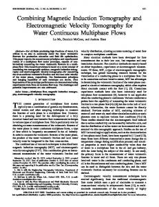
(9) As may be noted, the error is related to the number of test cases , and to values, which we call higher-order error terms, in turn related to and values. Thus, once the profile (determining the values) is decided, the expression depends on and on terms: , with deriving from the correct profile. According to (9), if , and conversely if . The latter case is of interest because is the technique actually applied by practitioners, and they want it to deliver a lower failure probability. Thus, the relation between the error and establishes the following bounds. • Given a fixed budget of test cases , the weighted error on the operational profile must be at least greater than for OP testing to be better than the Error-free case. Therefore, it may be even negative, but it must be not less than . • Given a maximum tolerable error, , a tester must execute at least test cases to obtain the same or better performance than the Error-free case, where is the value for which . Note that, for , (9) provides when . This happens only for . To further clarify, we report, in Fig. 1(a), a numerical example with plotted against the number of test cases , given a negative value (which is the worst case for the tester). In this example, the initial and values are randomly selected, and reported in Table I.6 The figure shows five different curves, each one with a different value of the error, obtained by varying values. When the curve is positive, OP testing performs better than Error-Free OP testing. The crucial value of the number of test cases, , for which this happens is the intersection with the -axis. Note that, as the error approaches 0, such a number decreases from 133 down to 17 (i.e., with being close to 0, a lower number of test cases is required for OP testing to perform better than Error-Free OP testing). After this critical value, the performance of OP testing is always better. With the number of test cases approaching infinity, the performance of OP testing gets closer to the performance of Error-Free OP testing (they both tend to deliver a failure probability equal to 0). Fig. 1(b) provides a more complete view of . Given a (maximum tolerable) error value, the solid line suggests the number of test cases, , to allocate in order to have . As the error approaches 0, fewer test cases are needed for OP testing to perform better than the Error-free case. Finally, one more value of interest is the value of for which the curves of Fig. 1(a) exhibit their maximum value, indicating the best performance of OP testing; let us denote it with T-MAX. In Fig. 1(b), the dotted line depicts the relation between and T-MAX; it suggests the number of test cases to perform to have 6Note that the summation is not equal to one because it includes only failure regions, not all the input values of .
414
IEEE TRANSACTIONS ON RELIABILITY, VOL. 62, NO. 2, JUNE 2013
Fig. 1. Numerical example of OP testing performance. (a) Number of test cases vs.
TABLE I EXAMPLE: INITIAL AND
the best performance under a given error, and conversely what is the expected error to achieve in order to not overcome a given budget T-MAX, and obtaining the best performance. T-MAX starts decreasing from 500 when the error is less than about 4.3E-5, and then decreases rapidly with the error approaching 0. As an example, consider that, when the error values are the same as in Fig. 1(a), namely 4.24E-5, 3.35E-5, 2.46E-5, 1.57E-5, 0.68E-5, the corresponding T-MAX values are 470, 364, 310, 276, 251. These T-MAX values represent the number of test cases to perform in order to have the best performance of OP testing with those errors. From (9), and from this example, it is clear that, although (6) indicates the probability of OP testing being better than the ideal Error-free case, it is not exhaustive. That probability varies according to the number of test cases, and the profile estimation error. Equation (9) makes it explicit, giving the conditions under which OP testing outperforms the Error-free case. V. OP-D TESTING This section presents the OP-D testing approach. The idea behind the strategy is to exploit the combination of specular techniques with the goal of addressing failure regions both with high and with low operational failure rates. The debug testing approach used in this work, called “anti-profile” debug testing, is defined in Section III-B. The objective is to adopt OP testing until its detection ability no longer yields satisfactory results, and then switching to debug testing to increase the number of detected failure regions. Reliability will increase only if regions found by debug testing will have a total operational occurrence probability greater than the ones potentially found by
; (b) weighted error
vs.
and vs. T-MAX.
VALUES
continuing with operational testing. This condition is evaluated probabilistically. Let us denote with the expected failure probability delivered by the OP-D technique after test cases. With being the detection rates of debug testing, and the detection rates of operational testing, the expected failure probability of OP-D is given by (10) This equation considers the probability of the failure region not being detected by operational testing during test cases, not being detected by debug testing during test cases, and occurring at runtime .7 There are two factors that affect the performance of this combination: the accuracy of the operational profile, and the number of test cases devoted to debugging and to operational testing (or, in other words, the testing time to switch from operational to debug testing). In the following, the comparison between OP-D and OP testing is performed accounting for them. A. Single Residual Failure Region Let us first consider the simple case in which operational testing has been carried out until failure regions have been found. The residual number of regions is one. Let us denote this subset of failure domain as , being . The question is whether changing to debug testing improves or worsens the final reliability as compared to continuing with operational testing. 7In the subsequent analysis, we consider the OP testing with error in lieu of error-free OP testing, without loss of generality.
COTRONEO et al.: COMBINING OPERATIONAL AND DEBUG TESTING FOR IMPROVING RELIABILITY
Given , the failure probability of OP testing after test cases can be written as . Thus, the difference between and is determined by the second term (cf. with (10)). Assuming that all the failure regions except one, denoted with , have been detected during operational test cases, the comparison is reduced to verify whether
(11) where represents the increase in the failure probability caused by the residual failure region . In other words, the combined approach gives better reliability only if . For , it can be thought that this probability is high to the extent that is high. Intuitively, if the residual region has not been detected by operational testing in test cases, and is high, this means that its value is likely low; as a consequence its value is high. But this is not deterministic; we need to evaluate the probability that such an event occurs. In particular, we have that . Let us define these events as follows. , without any prior information; , with . Thus, . By Bayes’ formula, we have . Let us evaluate this expression. Because is derived from , the event may be written, recalling (2), as . Being the distribution function of , and posing , we have . The event represents the failure region not being detected during operational testing, given that . The probability that this event occurs, , is intuitively greater than because it considers only the cases in which (the smaller the greater the probability that it will not be detected by operational testing). In other terms, we are taking into account the case in which is selected in a range [0,1] (i.e., the event ), against the case in which the value is selected in a range , with (i.e., the event ), being (typically much smaller). Let us denote with this , and second case; thus,
415
greater than 0.5. This probability depends exclusively on , and . Because , it approaches 1 as approaches infinity. From the previous expression, it derives that (and thus ) . This relation establishes a lower with probability bound for the probability of the OP-D strategy to be better than OP testing, and a “confidence” in this bound. The probability that OP-D is better than OP testing is higher than with a confidence of . , Consider one more point from (12): if then the value increases (and thus OP-D improves) as increases because, in such a case, the ratio is greater than 1. This relationship is true because, if operational testing is not able to find in test cases, with very high, it means that the value is very low, and thus is very high. Thus, while the confidence depends only on the profile, the value of depends also on the number of test cases assigned to operational testing, . In fact, putting together the previous two statements leads to assert that the probability of OP-D being better than OP increases with (or with decreasing) with confidence . The amount of increasing of unreliability is directly related to , i.e., to the residual failure region: the failure probability increase in is , whereas the increase in is . B. Multiple Residual Failure Regions Let us now consider the case in which the number of residual failure regions after operational testing is greater than 1, i.e., . In this case, the delivered reliability depends on which regions among the residual ones are found by anti-profile debug testing, as compared to the ones that are found by continuing with operational testing, and on the sum of their failure rates. After the first phase of operational testing, the additional contribution to the failure probability is for OP-D testing, and for OP testing. Similar to the previous case, two events are defined: is the event , and is the event that has not been detected during operational testing, with The probability that is (13) It is clear that the increase in the failure probability depends on . Recalling (12) in the previous section, the expression may be written as
(12) Let us evaluate the ratio mulation, we have
0.5, meaning the ratio
. With this for-
. This value is always greater than with probability
(14)
416
IEEE TRANSACTIONS ON RELIABILITY, VOL. 62, NO. 2, JUNE 2013
The expression is regulated by two parameters: by , or equivalently, , and by the pair , depending on the profile. may determine the probability of OP-D being better than OP: in particular, if the ratio is greater than 1, then the corresponding failure probability increases with , meaning that OP-D testing behaves better as increases. On the other hand, the and pair determines the confidence at which that ratio is greater than 1. In fact, if is high, the probability that it is greater than 1 approaches 1 because the are more probably lower than . However, the pair affects also the failure probability value, not only the confidence (suffice it to note that the term goes to 0 as increases). In other words, given a selected profile, the corresponding depend on the cardinality of the input domain, (cf. with (2)). In this sense, this parameter regulates the confidence of the information on which technique behaves better; the amount of failure probability is then also determined, other than by the profile, by how the test budget is distributed as . In the end, the parameter is completely under the control of the tester, but the profile may be not; thus, in the next section, an analysis considering the features of the profile is carried out so as to help the tester find the best settings.
is therefore related to total the number of test cases , to the number of test cases devoted to debug testing , as well as to the profile determining and values. We then have
where denotes a function of , the second term of (17). These expressions regulate the probability of OP-D testing being better than OP testing, depending on the weighted differences between and values. However, it should be noted that the variable is also related to the error ; changing values of affects also the difference . In particular,
C. Profile vs. Test Cases in OP-D Testing Let us consider
. It may be written as
(18) (15) Results of this expression depend on the differences between values and the corresponding values. Thus, we define, similarly to the variable, the weighted difference . Equation (15) may be written as
Considering that, for sion is , we rewrite (16) as
, and
Thus, (19) . with The relationship between and implies a relationship between the error , , and in (17). It is expressed by
(16) , the previous expres. Replacing (20)
(17)
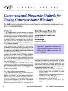
Thus, similarly to the case of OP Testing, the relation found helps establish values of and given a known error on the estimated profile, or to set the maximum tolerable error and the best for the OP-D testing to be better than OP testing, given a fixed budget of test cases . Fig. 2 shows the example of
COTRONEO et al.: COMBINING OPERATIONAL AND DEBUG TESTING FOR IMPROVING RELIABILITY
Fig. 2. Number of test cases for debug testing in the OP-D, with vs. , and .
,
Section IV, where the number of test cases is set, and the difference , as well as , is evaluated against the variation of . With , and with both positive and negative values, the best values for OP-D testing to be better than OP testing (or than Error-free OP testing) are those for which (or ) is maximum, i.e., around –180 (or –190). Note also that, as the error becomes larger, the range of good values gets reduced. After a given value, the curve decreases, indicating the better performance of OP testing; after that point, the decrease is rapid, and OP-D testing performs worse. Summarizing results of this section, and of Section IV, we may conclude that (6), and (14) provide the probability, respectively, i) of OP testing to be better or worse, from the reliability point of view, than the ideal Error-free OP testing, and ii) of OP-D testing to be better than OP testing. In comparison, (9) and (20) provide the relation between the weighted error on the profile and the number of test cases, and serve to set and to assure the best technique from a reliability perspective, given a maximum tolerable error on the profile. They may also be used to determine the range of tolerable error within which a technique is better than another, given a fixed testing budget. To have a complete picture, the impact of all the involved parameters is now evaluated by simulation. VI. SIMULATION The findings of the previous sections are checked through simulation, by randomly generating several operational profiles, and evaluating the performance of techniques with respect to the involved factors. A. Procedure The parameters considered in the simulation are the weighted error value , the number of test cases , the number of test cases devoted to debug testing in the OP-D approach , , the cardinality of the input domain , and the number of failure regions present in the software . Note that the weighted difference is proportional to . Thus, the corresponding scenario is not showed. These parameters of interest
417
determine a final set of four scenarios, described in the following. To carry out experiments, we implemented a procedure to accomplish the following steps. 1) Operational profile generation, by generating random numbers between 0 and 1 for each input, and then normalizing them. 2) Operational profile generation with error. 3) Debug testing profile generation, by (2). 4) Choice of the failing inputs by randomly picking numbers between 0 and for each experiment. 5) Given the limits of the parameter values to be varied in the experiment, the algorithm computes the expected failure probability of each approach. B. Experiment 1 The first scenario deals with operational profile characteristics. In this experiment, the operational profile error is varied to observe the performance of OP and OP-D in the presence of error. To evaluate the OP-D approach, three different configurations are set for : 15%, 45%, 75% of the total number of test cases . For this experiment, four different configurations are evaluated: the cardinality of the input domain is and then , the number of test cases is and then . In all the four configurations, the number of failure regions is . Note that the operational profile assumed to be correct is generated in each setting, and consequently the profiles affected by error are regenerated each time. For this experiment, 50 different profiles are generated in each configuration. A profile is generated by sampling random numbers between 0 and 1 for each input (i.e., times), and then by normalizing each number with respect to the sum of all the generated numbers, so that the input values add to 1. In Fig. 3, the dotted line represents the delivered failure probability resulting from Error-free OP testing. For each curve (i.e., the applied testing technique), each point in the graph represents the expected failure probability ( -axis), obtained by applying the corresponding technique, considering an operational profile with a given estimation error ( -axis). When such a value is lower than the value of the dotted line, it means that the technique performed better than Error-free OP testing; in these cases, the error on the profile estimation is in the conditions that we found analytically, and the observed performance is better than the ideal Error-free case. In particular, if the error is greater than for OP testing, it is more probable to pick failing inputs in the testing phase than in the operational phase, and the testing performance is good. In the same way, if , then OP-D testing outperforms OP testing, and possibly the Error-free OP testing as well. We observe results in the left part of the graphs, where , and in some cases . This condition of course happens more often when is positive for OP testing, and when is negative for OP-D testing. Thus, OP testing becomes better as the error increases, contrarily to the OP-D approach. The specular behavior between OP and OP-D testing is observed because, when the error is negative, values are on average lower than ones, and at the same time values are higher, making OP-D perform better.
418
Fig. 3. Experiment 1. (a)
IEEE TRANSACTIONS ON RELIABILITY, VOL. 62, NO. 2, JUNE 2013
,
; (b)
,
; (c)
Whereas, when the error is positive, values are on average higher than ones, and at the same time values are lower, making OP-D perform worse. In most of the experimental points in this example, the OP-D approach exhibited a lower failure probability. OP testing behaves better when the error becomes a sufficiently large positive value. As the error approaches 0, all the experimented techniques tend to have the same performance. One more point to highlight is that OP testing tends to have greater fluctuations than OP-D testing; combining techniques tends to limit the effect of the profile estimation error on the variation of results because, by addressing both high with operational testing, and low with debug testing, it balances the performance between cases with different . The technique that exhibits the most stable behavior is the OP-D 45%, namely the OP-D technique with of the total number of test cases . C. Experiment 2 Experiment 2 compares techniques with respect to the number of test cases . The delivered failure probability of each technique decreases with the increase of test cases, so the goal is to compare the decreasing behavior of each technique. , and then ; The fixed parameters are is either considering results of Experiment 1, the error . positive or negative; and
,
; (d)
,
.
Figs. 4(a)–4(d) show comparable trends. In particular, regardless of the weighted error , there is a number of test cases for which OP-D testing behaves better than the others; of course, as tends to infinite, all approaches go to 0. OP testing shows the worst performance; in the first scenario (Fig. 4(a)), it starts better than the others, but as the number of test cases increases it gets worse. In most cases, OP-D is better than OP testing, in the sense that it converges earlier to 0, employing fewer test case to obtain the best performance. In particular, OP-D with 45% of exhibits the best performance. In all the cases except the one in Fig. 4(c), it goes even better than the Error-free case. In the scenario of Fig. 4(c), 45% OP-D is still worse at ; but, by extrapolating the trend, we see it should converge earlier to 0 than Error-free OP testing. D. Experiment 3 In the previous experiment, we showed that the OP-D approach eventually behaves better than OP, with different convergence speed depending on the operational profile characteristics. This experiment investigates in more detail the impact of , i.e., of the proportion of test cases allocated to debug testing, with respect to operational testing, in the OP-D solution. Thus, as above, this instead of considering 3 percentage values of experiment allows varying from 0% of (which corresponds to the pure OP testing) up to 90% of . The fixed parameters are , , and is considered to be , either positive or negative.
COTRONEO et al.: COMBINING OPERATIONAL AND DEBUG TESTING FOR IMPROVING RELIABILITY
Fig. 4. Experiment 2. (a) positive, zoomed in
Fig. 5. Experiment 3. (a)
,
negative. (b)
,
positive. (c)
419
,
negative, zoomed in
. (d)
,
.
,
negative. (b)
,
positive.
The observed behavior shown in Fig. 5 is similar to a bathtub curve, as also showed by the example in Section V. The starting value 0 represents the OP testing. The failure probability decreases suddenly as increases, and outperforms the Errorfree OP testing (represented by the constant line) in a range, starting at about 10%–20% to 75%–85% of . Then, besides that value, OP-D performance gets worse. The best values for Fig. 5(b) are between about 320 and 520 out of 900 test cases, i.e., between 35% and 57% of ; while in Fig. 5(a), with negative , the interval is between 370, 41%, and about 600, 66%. In the case of the example in Fig. 2, the comparison between
OP-D and Error-free OP testing suggested a value between 170 and 190 out of 500 (i.e., between 34% and 38% of ) for the difference to be the maximum, confirming that the central part of the curve provides the best performance. In general, the differences in such percentages depend on the value of ; to compute the best given an , (20) must be used. E. Experiment 4 This experiment shows the variation of performance with re, with , and spect to the number of failure regions, then , also with . The performance, shown
420
IEEE TRANSACTIONS ON RELIABILITY, VOL. 62, NO. 2, JUNE 2013
Fig. 6. Experiment 4. (a)
. (b)
.
in Fig. 6, gets worse as the number of failure regions increases; the increasing for all the techniques is approximately linear. OP testing increases more rapidly than the others; the OP-D combination performs better also in this case. The behavior of OP-D 45% testing is confirmed to be the best also in this case. Overall, the conducted simulation suggests that the OP-D solution with performs better than the others. The experiments confirm this outcome with several parameter configurations: in Experiment 1, OP-D at 45% was evidently the most stable solution with respect to the error (it is almost constant); in Experiment 2 and Experiment 4, the OP-D at 45% had the lowest failure probability value in all the experimented cases; Experiment 3 showed that the lowest point in the bathtub curve is in the central part, thus close to 45%. VII. A CASE STUDY EXAMPLE The case study chosen for illustrative purpose is an application developed for the European Space Agency called Space. It is a program to provide the user interface for the configuration of an array of antennas, and it functions as an interpreter for an array definition language (ADL). Its purpose is to prepare a data file according to a predefined format, given the array antenna configuration described in ADL. If the input ADL file is correct, Space outputs an array data file containing a list of array elements, positions, and excitations; otherwise, it outputs an error message. The program consists of 9564 lines of C code (6218 executable), and has already been widely used in several previous studies on reliability analysis, evaluation, and software testing (e.g., in [9], [13]–[15]). The program is provided with 33 faulty versions containing faults discovered and recorded during testing and operation (the five additional faults found by [14] are not considered), and with 13585 test cases (each test case is an ADL file). The goal of our experiment is to compare OP-D testing against OP testing. OP-D at 45% has been chosen among the compared ones, as it showed the best performance previously. The following steps have been taken to perform the experiment.
1) We first assigned a value between 0 and 1 to each single available test case,8 representing the probability with which the considered input case would actually occur in operation. Each value is generated by a uniform random number generation in (0,1), and then normalized over the sum of all values so their sum is 1. The so-built distribution is assumed to represent the actual operational profile, denoted as . 2) Four further operational profiles have then been generated randomly in the same way, named , , , and . They are supposed to be the testing profiles for operational testing (meaning that test cases for OP testing are sampled from such profiles). From these profiles, we used (1) to create testing profiles for debug testing, named respectively , , , and . 3) After generating profiles, we run eight testing sessions: four with OP, and four with OP-D testing techniques. Specifically, we used 1500 out of the total number of test cases as the testing budget for each testing session; we first run the 1500 test cases with the OP testing method according to operational profiles , , , and . Then, we run OP-D testing, using the same profiles for the operational testing part (i.e., for 55% of the T=825 test cases picked up from profiles), followed by the corresponding debug testing profile (45% of the T=675 test cases from profiles). 4) During the testing sessions, failed runs have been detected by using the original Space program as the test oracle, i.e., applying test cases to the original and to the faulty Space program, revealing differences between the corresponding outputs. Because the same test case may trigger several faults, the fault removal has been performed as in [13], [18], assuming a one-to-one correspondence between failure and defect; when a software failure is observed, one and only one failure-causing defect is removed without new defects being introduced. Table II reports the number of the test case that exposed a failure, from which a (seeded) fault is removed. 8Test
cases are not partitioned into equivalence classes.
COTRONEO et al.: COMBINING OPERATIONAL AND DEBUG TESTING FOR IMPROVING RELIABILITY
421
TABLE II TOTAL DETECTED FAULTS AND FINAL RELIABILITY
5) After this phase, the reliability of the program with residual defects has been estimated by running the software under the real operational profile , by executing 2300 runs (without removing defects) selected according to the actual profile . Reliability is estimated as in [13], [16]: , with being the number of failed executions, and the number of total executions, selected according to . The final reliability is in the last row of Table II, which confirms the superiority of the OP-D approach as compared to OP testing, for the considered example. VIII. SUMMARY, AND FINDINGS In the previous sections, we examined operational testing by simulation, and via a case study; we attempted to address the issues hindering its adoption by practitioners. To get closer to the realistic application of this technique, several factors are included in the analysis, ranging from the number of test cases to the profile features. Most importantly, given that it is realistically difficult to avoid an error in estimating the operational profile when the technique is applied in practice, the impact of such an error on the result is formalized, and then evaluated. Software developers often distrust operational testing because they believe that a actual profile is not a meaningful concept. The introduction of the profile error measure and its relation with the number of test cases is essential to address the issue of inaccurate operational profile estimation. Besides the analysis of operational (OP) testing, the paper proposed a new approach to testing software with the goal of improving its reliability. The combination of operational testing with a debug testing technique, namely the anti-profile debug testing, is presented; and its performance is analyzed with respect to OP testing. The main findings of these analyses are the following.
• OP testing affected by error in the profile estimation is different from Error-free OP testing, as expected. But it may perform better than the error-free case. • The new conceived approach, OP-D testing, is probabilistically better than OP testing; numerically, and by simulation, it has been shown to behave better in most of cases. • It has been possible to establish the analytical conditions in which actual operational testing (namely, OP testing with error) is better than Error-free OP testing, and in which OP-D testing is better than OP testing, depending on the error on the profile, and on the parameters related to the number of test cases . • In general, the exact amount of test cases in the OP approach, and of operational or debug test case proportion in the OP-D approach must be decided by means of the analytical formulas from Sections IV and V, depending on the expected, or the tolerable, error on the profile, on the desired performance, and on the budget in terms of test cases. • By simulation, we found that the OP-D solution is better than OP testing in most of the tried settings, and that OP-D with 45% of the debug test cases is the best approach among those tried (15%, 45%, 75%); it is more robust to operational profile estimation error, and delivers always the least failure probability at the end of testing. Such results are a confirmation of analytical findings. • By simulation, OP-D testing shows a lower variability in the results than OP testing (and OP-D testing with 45% of shows the lowest one), probably because combining operational and debug test cases assures, in the average, to address always both failures with high occurrence frequency at operational time, and failures with low-occurrence frequency. Variability of performance is also regulated by the cardinality of the input domain (the larger it is, the more stable the results).
422
IEEE TRANSACTIONS ON RELIABILITY, VOL. 62, NO. 2, JUNE 2013
• Experimentally, the application to a case study confirmed the good results of 45% OP-D as compared to OP testing in terms of delivered reliability. However, care must be taken in generalizing the observed behavior. In fact, i) the number of trials (i.e., of testing sessions) is not sufficient to claim a statistically significant superiority, and ii) choosing a case study implies that results are not generalizable a priori, so different results may be observed applying the approach to software programs with different features, application targets, size, and complexity. Moreover, in general, it may not be true that each test failure deterministically causes one fault to be removed, and the perfect oracle assumption (i.e., all test failures are noticed) may not hold. The experiment must therefore be viewed more as an example to confirm both analytical and simulation results on a concrete case study rather than as a statistically valid comparison between the techniques generalizable to other programs. IX. CONCLUSION Evaluating the impact of software testing techniques on delivered reliability is not common. There are indeed difficulties in this evaluation, related to nature of these attributes. This difficulty explains also why reliability is rarely adopted as pilot criterion to drive verification activities, or to select testing techniques. Operational testing, in spite of the encountered difficulties and its limits, is still the technique generally considered as oriented toward reliability, in contrast to debug testing which aims to maximize the number of detected bugs. Starting from operational testing, from its advantages and shortcomings, the paper tries to address again the topic of reliability-driven testing, i.e., it tries to figure out how to conceive testing approaches oriented toward a reliability improvement objective. Besides the obtained results, it is important to remark that, different from the past, our aim has not been to claim the superiority of operational over debug testing (or the opposite), because, as several studies showed so far, it depends on the context (e.g., it depends on operational profile and testing profile characteristics, on the profile estimation error, and on the occurrence rate of each failure). Our attempt has been to act on the limits of operational testing for high-reliable demands, and combine debug and operational testing for getting high delivered reliability. The objective of the proposed OP-D technique is to improve reliability with respect to applying only operational testing, while uncovering, at the same time, as many bugs as possible, as pursued by debug-testing. From this perspective, we believe that the view of operational testing compared against debug testing may in some sense be overcome. The final goal of any quality assurance activity is to deliver a program not failing in operation, i.e., highly reliable. From an operational tester perspective, the program may also contain bugs, but these must not be activated at runtime. However, for assuring this goal, operational testing should work perfectly (under the oracle of exact estimate of operational profile). On the other hand, from a debug tester perspective, the same goal may be achieved by trying to expose failures and remove as many failure regions as possible. But not considering the actual occurrence frequency of failures at operational time
may bring very little reliability improvement. These two views seem counter to each other, but they aim at the same objective, and may be suitably combined in their respective advantages: trying to expose higher-occurrence failure regions, and trying to expose as many failure regions as possible. For sure, for ultra-reliable systems, testers need to do both; thus, combining them makes sense. We intend to pursue this combination, further promoting the concept and practice of reliability-driven testing. REFERENCES [1] A. Wood, Software Reliability Growth Models Tandem Computers Inc., Tech. Rep. 96.1, 1996. [2] V. Almering, M. Van Genuchten, G. Cloudt, and P. J. M. Sonnemans, “Using software reliability growth models in practice,” IEEE Software, vol. 24, no. 6, pp. 82–88, 2007. [3] E. N. Adams, “Optimizing preventive service of software products,” IBM J. Res. Develop., vol. 28, no. 1, pp. 2–14, 1984. [4] P. G. Frankl, R. G. Hamlet, B. Littlewood, and L. Strigini, “Evaluating testing methods by delivered reliability,” IEEE Trans. Software Eng., vol. 24, no. 8, pp. 586–601, 1998. [5] B. Beizer, “The Cleanroom process model: A critical examination,” IEEE Software, vol. 14, no. 2, pp. 14–16, 1997. [6] R. Chillarege, I. S. Bhandari, J. K. Chaar, M. J. Halliday, D. S. Moebus, B. K. Ray, and M. Y. Wong, “Orthogonal defect classification-a concept for in-process measurements,” IEEE Trans. Software Eng., vol. 18, no. 11, pp. 943–956, 1992. [7] B. Zachariah and R. N. Rattihalli, “Failure size proportional models and an analysis of failure detection abilities of software testing strategies,” IEEE Trans. Rel., vol. 56, no. 2, pp. 246–253, 2007. [8] J. D. Musa, “Operational profiles in software-reliability engineering,” IEEE Software, vol. 10, no. 2, pp. 14–32, 1993. [9] C. G. Bai, C. H. Jiang, and K. Y. Cai, “A reliability improvement predictive approach to software testing with bayesian method,” in Proc. Chinese Contr. Conf., 2010, pp. 6031–6036. [10] P. Frankl, D. Hamlet, B. Littlewood, and L. Strigini, “Choosing a testing method to deliver reliability,” in Proc. 19th Int. Conf. Software Eng., 1997, pp. 68–78. [11] K. Y. Cai, “Towards a conceptual framework of software run reliability modeling,” Inf. Sci.-Informat. Comput. Sci.: Int. J., vol. 126, no. 1–4, pp. 137–163, 2010. [12] K. S. Trivedi, Probability and Statistics With Reliability, Queuing and Computer Science Applications (2nd edition ed.). Chichester, U.K.: John Wiley and Sons Ltd., 2001. [13] A. N. Crespo, P. Matrella, and A. Pasquini, “Sensitivity of reliability growth models to operational profile errors,” in Proc. 7th Int. Symp. Software Rel.Eng., 1996, pp. 35–44. [14] G. Rothermel, R. H. Untch, C. Chu, and M. J. Harrold, “Prioritizing test cases for regression testing,” IEEE Trans. Software Eng., vol. 27, no. 10, pp. 929–948, 2001. [15] F. I. Vokolos and P. G. Frankl, “Empirical evaluation of the textual differencing regression testing technique,” in Proc. Int. Conf. Software Maintenance, 1998, pp. 44–53. [16] R. Pietrantuono, S. Russo, and K. S. Trivedi, “Software reliability and testing time allocation: An architecture-based approach,” IEEE Trans. Software Eng., vol. 36, no. 3, pp. 323–337, 2010. [17] K. Y. Cai, C. H. Jiang, H. Hu, and C. Bai, “An experimental study of adaptive testing for software reliability assessment,” J. Syst. Software, vol. 81, no. 8, pp. 1406–1429, 2008. [18] K. Y. Cai, D. B. Hu, C. Bai, H. Hu, and T. Jing, “Does software reliability growth behavior follow a non-homogeneous Poisson process,” Inf. Software Technol., vol. 50, no. 12, pp. 1232–1247, 2008. [19] E. Weyuker, “Comparing the effectiveness of testing techniques,” in Formal Methods and Testing, R. M. Hierons, J. P. Bowen, and M. Harman, Eds. : , 2008, vol. 4949, Lecture Notes In Computer Science, pp. 271–291. [20] J. W. Duran and S. C. Ntafos, “An evaluation of random testing,” IEEE Trans. Software Eng., vol. 10, no. 7, pp. 438–444, 1984. [21] D. Hamlet and R. Taylor, “Partition testing does not inspire confidence,” IEEE Trans. Software Eng., vol. 16, no. 12, pp. 1402–1411, 1990. [22] P. G. Frankl and E. J. Weyuker, “A formal analysis of the fault detecting ability of testing methods,” IEEE Trans. Software Eng., vol. 19, no. 3, pp. 202–213,1993.
COTRONEO et al.: COMBINING OPERATIONAL AND DEBUG TESTING FOR IMPROVING RELIABILITY
[23] D. Hamlet, “Are we testing for true reliability?,” IEEE Software, vol. 9, no. 4, pp. 21–27, 1992. [24] M. Chen, A. P. Mathur, and V. J. Rego, “Effect of testing techniques on software reliability estimates obtained using a time-domain model,” IEEE Trans. Rel., vol. 44, no. 1, pp. 97–103, Mar. 1995. [25] P. Frankl and Y. Deng, “Comparison of delivered reliability of branch, data flow and operational testing: A case study,” in Proc. Int. Conf. Software Testing Anal., 2000, pp. 124–134. [26] S. Poulding and J. A. Clark, “Efficient software verification: Statistical testing using automated search,” IEEE Trans. Software Eng., vol. 36, no. 6, pp. 763–777, 2010. [27] J. A. Whittaker and M. G. Thomason, “A Markov chain model for statistical software testing,” IEEE Trans. Software Eng., vol. 20, no. 10, 1994. [28] C. Kallepalli and J. Tian, “Measuring and modeling usage and reliability for statistical Web testing,” IEEE Trans. Software Eng., vol. 27, no. 11, pp. 1023–1036, 2001. [29] P. Thevenod-Fosse and H. Waeselynck, “An investigation of statistical software testing,” Software Testing, Verification Re., vol. 1, no. 2, pp. 5–26, 1991. [30] J. D. Musa, “Software-reliability-engineered testing,” Computer, vol. 29, no. 11, pp. 61–68, 1996. [31] H. D. Mills, M. Dyer, and R. C. Linger, “Cleanroom software engineering,” IEEE Software, vol. 4, no. 5, pp. 19–24, 1987. [32] R. W. Selby, V. R. Basili, and F. T. Baker, “Cleanroom software development: An empirical evaluation,” IEEE Trans. Software Eng., vol. 13, no. 9, pp. 1027–1037, 1987. [33] P. A. Currit, M. Dyer, and H. D. Mills, “Certifying the reliability of software,” IEEE Trans. Software Eng., vol. SE-12, no. 1, pp. 3–11, 1986. [34] R. H. Cobb and H. D. Mills, “Engineering software under statistical quality control,” IEEE Software, vol. 7, no. 6, pp. 44–54, 1990. [35] R. C. Linger and H. D. Mills, “A case study in cleanroom software engineering: The IBM Cobol structuring facility,” in Proc. Comput. Software Appl. Conf., 1988, pp. 10–17. [36] J. H. Poore et al., A Case Study Using Cleanroom With Box Structures ADL Software Eng. Technol. Tech. Rep. CDRL 1880, 1990. [37] , M. R. Lyu, Ed., Handbook of Software Reliability Engineering. : IEEE Computer Society Press and McGraw-Hill, 1996. [38] L. Strigini and B. Littlewood, Guidelines for Statistical Testing (Report No. PASCON/WO6-CCN2/TN12), 1997, ESA/ESTEC project PASCON. [39] L. Madani, C. Oriat, I. Parissis, J. Bouchet, and L. Nigay, “Synchronous testing of multimodal systems: An operational profile-based approach,” in Proc. 16th IEEE Int. Symp. Software Rel. Eng., 2005, pp. 325–334. [40] T. Y. Chen, F.-C. Kuo, and H. Liu, “Application of a failure driven test profile in random testing,” IEEE Trans. Rel., vol. 58, no. 1, pp. 179–192, 2009. [41] T. Y. Chen, F.-C. Kuo, and H. Liu, “Distributing test cases more evenly in adaptive random testing,” J. Syst. Software, vol. 81, no. 12, pp. 2146–2162, 2008. [42] K. Y. Cai, “Optimal software testing and adaptive software testing in the context of software cybernetics,” Inf. Software Technol., vol. 44, no. 14, pp. 841–855, 2002. [43] K. Y. Cai, B. Gu, H. Hu, and Y. C. Li, “Adaptive software testing with fixed-memory feedback,” J. Syst. Software, vol. 80, no. 8, pp. 1328–1348, 2007.
423
[44] K. Y. Cai, Y. C. Li, and K. Liu, “Optimal and adaptive testing for software reliability assessment,” Inf. Software Technol., vol. 46, no. 15, pp. 989–1000, 2004. [45] G. J. Myers, The Art of Software Testing. New York: Wiley, 1979. [46] C. Sarbu, A. Johansson, N. Suri, and N. Nagappan, “Profiling the operational behavior of OS device drivers,” in Proc. 19th IEEE Int. Sym. Software Rel. Eng., 2008, pp. 127–136. [47] C. Trammell, “Quantifying the reliability of software: Statistical testing based on a usage model,” in Proc. 2nd IEEE Int. Software Eng. Standards Symp., 1995, pp. 208–218. [48] M. Riebisch, I. Philippow, and M. Gotze, “UML-Based statistical test case generation,” Objects, Components, Architectures, Services, Appl. Netw. World, vol. 2591, pp. 394–411, 2003. [49] J. D. Musa, “Sensitivity of field failure intensity to operational profile errors,” in Proc. 5th Int. Symp. Software Rel. Eng., 1994, pp. 330–333. [50] O. J. Silva, A. N. Crespo, M. L. Chaim, and M. Jino, “Sensitivity of two coverage—Based software reliability models to variations in the operational profile,” in Proc. 4th Int. Conf. Secure Software Integr., Rel. Improvement, 2010, pp. 113–120. [51] M. H. Chen, A. P. Mathur, and e V. Rego, “A case study to investigate sensitivity of reliability estimates to errors in operational profile,” in Proc. 5th Int. Symp. Software Rel. Eng., 1994, pp. 276–281. [52] C. Y. Huang and M. R. Lyu, “Optimal testing resource allocation, and sensitivity analysis in software development,” IEEE Trans. Reliability, vol. 54, pp. 592–603, 2005.
Domenico Cotroneo received the Ph.D. in 2001 from the Department of Computer Science and System Engineering at the University of Naples “Federico II”. He is currently associate professor at the same university. His main interests include dependability assessment techniques, software fault injection, and field-based measurement techniques. Dr. Cotroneo has served as Program committee member in a number of scientific conferences on dependability topics, including DSN, EDCC, ISSRE, SRDS, and LADC; and he is involved in several national and European projects in the context of dependable systems.
Roberto Pietrantuono , Ph.D., is currently a post-doc at University of Naples “Federico II”, Italy. He received his Ph.D. degree (2009) in Computer and Automation Engineering from the same university. He collaborates with several companies of the Finmeccanica group, in the field of critical software system development. His research interests are in the area of software reliability engineering, particularly in software verification of critical systems, software testing, and software reliability analysis.
Stefano Russo is a Professor and the Deputy Head at the Department of Computer and Systems Engineering, Federico II University of Naples. He is the Chairman of the Curriculum in Computer Engineering, and Director of the “C. Savy” Laboratory of the National Inter-Universities Consortium for Informatics (CINI). His research interests are in the areas of distributed software engineering, middleware technologies, and dependable software systems. He coordinates the national project DOTS-LCCI on software dependability for critical infrastructures. He has (co-)authored more than 120 scientific papers.