Combining Parallel Coordinates with the Reorderable Matrix Harri Siirtola Information Visualization Research Group TAUCHI – Tampere Unit for Computer-Human Interaction Department of Computer and Information Sciences FIN-33014 University of Tampere
[email protected] +358-40-54-88700
Abstract There is evidence that the highlighting of the same data items in different views will improve the proficiency of knowledge acquisition tasks. Making the connection for the user will reduce the cognitive load of switching from one view to another and allows making observations that would not be possible from the two separate views. However, making the connection between conceptually different views might not be so straightforward if the view types are complex and different enough. This paper compares two conceptually different information visualization techniques called parallel coordinate plots and the Reorderable Matrix, and considers how the two representations could be combined. We report an experiment where the participants performed tasks with an application having a Reorderable Matrix and parallel coordinates views to the same data, with linking and without linking. It was found out that although the view linking initially slows the task performance, it will accelerate learning and it is well received by the users. Keywords – Information visualization, multiple views, view linking, the Reorderable Matrix, parallel coordinate plots.
1. Introduction One important class of problems that the information visualization research is addressing is the visualization of multidimensional data. A data set is considered multidimensional (or multivariate, or even hypervariate) when it has about five or more variables. For this kind of data, we do not have a standard presentation method. As a problem, the exploration of multidimensional data is common, and it is often characterized as the visual data mining process.
Statisticians – who are experts on multidimensional data – represent a multidimensional data set often as multiple scatter plots. The cross-tabulation approach is fine for pairwise observations, but relations that are more complex are hard to detect. Ideally, we would like to make observations on single data items, on subsets of data items, and on the overall data sets. It is obvious that a static representation of multidimensional data set cannot fulfill these requirements. One of the approaches to visualize information is to use tightly-coupled multiple views for presentation [1, 2, 3]. Among others, Schmid and Hinterberger [4] have considered combining conceptually different graphic displays for the visualization of multidimensional information. They have implemented a tool that has the following view types: a scatterplot matrix, a parallel coordinates plot, a permutation matrix, and an Andrew’s curve view. They also post a question “which method when” and they discuss the problem of connecting conceptually different graphic displays together. This paper considers in more detail one of the problems they pose: the linking of the permutation matrix and the parallel coordinate plot. This specific case is investigated to reveal issues and problems that are more general and applicable to other view linking problems. Figure 1 illustrates the problem. Suppose we have the same data set displayed in a parallel coordinate browser and as a permutation matrix. Now if we do an operation in one of the interfaces, what should happen in the other one? Even a simple selection in one of the interfaces does not necessarily have a natural interpretation in the other one, as we will see. In addition, these interfaces have considerably different means to support the human cognition struggling with complexity. This paper is structured as follows. We first consider the complexity as a phenomenon and the mechanisms that humans possess to deal with it. Then we present user interfaces for two techniques we are discussing, and present the problem of linking these conceptually different views
Figure 1. Two visualizations of the same data.
together. The final section before conclusions reports an experiment that was conducted to learn about the effects of view linking.
2. Complexity One broad characterization of the information visualization process is that it tries to make a complex setting easier to understand. In order to enhance this process, we need to understand the complexity as a phenomenon. In general, when we regard something as ‘complex’, it usually means that the ‘something’ has a large number of parts, or that the parts have non-simple relations, or both. A classic example of a complex ‘thing’ is the structure of any biological construction – the basic component is a cell, then we have tissues made out of cells, organs made out of tissues, and systems made out of organs. To support the understanding of this kind of constructions, we have developed certain strategies. The basic mechanisms for dealing with complexity are [5, 6]: • Decomposition • Abstraction
Another method for reducing the number of items we have to consider simultaneously is to chunk some of them together, or to form abstractions. Instead of dealing with a large number of properties, we concentrate on the essential ones and abstract the others away. This can also be regarded as a model-making approach – we construct an idealized model of the complex phenomenon and hide the unessential details. Classifying is the fundamental tool in organizing knowledge. If we have a good classification available, we can easily recognize the sameness and again reduce the number of items we have to consider simultaneously, by regarding classes of objects instead of individual items. The only problem in classification is that a good classification is difficult to come by. Another important concept related to the classifications comes from Herbert A. Simon’s work: it is the concept of a system being nearly decomposable. In general systems theory, a system can be divided into parts according to its intra-system and inter-system linkages: a sub-system is recognized if it has stronger internal linkages than external ones. Invariably this basis for decomposing is imperfect, and consequently the term ‘nearly decomposable’. In information visualization, the same situation arises when we try to decompose our data into subsets or classes: we have to consider tradeoffs between several possibilities, because the one ‘right’ answer does not usually exist. Finally, the formation of hierarchies is one of the techniques to master complexity. If we can identify substructures in a leveled fashion, we can again deal with a lower number of items at a time. Hierarchical structure is a natural one for humans, at least when we deal with something that is complex. Simon [5, p. 108] claims that we do not even understand complexity that does not take a hierarchical form. When we confront a new complex phenomenon for the first time, we try to disassemble it in a hierarchic fashion. A successful technique to visualize multi-dimensional information should support the presented human strategies for dealing with complexity.
• Classification
3. Parallel coordinates • Formation of hierarchies Decomposing means simply that instead of considering a large structure as a whole we divide it into manageable parts we can consider separately. The same principle has been an instrument in running nations and is now a fundamental tool in the creation of very large and complex systems built by software engineers. The effectiveness of decomposing is based on the channel capacity restriction in human cognition that can be circumvented by dividing a problem into smaller sub-problems.
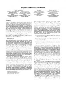
3.1. Visualization technique A parallel coordinate plot [7, 8] is a two-dimensional representation of an n-dimensional space. The idea is to display an n-dimensional data point as a set of connected line segments traversing through n parallel axes. For example, a point in a two-dimensional space is represented in the parallel coordinate plot as a line connecting the coordinate values on two axes, as can be seen in Figure 2.
x
y
y
(a,b) a x
There is a number of academic parallel coordinate browsers available, namely Ggobi [10], Visulab [4], XmdvTool [11], Mondrian [12], Parallel Coordinate Explorer [9], and some commercial ones, like Parallel Visual Explorer by IBM, and Parallax [13] from the creator of the parallel coordinates concept. This list is not exhaustive.
b
3.2. Tools for reducing complexity
Figure 2. A point (a, b) displayed in orthogonal space and as a parallel coordinate plot.
In a parallel coordinate plot the problem of adding more dimensions is handled simply by adding more parallel axes. In Figure 3 we have a view into a six-dimensional space that would be difficult to visualize by conventional means. The only limitation for the number of dimensions the parallel coordinate plot can represent is the size of the display area. It has been used in cases with over 100 variables.
Figure 3. Points in six-dimensional space as a parallel coordinate plot.
A parallel coordinate plot can be made interactive by implementing it as a computer application. Such an implementation can transform a static representation of a data set into a visual query tool. The following operations are common in such tools [4, 9]: • Selection of a single n-dimensional line, revealing the tuple of values • Brushing an axis, highlighting the lines traversing through a brushed area • Reordering, hiding and revealing the dimension axes • An axis manipulation operation, like the changing of minimum/maximum values, is also known as zooming. There are also some more sophisticated query operations available, but for the current discussion, the set above is sufficient.
Decomposing. In a parallel coordinate browser we can produce decompositions with two methods. In the first one, we can decompose the data set by brushing a sub-set of the lines. In this case the brushing is performed within a single view – the brushed object is either one of the dimensions or a set of lines, and the highlighted objects are the lines that were touched. The decomposition is between the highlighted and non-highlighted set of lines, thus facilitating the comparisons between sets or focusing on one of them. The second method is the manipulation of dimensions: we can show and hide axes, and in effect produce a projection of the data set. Therefore, the line brushing corresponds to row-wise decompositions, and the dimension manipulation performs a column-wise decomposition. Abstracting. The parallel coordinate plot is an abstraction itself, but we can produce even higher-level abstractions with it. A set of selected lines can be represented with a single line showing the mean and deviation of the lines as proposed in [9]. Classification. Besides the manual decomposition of the data set, the parallel coordinate browsers can also be used to find classifications. Inselberg has proposed a technique [14] based on hypersurfaces that can find classifications automatically. However, this method is not interactive in nature and does not solve the problem of dealing with nearly decomposable classifications. Formation of hierarchies. The formation of hierarchies is the only human complexity tool that the parallel coordinates visualization does not directly support. This is understandable, since the whole idea of parallel coordinates is to flatten a high-dimensional space into a planar representation. Very large data sets are challenging to parallel coordinate browsers, since the large number of overlapping lines will occlude part of the data. Fua et al. [15] have experimented with visual hierarchies to reduce the occlusion problem. One possible approach to building hierarchies with parallel coordinates browsers is to take advantage of the dimension zooming. In this technique, a selection on one axis defines the new minimum and maximum values for that dimension. As a result, some of the lines fall out from the parallel coordinate plot, and we have created a sub-plot for the data set. With this approach, it is possible to divide the original dataset into hierarchical subsets that can even be
overlapping.
4. The Reorderable Matrix 4.1. Visualization technique The Reorderable Matrix [16, 17, 18] is a straightforward graphical presentation of a so called ‘cases-by-variables’ table. A data table laid out in this way has objects in columns and properties of those objects in the rows. The idea is to represent the data values with graphical symbols that have a size relative to the data value. On each row, the smallest value is depicted with a zero-sized (or empty) symbol, and the largest value fills the available space. In Figure 4 we have a typical cases-by-variables table. The cases named with letters in Figure 4 are cars, and the variables are properties of those cars: the miles-per-gallon value, the engine cylinder count, and so on.
make new observations about the data. The difficulty in this process is that for even a small matrix the number of permutations is large. For example, the matrix in Figure 5 has 19! × 8! ≈ 4.9 × 10²¹ permutations. It is obvious that searching manually for the interesting patterns is a slow and a cumbersome effort. The original tools to manipulate the Reorderable Matrix were based on photocopying machines, paper strips, and objects reminding domino pieces. Today the Reorderable Matrix can be implemented as a computer application providing the following operations: • Moving a row/column to a new position • Sorting the matrix into ascending/descending order according to a row/column • Reorganizing methods: transposing, and variable promoting and demoting • Automatic permutation of the whole matrix
Figure 4. A part of a data table describing cars. The same data table is shown as a Reorderable Matrix in Figure 5. It is obvious that it is easier to do observations from the graphical representation than from the data table.
Figure 5. The cars data table as a Reorderable Matrix. The Reorderable Matrix is also known as a permutation matrix, and the reason for this is how one interacts with the matrix. A permutation matrix holds the same information in the crossings of rows and columns even if we permute the order of rows and columns of matrix. By permuting the matrix, we can produce different patterns, and potentially
Moving a single row or a column and the matrix threading operations according to a row or a column were available already in the manual implementations. Schmid and Hinterberger [4] also describe a transpose operation, where the rows and columns exchange places. However, this is in conflict with the original idea of the Reorderable Matrix. A more appropriate reorganization method that is based on the data table transformations is described by Bertin [17, p. 253] and Card et al. [19, p. 21]. In the cars example, we have 406 cases and eight variables: MPG, HP, DISPL, CYL, ORIGIN, ACCEL, WEIGHT, and YEAR. The ‘case’ in the data table is a CAR and the variables are characteristics of a CAR. A reasonable reorganization in this example would be, for example, to promote the variable YEAR to a case – other variables would become averages within a year, and the variable CAR would be a multi-valued property within a year. In this example, we would move from an 8 × 406 data table to a 12 × 8 data table, as seen in Figure 6, and lose information on individual cars, but gain better presentation for comparing years to each other. Other possible candidates for promoting would be variables ORIGIN to compare cars from different continents, and CYL for comparing cars with different engine types. The motivation to permute a Reorderable Matrix automatically is to find the interesting patterns from the set of all arrangements. As mentioned above, the size of the search space grows rapidly as the size of the matrix grows, and is large for even small matrices. The problem of finding desirable arrangements is known to be NP-hard [20], therefore a variety of approaches has been tried. A number of implementations of the Reorderable Matrix with automatic permutation is available, for example by the researchers from the Eindhoven University of Technology
Table 1. Complexity management
Decomposition Abstraction Classification Formation of hierarchies
Parallel coordinates +++ ++ + +
The Reorderable Matrix + +++ ++
Figure 6. The promotion of variable YEAR. Table 2. Interaction techniques [21-23], by Lohninger [24], by Rao and Card [25] and by Schmid and Hinterberger [4]. In all these implementations, the automatic permutation is too inefficient to be useful in an interactive tool. A recent proposal [26] is a technique that uses barycenter heuristics to find the rectangular areas from a matrix and is fast enough to be used interactively.
Selection Drill-down Brushing Reordering
Parallel coordinates +++ + +++ +
The Reorderable Matrix ++ + + +++
4.2. Tools for reducing complexity Decomposing and abstracting. The Reorderable Matrix as a technique relies on the rearrangement and does not provide direct support to decompose or to form higher abstractions. An elementary abstraction mechanism in some implementations is the support of locking the rows and columns in a rectangular area together. Such an area can be regarded as an abstraction. Classification. The Reorderable Matrix was initially designed for ‘graphical information processing’, where the finding and recognizing of similar groups in data is an important step. The permutation matrix is also tolerant enough to be used when the groups in data are only ‘nearly decomposable’, as they often are. Formation of hierarchies. The variable promotion and demotion mechanism can be seen as a hierarchic tool in the Reorderable Matrix technique. Although the hierarchy is predetermined by the nominal and interval scale variables, it does provide a hierarchical view of the data set.
5. Combining the techniques 5.1. Motivation The parallel coordinates plot and the Reorderable Matrix are complementary in many respects, and therefore good candidates to supplement each other. They have also qualities that are common to both, like the ability to display a whole data set in a single view. The following two tables summarize the tools for complexity management in these techniques and the variety of
interaction tools that the parallel coordinate visualizations and the Reorderable Matrix provide. Table 1 and Table 2 also reveal the task-types that these two techniques are appropriate to deal with. The parallel coordinates visualization is at its best when we are searching outliers and anomalies in the data, and it can be used to detect correlations between variables. The Reorderable Matrix suits best for looking groups or classes within the data. Although the summary tables are somewhat subjective in nature, they do support the claim that the parallel coordinates and the Reorderable Matrix complement each other in many ways. This is important, since combining two techniques with similar strengths would probably just make the software tool more complicated to use without providing any improvement in performance.
5.2. Linking the views Suppose we have a user interface where the same data set is displayed as a parallel coordinates plot and as a Reorderable Matrix. We consider performing an operation in one of the views, and discuss how that operation should be reflected in the linked view. Selecting a single data item. The selection of a single data item in a parallel coordinate browser means highlighting a single polyline that represents one data tuple. In a Reorderable Matrix view, a single data tuple is represented by a single column, a case. When both views are in their canonical form, the connection is simple: the selected data item is highlighted in both views. This situation is illustrated in Figure 7.
Figure 7. Selecting a single data item. The opposite situation – selecting a single data item from the Reorderable Matrix – is slightly different. ‘A single data item’ in a Reorderable Matrix is one property of a specific ‘case’, and its counterpart in a parallel coordinate plot is a point on an axis. In Figure 8 we have a single selection in a Reorderable Matrix (property #5 of case J) that is shown as a single highlighted point on axis #5 in a parallel coordinate plot. The connection is even more complicated if there is a variable promotion in the Reorderable Matrix view. Now, the columns of the matrix represent a set of cases, and the rows represent mean values for the corresponding sets. Selecting a column from the matrix view can be shown in the parallel coordinates view by selecting the set of corresponding lines. However, the opposite case, selecting a single polyline from the parallel coordinates view, is problematic – now the selected data tuple is classified into one of the columns. If we now highlight the column, we give the wrong message. Probably we could use different kind of highlighting to indicate the nature of the connection, but it is a potential source of confusion. Selecting a subset of data items. In both techniques, it is possible to select several data items at once. In a parallel coordinate browser, the selection is again a set of complete tuples. In a Reorderable Matrix, the concept of ‘selection’ is more general – we can select complete data tuples, as well as complete rows that represent a set of all values for a dimension. The most general selection is any rectangular area in a matrix, which depicts a subset of variables for a
subset of cases. In Figure 9 we have several selections in a Reorderable matrix, and they are indicated in the parallel coordinate browser. Selecting a row or a subset of a row in the Reorderable Matrix will produce a set of selected points on an axis in the parallel coordinate browser, as can be seen with row #1. A column-wise selection from the Reorderable Matrix will show as a set of connected line segments, as is shown in the selection (C-G, #3-#6). Selecting a dimension. Parallel coordinate browsers often implement a selection of a dimension as a means to supply an argument for the following command, which is often some modification of the attribute (visibility, limits, placement). In the Reorderable Matrix the selection of an axis corresponds to a selection of a complete row. Permutation of dimensions. In both techniques, it is possible to permute the dimensions or, essentially, move the dimensions in relation to each other. The dimension moving in a Reorderable Matrix view means simply dragging a row into a new position, and in a parallel coordinates plot it means the move of an axis. In Figure 7 we have a situation where the Reorderable Matrix has been sorted along a column and the order of axes has changed accordingly. Forming a classification. With both techniques, it is possible to produce and explore classifications of a data set. The parallel coordinates variant operates on a set of highlighted polylines, and outputs rules that distinguish the selected lines from the rest of the data set. As a linking problem, this is similar to the handling of selections. The classification procedures for the Reorderable Matrix
Figure 8. A single selection in a Reorderable Matrix.
Figure 9. A set of selections in a Reorderable Matrix.
divide the whole data set into subsets at once. This could be reflected in the parallel coordinates browser by highlighting the suggested subsets with different colors.
6. Empirical evaluation To test the effect of view linking in the case of the Reorderable Matrix and the parallel coordinate browser we performed the experiment described in this section. The experiment sought answer to the following questions: • How consistently do participants find the more ‘natural’ user interface for a certain task? Moreover, does the view linking help with this? • Is there a significant difference in performance between the two interfaces?
Table 3. Variables in the experiment. Variable Subject Group Link Answer T PC RM Time Sequence UI
Interpretation Identifies the participant The order of Link condition; either “TF” or “FT” Boolean variable; indicates the presence or absence of linking The radio button selection; 1-3 Task window time in seconds The time spent in parallel coordinate window; seconds The time spent in Reorderable Matrix window; seconds The overall task execution time; seconds The task position in sequence; 1–20 The user interface; “RM”, “PC”, or or “Both” if both used
• What are the users impressions on the view linking? The connection between views does not include all the features discussed in the previous section. The following subset of features was implemented: • Selecting a single case or subset of cases is highlighted in the other view. • Selecting any rectangular area from the Reorderable Matrix is also highlighted in the parallel coordinates view. • The row permutation of the Reorderable Matrix is linked to the axis order of the parallel coordinates browser and vice versa. Selection highlighting is not completely symmetric, because the current parallel coordinate browser does not support selection of line segments. This was not seen as a serious problem.
6.1. Subjects Twenty employees of our research unit volunteered to participate in the experiment without compensation. Six participants were women and fourteen men. The median age was 27 years with a range from 23 to 44 years. All participants were experienced computer users. The median of computer use was 15 years (range from 5 to 20 years) and the median daily computer use was 7 years (range 3 to 18 years). Some participants were familiar with the user interfaces used in the experiment, but none had seen the combined version.
6.2. Design Each participant performed 10 tasks with linked views and 10 tasks without linking. The order of blocks was balanced between participants and the order of tasks inside each block was randomized. The two task sets were isomorphic, but involved different cases and variables to prevent contamination. In effect, each participant performed two similar sets of ten tasks in random order. The program logged values for the variables shown in Table 3. The variable Time is the overall time of a task execution and is slightly more than the sum of variables T, PC, and RM.
6.3. Materials and apparatus The program for this experiment was constructed by combining two prior prototypes and removing the features that were not essential. The program was also instrumented to collect the time spent in each view and to record the answer that was given. A third view that presented the task and collected the answer was added. There was also a button to request the next task on the task window. The experiment was carried out on a desktop computer with a large enough display to fit all three views without overlap. The machine was also fast enough to respond instantaneously to user actions with this relatively complex Java application. To ensure sufficient screen refresh rate the display routines were implemented with OpenGL using the GL4Java library. The data set that was used in the test is artificially generated, near-random data. Some dependencies were fabricated in the random data to make the tasks more interesting.
Table 4. The task types. Task type The case C1 has a large value on variables V1 , V 2 , . . . , V n . How do the values of cases C2 , C3 , .., Cm compare to these? Cases, which have a small/large value on V1 and a small/large value on variable V2 , have the following kind of value on V3 . Cases C1 , C3 , .., Cn resemble each other. Variables V1 and V2 behave similarly. There exists cases which have all the variable values on the low/high end of the corresponding scale. A case, which has the smallest/largest value on variable V1 , also has the smallest/largest value on variable V2 .
“Natural” interface RM
Subjectiveness
PC
What is considered small or large.
RM RM PC
PC RM
None.
Threshold for similarity. Threshold for similarity. None.
questions about the interfaces, if the need arose. After the test the subject completed a feedback questionnaire and had a chance to comment on the experiment and ask questions. The exercise phase took from 10 to 15 minutes and the actual test from 30 to 54 minutes (median 37 minutes). The participants were instructed to do the tasks as quickly as possible, but to strive for the correct answers. They were also encouraged to use the two data views as they saw appropriate.
6.5. Results Task execution time. The grand mean of the variable Time for solving a task is 58 seconds. The comparison between groups solving tasks with linked views (Link = True) and with non-linked views (Link = False) can be seen in Figure 10. The mean for the condition “Link = False” is 52 seconds and for the condition “Link = True” the mean is 63 seconds. The t-test for the true difference of means is significant, suggesting that the means are different (p < .001, df = 370, two-sample t-test without assuming equal variances).
None
The cases were named with letters from the beginning of the alphabet and the variables were named with row numbers. The size of the data set was 23 cases ×18 variables = 414 data items. Using this data rules out the effect of domain knowledge. The task types are summarized in Table 4. The answer to a task was given by selecting one of three radio buttons on the task window and pressing a button labeled “Next” (in Finnish). The labels on the radio buttons changed appropriately for each task. For assertion tasks the labels were “True”, “False”, and “Unknown”. In comparative tasks the labels were accordingly “Higher”, “Lower”, and “No connection”.
6.4. Procedure The procedure can be divided into four parts. At the beginning participants filled a demographics questionnaire and were explained the nature of the test. Then the experiment supervisor demonstrated the two user interfaces and the subject tried out the features while they were explained. During the test the supervisor only observed and answered
Figure 10. The difference in means between conditions “Link = True” and “Link = False”. A learning effect is expected in this kind of repeatedmeasurement experiment. Figure 11 shows the distribution of task execution times in the sequence the tasks were performed. The average time to solve a task is clearly declining from the left to the right. This phenomena was counter-
balanced with the block design and with the task order randomization.
Figure 12. Interaction between variables Link and Group. Figure 11. Boxplot of the variable Time versus the task sequence. Table 5. Matching the task and the UI The analysis of variance was performed for the following nested model: • Time, the dependent variable;
“Wrong” Answer “Right” Answer
“Wrong” UI 21 78
“Right” UI 40 261
• Subject, the random effect; • Group, between-subjects factor; • Task and Link, two within-subjects fixed effects. The analysis confirmed that the effect of Link is significant, F1,19 = 25.96, p < .001. There is also a significant interaction between variables Link and Group, F1,19 = 28.51, p < .001, which is illustrated in Figure 12. There are two conditions defined by the Group. In the “TF” condition the views are linked in the first 10 trials (Link = True) and un-linked in the last 10 trials (Link = False), and the “FT” is the other way round. The interpretation for the interaction effect is that participants were faster on the second sequence of 10 trials than on the first sequence, as expected. However, they improved substantially more when they did the ”Link = True” condition first compared to when they did the ”Link = False” condition first. Task correctness. The median error rate for solving tasks was 2 out of 20. In the worst case there were 10 errors and in the best there were none. There was no statistically
significant difference between groups “Link = False” and “Link = True”. UI Selection. By inspecting the log file it is possible to compare the user interface that participants used to the interface that was assumed right for a task. It seems that the view linking does not have statistically significant effect on the selection of “right” user interface for a task. As seen in Table 5, the users would benefit from such guidance. The “wrong” and “right” are in quotation marks here, because there is a certain amount of subjective preference in the matching of task and user interface as well as in the definition of a correct answer. Another aspect of the UI selection is the distribution between choices. Of the 400 trials, 242 were performed with the Reorderable Matrix, 90 with the parallel coordinates browser, and 68 with both interfaces. This is the distribution for the top window position – it is of course possible to “use” a non-active window just by looking at it. Questionnaire. The questionnaire after the test contained eight propositions and participants were requested to comment them with six-step scale: “disagree completely”
– “disagree” – “disagree partly” – “agree partly” – “agree” – “agree completely”. In the following list three of the propositions have been reversed for easier interpretation. The value 1 corresponds to “disagree completely”. P1: “It is easy to choose the right view for a task.”
P2: “The view linking makes it easier to solve tasks.”
P3: “The Reorderable Matrix is easy to learn.”
P4:“The view linking helps in finding the right user interface for a task.”
P5: “The view linking improves task execution time.”
P6: “The view linking in the case of these two techniques is useful.”
P7: “The parallel coordinate browser is easy to learn.”
P8: “The Reorderable Matrix is easier to use than the parallel coordinate browser.”
6.6. Discussion Efficiency. The overall difference in mean of task execution time between linked and non-linked views was about 15% in favor of non-linked views. However, as Figure 12 shows, although the linked views are slower in both task sets, the learning effect is bigger in the group that begun with the linked views. They learned more about the tools during the first set and were in the better position to solve tasks without linking. It is also understandable that the linked views are initially slower: the user will glance the other view occasionally to see how the data appears in that view. The other aspect in efficiency is how accurate results we
can achieve. The error rate was almost identical for the two conditions, suggesting that the linking does not have effect on it. It is also apparent that there are answers that were misclassified because of the subjective differences in the concepts of “small”, “large”, or “similar”. This type of error does not affect the accuracy of task execution times, because usually the participants did the right thing to solve the task, but judged the fore mentioned concepts differently than the task designer. Subjective satisfaction. The propositions P2 and P6 clearly indicate that the participants found the view linking useful. Especially the group that did the view linking condition first missed the feature in their second set. Several subjects mentioned this either during the second set or in the post-experiment discussion. There was no clear preference over the two user interfaces, as the propositions P3, P7, and P8 indicate. The Reorderable Matrix was found slightly easier to use. Many of the participants favored a working style where they used the Reorderable Matrix as the input and confirmed their observations by checking the parallel coordinates view. The participants also believe that the view linking makes it easier to find the right user interface for a task, and makes it more efficient to perform them, as can be seen in the results of propositions P4 and P5.
7. Conclusions The motivation of linking conceptually different graphic displays together is in the fact that the different kinds of displays enable us to see different things from our data. The linking between views that show where in each view the current data item is will also reduce the cognitive load when we switch between the views. We have presented issues regarding the problem of combining conceptually different graphic displays. A specific case of linking the parallel coordinates plot and the permutation matrix was analyzed as an example where the conceptual differences are substantial. The results suggest that there are benefits in the linking of conceptually different views, even if they are complex and conceptually far apart. In the empirical study, the group that used the view-linked interface in the first set of trials performed clearly better in the end than the other group. This suggests that the view linking accelerates the learning of a complex user interface. It was also apparent that the users really like the idea of view linking and are willing to make use of it.
Acknowledgements This work was supported by the Academy of Finland (project number 178099) and by the TISE graduate school.
References [1] M. Baldonado, A. Woodruff, and A. Kuchinsky, ”Guidelines for using multiple views in information visualization,” ACM Advanced Visual Interfaces ‘00, 2000.
[15] Y.-H. Fua, M. O. Ward, and E. A. Rundensteiner, ”Hierarchical Parallel Coordinates for Exploration of Large Datasets,” IEEE Conference on Visualization ’99, San Francisco, CA, 1999. [16] J. Bertin, Semiology of graphics. Madison, Wis.: University of Wisconsin Press, 1983.
[2] C. North, ”Multiple Views and Tight Coupling in Visualization: A Language, Taxonomy, and System,” The 2001 International Conference on Imaging Science, Systems, and Technology (CISST’2001), Monte Carlo Resort, Las Vegas, Nevada, 2001.
[17] J. Bertin, Graphics and graphic informationprocessing. Berlin ; New York: de Gruyter, 1981.
[3] J. Roberts, ”On Encouraging Multiple Views for Visualization,” IV’98 - Proceedings International Conference on Information Visualization, London, 1998.
[19] S. K. Card, J. D. Mackinlay, and B. Shneiderman, Readings in information visualization : using vision to think. San Francisco, Calif.: Morgan Kaufmann Publishers, 1999.
[4] C. Schmid and H. Hinterberger, ”Comparative Multivariate Visualization Across Conceptually Different Graphic Displays,” SSDBM ’94, 1994. [5] H. A. Simon, The Sciences of the Artificial, 1st ed: The MIT Press, 1969. [6] G. Booch, Object-Oriented Design with Applications, The Benjamin-Cummings Publishing Company, 1991.
[18] J. Bertin, ”Matrix theory of graphics,” in Information Design Journal, vol. 10, 2001, pp. 5-19.
[20] H. Siirtola and E. M¨akinen, ”The barycenter heuristic and the Reorderable Matrix,” manuscript, submitted, 2003. [21] R. Daru and W. Adams, T.C.F, ”Interactive graphic heuristic procedure,” in Computer Applications in Production and Engineering, F. Kimura and A. Rolstadas, Eds.: Elsevier Science Publishers, Amsterdam, 1989, pp. 783-?807.
[7] A. Inselberg, ”Visualization and data mining of highdimensional data,” Chemometrics and Intelligent Laboratory Systems, vol. 60, pp. 147–159, 2002.
[22] H. P. S. Snijder, ”The use of genetic algorithms in spatial optimisation problems,” DDSS’94, 1994.
[8] A. Inselberg, ”Don’t panic ... just do it in parallel!,” Computational Statistics, vol. 14, pp. 53–77, 1999.
[23] M. H. Veenendaal, ”Subjective orderliness versus mathematically defined order in graphical data matrices,” DDSS’94, 1994.
[9] H. Siirtola, ”Direct Manipulation of Parallel Coordinates,” Information Visualization IV’2000, London, England, 2000.
[24] H. Lohninger, ”Multivariate exploratory data analysis by means of INSPECT,” Software Development in Chemistry, vol. 9, pp. 91-98, 1995.
[10] D. Swayne, D. Temple, A. Buja, and D. Cook, ”Ggobi: Xgobi redesigned and extended.” Proceedings of the 33th Symposium on the Interface: Computing Science and Statistics, 2001.
[25] R. Rao and S. Card, ”The Table Lens: merging graphical and symbolic representations in an interactive Focus+Context visualization for tabular data,” CHI’94, 1994.
[11] M. O. Ward, ”Creating And Manipulating NDimensional Brushes,” 1997.
[26] H. Siirtola and E. M¨akinen, ”Constructing and reconstructing the Reorderable Matrix,” manuscript, 2003.
[12] M. Theus, ”Interactive Data Visualization using Mondrian,” Journal of Statistical Software, vol. 7, 2002. [13] A. Inselberg, ”Parallax: Software for Multidimensional Visualization and Automatic Classification,” 2003. [14] A. Inselberg, ”Automated Knowledge Discovery Using Parallel Coordinates,” Data Viz II Workshop, George Mason University, Fairfax County, VA, 2001.