Combining Particle Filters and Consistency-based ... - CiteSeerX
Recommend Documents
using efficient Monte Carlo approximation of the gradients. Thereby, our ..... 3.3 Monte Carlo gradient estimation ..... [9] V. Verma, J. Langford, and R. Simmons.
real time applications of particle filters, however, sensor information arrives at a ... situations is to update the particle filter as often as possible and to discard ...
Filters for Tracking Closely Spaced Targets in Clutter. Murat Samil Aslan ... algorithms, such as Joint Probabilistic Data Association. (JPDA) [2], [6] and its ...
performance can be achieved with significant reduction in computational costs. Keywords: Maneuvering target tracking, interacting multiple model, particle filter.
1. Bayesian Filtering: From Kalman Filters to. Particle Filters, and Beyond ... V-G Monte Carlo Sampling Approximation . . . . . . . . . ... V-G.1 Importance Sampling .
Apr 11, 2005 - Why should you be interested in particle filters? Because, like Kalman filters, they're a great way to track the state of a dynamic system for which ...
*University of Alcalá, Department of Electronics, Alcalá, Spain. ..... Conference on Generative Systems in the Electronic Arts, Melbourne. (Australia), 2005.
2University of Washington, Dept. of Electrical Engineering, Seattle, WA. 1 Introduction ..... maximum likelihood trainin
Email: [email protected]. Abstract .... 1: a) Pioneer robot used throughout the experiments. b)-d) Map of an office environment along with a series of ...
marginal likelihoods in hidden Markov models. Amongst a broad ... an asymptotic-in-time variance growth rate criterion. The sampling .... n ) form an XN -valued time-inhomogeneous. Markov chain. ...... Bernoulli 6 323â338. [5] Bucklew, J. A. ...
and Mayne (1969) had proposed much earlier to use Monte Carlo methods, but the idea of re- sampling ...... Stochastic Modelling for Systems Biology, 2nd ed.
Deformable models, Similarity measure, Image retrieval. 1. INTRODUCTION ... Establishing similarity/matching between an input shape and the shapes ..... technique on very diverse 2D shape databases, allows, according to results ob- tained in ... segm
videos of power cables installed almost 30 years go (i.e. they cannot be easily discriminated from ... and the orientation) of subsea elongated structures such.
all compliant motion tasks involving polyhedral objects with a known geometry .... tinuous state parameters, that get their precise meaning only in the context of a ...
target in the search domain, Î. The location of the target, θ â Î â Rnθ , is ... p0(θ), is provided, using any information available a priori. The state of the ith ...
In this work, we present some examples of applications of the so-called. Rao-Blackwellised Particle Filter (RBPF). RBPFs are an extension to Particle Filters ...
tively generate a second matrix characterizing global constraints. The update rule .... L â Gt (â=element-wise multiplication) is generated as an element-wise ...
rithm is based on the particle filter, and we demonstrate it on a few simulation examples. 1 INTRODUCTION. The field of positioning in wireless networks is both.
ideas further and describe the role of MCMC resampling, as proposed by ... Finally, we present a generalisation of our own in which MCMC resampling.
scattering from particles, to image gas pressure, velocity and temperature by molecular Rayleigh scattering, and to measure electron temperature and electron ...
William Ng, James P. Reilly and Thia Kirubarajan [email protected]; ... arrival (TOAs) and the source amplitudes respectively of K. (assumed known) ...
The advantages of a particle filter for this particular application is that it ... The objective of map-matching is to recursively estimate position of the vehicle from a ...
AbstractâThe particle filtering technique with multiple cues such as colour, texture and edges as observation features is a powerful technique for tracking ...
Combining Particle Filters and Consistency-based ... - CiteSeerX
Approaches for Monitoring and Diagnosis of Stochastic. Hybrid Systems ...... [11] E. Wan and R. van der Merwe, 'The unscented kalman filter for non-.
Combining Particle Filters and Consistency-based Approaches for Monitoring and Diagnosis of Stochastic Hybrid Systems Sriram Narasimhan1 and Richard Dearden and Emmanuel Benazera 2 Abstract. Fault detection and isolation are critical tasks to ensure correct operation of systems. When we consider stochastic hybrid systems, diagnosis algorithms need to track both the discrete mode and the continuous state of the system in the presence of noise. Deterministic techniques like Livingstone cannot deal with the stochasticity in the system and models. Conversely Bayesian belief update techniques such as particle filters may require many computational resources to get a good approximation of the true belief state. In this paper we propose a fault detection and isolation architecture for stochastic hybrid systems that combines look-ahead RaoBlackwellized Particle Filters (RBPF) with the Livingstone 3 (L3) diagnosis engine. In this approach RBPF is used to track the nominal behavior, a novel n-step prediction scheme is used for fault detection and L3 is used to generate a set of candidates that are consistent with the discrepant observations which then continue to be tracked by the RBPF scheme.
1
Introduction
NASA’s vision for the twenty first century includes robotic exploration of deep space and human-robotic exploration of Mars and the moon. Safety is a major priority for all these efforts, for manned as well as unmanned missions. One key component for autonomous operation of such systems while ensuring safety is fault detection and isolation. For safety-critical systems, fast and efficient fault detection and isolation techniques are necessary in order to maintain a high degree of availability, reliability, and operational safety [10]. These systems tend to be hybrid in nature (a mix of discrete and continuous dynamics), hence both the discrete mode and continuous state of the system need to be tracked. In addition the systems and any models of the system are stochastic due to operation in uncertain environments and the presence of sensor and process noise. As a result diagnosis algorithms for such systems also need to be stochastic in nature. Bayesian belief update approaches to stochastic hybrid system diagnosis try to maintain an approximation of the true belief state either by sampling [5, 3] or by maintaining limited trajectories [4]. In order to deal with the continuous dynamics, the problem is broken up into a discrete mode estimation coupled with continuous state estimation. Typically Kalman filters are used to track continuous state and the estimated state is used as the observation function to update weights of particles or probabilities of trajectories. In these approaches the 1 2
fault is diagnosed by ensuring particles enter the true fault mode and then the observation function would keep increasing the weight of these particles. If there are a large number of fault modes then this requires a lot of computational resources since particles need to be put in all fault modes to make sure no fault is missed. On the other hand consistency-based approaches like Livingstone [12, 6] hand use structural and behavioral models (as opposed to transition models) to diagnose the faults. The system is modeled in abstracted form and the observations are also converted to this form (”monitors” for Livingstone). When the predictions from the model are not consistent with the observations, then the discrepancies are used to identify conflicts which are then used to identify possible fault candidates. These candidates can be tracked by comparing the predictions under these fault conditions against the observations. In this approach, rather than blindly guessing the faults, the constraints in the model are used to limit the candidates to be considered. However these approaches tend to be deterministic in nature (in some cases prior probabilities are used) and hence cannot deal with uncertain transitions and noise in the sensors and system. In this paper, we combine these two approaches in an effort to reduce the computational complexity associated with probabilistic approaches while extending Livingstone-like approaches to handle stochasticity. Our approach combines the look-ahead RaoBlackwellized Particle Filter (RBPF) [2, 5] and Livingstone 3 (L3) systems to provide a diagnosis architecture for stochastic hybrid systems. Section 2 describes the RBPF and L3 algorithms and also describes the unified modeling framework used by both diagnostic systems. In Section 3 we present the combined architecture and explain the different components of this architecture: the nominal observer, the fault detector, the fault observer and the candidate generator.
2 2.1
Preliminaries The Look-Ahead Rao-Blackwellized Particle Filter (RBPF)
The look-ahead Rao-Blackwellized particle filter [2] is detailed in Algorithm 1. It differs from the standard particle filter in two important respects. First, it maintains sufficient statistics (in the form of Gaussian means and covariances) for the continuous part of the system state. Thus each particle (sample) can be thought of as consisting of a sampled discrete mode plus a Kalman filter that represents a distribution over the continuous value the system could have in that mode. Secondly, the algorithm employs look-ahead to ensure that low-probability states are properly accounted for. While a standard particle filter samples new states from the transition prior distribution
(i)
P (Zt |zt−1 ) (the Monte Carlo step in a standard particle filter), lookahead allows us to incorporate the new observation to compute the (i) posterior distribution P (Zt |zt−1 , yt ) over states the sample could end up in, and sample directly from that. The look-ahead RBPF algorithm operates as follows. Assuming (i) that we use N samples, first the discrete mode z0 for each of the N is sampled from the given prior distribution Z0 over the modes (i) (i) (Step 1 in Algorithm 1). The mean µ0 and covariance Σ0 for the initial continuous state for each particle is also assumed to be given. At each time step three computations are performed which form the core of look-ahead RBPF. First, a look-ahead is performed for each sample. All successor modes for the sample are enumerated and the continuous state in each of these modes at the next time step is computed using a Kalman filter. The observation is then used to compute [ the posterior probability P ost(i, m) of the sample transitioning to the successor mode. The weight of the particle is re-calculated as the sum of these posterior probabilities. Secondly (Step 7), the particles are resampled as in the regular particle filter algorithm based on their weights. Thirdly (Steps 9 and 10), a new mode for each new particle is sampled from the posterior distribution computed in Step 5, and the mean and covariance are set to those computed for that mode by the Kalman filter in Step 4. Note that while look-ahead RBPF is limited to linear-Gaussian models by the use of a Kalman filter in Step 4, there is no reason why the Gaussian particle filter (GPF) [5] could not be used, allowing non-linear models to be tracked using the same algorithm. However, the use of an unscented Kalman filter [11] in the GPF algorithm complicates the discussion of our fault detection algorithm in Section 3.2 below.
1: Initialization: for N particles pi , i = 1, · · · , N , sample discrete (i)
(i)
(i)
modes z0 , from the prior P (Z0 ) and set µ0 and Σ0 to the (i) prior mean and covariance in state z0 . t = 1. (i) (i) (i) (i) 2: for all p = (zt−1 , µt−1 , Σt−1 ) do (i) 3: for each possible successor mode m ∈ succ(zt−1 ) do 4: Perform a Kalman update using parameters from mode m: (i,m)
(i,m)
(ˆ yt|t−1 , Sˆt
(i,m)
,µ ˆt
(i,m)
ˆt ,Σ
) (i)
(i)
← KF (µt−1 , Σt−1 , yt , θ(m)) 5:
Compute posterior probability of mode m as (i) [ P ost(i, m) ← P (m | zt−1 , yt ) (i)
(i,m)
(i,m)
= P (m | zt−1 )N (yt ; yt|t−1 , St|t−1 , yt ) 6:
Compute the weight of particle pˆ(i) : X (i) [ P ost(i, m) wt ← (i)
m∈succ(zt−1 ) (k)
7: Resample N new samples p(i) where: P (p(i) = p(k) ) ∝ wt . 8: for all p(i) do (i) 9: Sample a new mode m ∼ P (Zt | zt−1 , yt ) 10:
(i)
(i)
(i,m)
Set zt ← m, µt ← µt
(i)
(i,m)
and Σt ← Σt
.
Algorithm 1: The look-ahead RBPF algorithm
Observations & Commands
Transition System Model
Candidates
Constraints/Assumptions
Candidate Manager
Constraint Systems
Conflicts
Figure 1. Livingstone 3 Diagnostic Architecture
2.2
Livingstone 3 (L3)
The L3 diagnosis architecture ([9]) is illustrated in Figure 1. It consists of three main components. The system model stores the model of the system and is responsible for tracking the modes of operation of the different components and determining the constraints that are valid at any point in time. The constraint system serves the role of tracking the overall system behavior using constraint programming techniques. It receives constraints from the System Model indicative of the current configuration of the system and propagates these constraints to try to assign consistent values to variables in the system. When inconsistencies are seen (observations are different from propagated values for corresponding components), the candidate manager is responsible for using the conflicts generated as a result of these inconsistencies to generate candidates that resolve all the conflicts and that can possibly explain all of the inconsistencies. Algorithm 2 details the L3 approach. Each candidate ci is represented as a triple (F i ,(zt , st ),Et ) where F i is the set of fault transitions ((f1 , t1 ), . . . , (fj , tj )) that are hypothesized to have occurred (with their time of occurrence), zt is the discrete mode of the system and st is the state of the system at time t (current time) under the fault conditions and Et is the explanation graph tracing back from values of variables at time t to values of variables at time t − LT where L is some truncation limit applied to limit how far back we are willing to go in order to generate candidates. st includes all variables that have memory i.e., variables v whose values at time t, vt depend on their values at time t − 1, vt−1 . These may include continuous state variables x if the quantitative and continuous constraints are included in the Livingstone 3 models. Initially we only have the empty/null candidate in our candidate set C indicating our belief about no fault in the system. The initial discrete mode z0 and the initial state s0 are used as initial mode and state for the empty candidate. At this point the explanation graph for the empty candidate has only the variables from the current time step and no edges. At each time step t, we compute the new system discrete mode zt and instantiate the constraints q(zt ) into a constraint store Q for this mode. Note that the mode and constraints are actually composed from the modes and constraints for each component rather then pre-enumeration for all system modes. The state st is computed from st−1 (incorporating any transition conditions imposed by transition from zt−1 to zt ). We add edges st−1 → st and zt−1 → zt in the explanation graph. In addition if zt−1 to zt was a transition based on some decision function over internal variables (autonomous transition) we add edges from all st−1 involved in the decision function to zt . Finally we remove all
variables at time t−LT −1 (including st−LT −1 and zt−LT −1 ) from the explanation graph. The sensed input values ut = U are added as constraints q(ut ). The resulting set of constraints (constraint store) Q are propagated to infer values for other variables including the output variables yt . The explanation graph is also updated based on the propagation of variable values. These are compared against the observations ot and any discrepancies are used to identify conflicts by tracing back in the explanantion graph starting from the discrepant yt . The conflicts are then used to generate faults F1 , . . . , Fj . Candidate ci is replaced by ci1 , . . . , cij in candidate set C where cij = (Fj ,(zt , st ),Et−1 ). 1: C = c0 ;c0 =(φ, (z0 , x0 ), φ) 2: for each time step t do 3: for all ci ∈ C do 4: zt = N ext(zt−1 );st = N ext(st−1 ) 5: Et = Et−1 ∪ (zt−1 → zt , st−1 → st ) \ Et−KT −1 6: Q = q(zt ) ∪ q(ut ) 7: Propagate Q; Update Et 8: if yt 6= ot then 9: Isolate faults f1 , . . . , fj 10: Cnew = c1 (ft1 , zt , st , Et ), . . . , cj (ftj , zt , st , Et ) 11: C = C − ci ∪ Cnew
Algorithm 2: The L3 algorithm
2.3
Modeling Paradigm and Assumptions
We assume that the stochastic hybrid system is modeled as a network of hybrid automata in a component connection framework. In other words, the system is modeled as a set of components and connections between them. The connections that typically connect variables across two components constrain the two variables to be equal. If causality can be established then one variable serves as an output variable and other serves as an input variable. The behavior of any component is modeled as a hybrid automaton where the states of the automaton represent discrete modes of operation of the component. Faults are modeled as instantaneous abrupt transitions to fault modes where the behavior of the component is known beforehand3 . The behavior of the component in each mode is modeled as differential algebraic equations (for the RBPF) and as constraints from other constraint systems like Boolean and Enumeration domains (for L3). The system mode z is computed as the composition of the individual component modes z(C i ), i.e., z = z(C 1 ) ∪ . . . ∪ z(C n ) where C 1 , . . . , C n are the components in the system model. The behavior of the system in any mode z j can be expressed as a union of the set of constraints enforced by each component plus the set of global constraints (constraints that do not depend on the mode of any component), i.e., M (z j ) = M (z j (C 1 )) ∪ . . . ∪ M (z j (C n )) ∪ M G . The transitions between the discrete modes include a transition conditions and a probability (constant) value. The transition condition determines when the component may switch modes of behavior. The probability value then stochastically determines the chances of the transition actually being fired. Transitions can be of three types Commanded, Autonomous, and Faulty. Commanded transitions are changes in modes as a result of external commands while autonomous transitions are changes in component modes as a result of internal conditions. Commanded transitions are modeled with the 3
Unknown modes may be used to represent faults for which the behavior of the component is not known before hand.
Nominal Transition Model
Constraint Systems
State Nominal Observer Estimates
Fault Detector
Y/N
n-step predictor
Fault Candidates Isolator
Fault Observer
L3
RBPF
Figure 2.
Combined Diagnostic Architecture
sensing of the issuance of an external command event as the transition condition and a probability indicating the chance of the command actually being executed. Autonomous transitions are modeled by a transition conditions that is a boolean valued function of internal variables and a probability that indicates the chances of the transition being fired when the function evaluates to TRUE. However autonomous transitions may involve additional uncertainties due to the fact in some cases we can only estimate distributions for values of the variables involved in the decision function. Faulty transitions (transitions to fault modes) are modeled with unobserved events as transition conditions (we want to determine the occurrence of exactly these events) with an associated probability that indicates the prior probability of that fault.
3
Combined Architecture
Our diagnosis architecture illustrated in Figure 2 consists of four main components, a nominal observer, a fault detector, a candidate generator and a fault observer. The nominal observer tracks the evolution of system behavior till a fault is detected at which point the candidate generator is used to generate a set of candidates that are then tracked by the fault observer. Before presenting our architecture we list some of the assumptions that we need: 1. The modes of the components can be separated into a set of nominal modes and a set of fault modes. This also implies that the transitions may be divided into a set of nominal transitions (transitions into nominal modes) and faulty transitions (transitions into fault modes). In general, this assumption may be relaxed as long as we make a separation between the modes we want track with the particle filter and the modes that we want to track using the Livingstone framework. For example, the separation may be based on the probability associated with the transitions. 2. Faults can be detected within K time steps of occurrence and this K is known beforehand. 3. Multiple faults do not occur with K time steps of each other.
3.1
Nominal Observer
The nominal observer is used to track the evolution of the nominal behavior of the system. The discrete modes of the system are
tracked by sampling from a posterior probability whereas the distribution over the continuous state is estimated by an unscented Kalman filter. Obviously there is uncertainty in the state estimates which is captured as a distribution. However there is also uncertainty about the discrete modes. In the case of commanded transitions (where the commands are sensed) the actual execution of the command may not be certain and there might a small chance that the command is not executed. Also since autonomous transition conditions are based on the continuous state, the uncertainty about the estimated continuous state leads to an uncertainty in evaluation of the autonomous transition conditions. The nominal observer uses the look-ahead RBPF algorithm (Algorithm 1) to track the discrete modes and continuous state of the system as a set of particles p(1) ,. . . p(N ) , where N is the number of particles used. However instead of pre-computing the state space equations of the system in each system mode, we use a lazy approach. We maintain a cache of visited modes and the state space equations in these modes {z i ← f (z i )} where f is a possibly non-linear function representing the state space equations. Initially this cache is empty. When a particle changes its discrete mode from zt to zt+1 during the re-sampling step (including the initial sampling step), if zt 6= zt+1 we look in the cache for zt+1 . If it is found then the corresponding model f (zt+1 ) is used for the unscented Kalman filter update. If it is not found then we instantiate the constraints in the system M (zt+1 ) (equation 1) and then symbolically derive f (zt+1 ) from M (zt+1 ) [8] and add it to the cache.
3.2
Fault Detector
Since we are not tracking the fault modes we need a fault detector to indicate that a fault has occurred in the system. In our case, a fault in the system is detected only if the fault detectors in all the particles indicate the presence of the fault. When the fault detector in a single particle raises a flag this may be because of an actual fault in the system or because the trajectory that the particle is tracking does not match the true trajectory of the system. As a result we do not start isolating the fault until all particles indicate a discrepancy in the tracking. We first describe the fault detector mechanism that is run locally in each particle. Then we describe what happens when a fault is detected locally (by some particles) but that globally the fault has not been detected (there exist some particles that are tracking ok). Since each particle is using a Kalman filter to track the system behavior, the fault detection has to take this into consideration. A number of fault detection schemes that work in conjunction with a Kalman filter tracking approach have been proposed (see for example [1, 7]). However, these fault detection schemes use only a single step prediction for fault detection: the likelihood of the estimate is assessed through the likelihood of the observation yt given the one˜ 1t )4 (this is the Kalman filter from step prediction y˜t1 = N (˜ νt1 , Φ step t − 1 with the Kalman gain equation applied, but before conditioning on the observation). This can run into problems in certain ˆ t ) is always situations. We know that the mean of yˆt = N (ˆ νt , Φ between yt and ν˜t1 . We distinguish three different cases (assuming y ≤ ν˜t1 , indicating significant difference and < indicating close to): (i) yt νˆt < ν˜t1 , (ii) yt νˆt ν˜t1 , (iii) yt < νˆt ν˜t1 . The one-step prediction approach will not work in case (iii) and may not work in case (ii) because the difference between the prediction and the measurement may not be large enough given the process noise. 4
We use a non-standard notation for the Kalman filters in this section because we want to be very clear about when we are referring to the complete distribution (ˆ x, etc.) and when we are referring to the mean (ˆ µ etc.).
Moreover, in a model with significant noise, the Kalman filter will tend to closely track the observation at every step due to the Kalman update, and will therefore reduce the chance of future detection of the fault. One solution is to collect statistics over the difference between yˆ and y over time, and to detect model bias by looking at whether that difference is consistently positive or negative (i.e. if it is random, then it may be considered as noise, if it is always positive or always negative, that is a bad model). The drawback of this approach is that it is usually not clear when to stop collecting data to take a decision. In [7] is presented an approach based on a discrete wavelet transform in combination with a statistical decision function. Unfortunately it requires the precise setting of several parameters and thresholds either by hand or (fault) simulations, that precludes its use with complex hybrid systems with exponential (fault) mode combinations. We overcome these problems by extending the prediction to nsteps besides the standard estimate computation, and use an approach based on decision theory. Two derivable decision functions are built, to assess for the nominal and faulty behaviors respectively whose equality at each time step defines a sharp non-faulty/faulty decision threshold. Furthermore, their variations are studied to adapt the window size n. ˜n We write y˜tn = N (˜ νtn , Φ t ) for the n-step prediction of the obn ˜n servation as before, and x ˜ t = N (˜ µn t , Σt ) for the n-step prediction of the process. The n-step predicted state x ˜n t is calculated by taking x ˆt−n and then predicting the state forward without the Kalman ˜n updates, up to current time t. Similarly, the n-steps covariance Σ t includes the process noise over n-steps but is not minimized. Its value is generally large. Since we will be comparing the n-step prediction with the Kalman filter, we will work in the process space rather than the observation space because it has more dimensions, so our estimates of the similarity of the two should be more accurate. We assess the likelihood of the filter estimate as opposed to the likelihood of the observation: p(ˆ x t | yt , x ˜n t)
= ≈
xt ) p(yt , x ˜n t )p(ˆ p(yt , x ˜n t) p(yt | x ˆn ˆt )p(˜ xn ˆt )p(ˆ xt ) t ,x t | x
If this probability is high then we expect the system to be nominal. We approximate it by computing a likelihood (L) of the estimate in the form of the nominal (N ) indicator L(N | yt , x ˜n t ) , L(yt | n n x ˆt )L(˜ xt | x ˆt )PN . The a priori n-step likelihood L(yt | x ˜n t ) is based on the distance between the observation yt and the n-step observation prediction y˜tn . This is a natural extension to the one-step ˜n a priori likelihood. Due to the potentially large variance Σ t , it may not be sufficient for quick detection. Then we propose to examine the Kullback-Leibler (KL) divergence between x ˜n ˆn t and x t , which measures how different the two distributions are. KL(˜ xn ˆt ) can t,x be understood as the average number of bits that are wasted by encoding events from the predicted distribution (over n-steps) with a code based on the estimated distribution. Therefore, the less bits are wasted, the more it is likely the system behavior is nominal. We thus 1/2 ˜n note L(˜ xn xt ) = KL(C−˜ xn ˆt ), where C = 1/(2π nx /2 |Σ ). t |ˆ t ,x t| n The fault (F ) indicator follows: L(F | y ˜ ) , (C − L(y t, x t | t P x ˜n xn ˆt ). PN = t ))KL(˜ t ,x m∈succN (zt ) P (m|zt ), succN (zt ) denotes the nominal successors to the current mode zt , and PF = 1 − PN . We build a decision function g based on these indicators gN (yt , x ˜n ˜n xn xt ) + log(PN ) assesses t ) = log(L(yt | x t )) + L(˜ t |ˆ for the nominal behavior and gF (yt , x ˜n t ) = log(C − L(yt | x ˜n xn xt ) + log(PF ) for any faulty behavior. The sign t )) + KL(˜ t |ˆ
PSfrag replacements
50 45 40 35 30 25 20 15 10
adaptive window n
14
prediction x ˜n
12 10 8 6 4
estimate x ˆ
2
measure y
0
fault
−2 20
detection
15
decision
10 5 0 −5 0
20
Figure 3.
40
60
80
100
120
140
Filter fault detection and adaptive monitoring window.
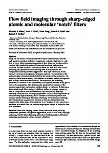
of g(yt , x ˜n ˜n ˜n t ) = gN (yt , x t ) − gF (yt , x t ) is studied. This value is returned by the filter, besides the current estimate and serves as a fault indicator (when < 0). An extension to this filter automatically adapts n by considering the decision function g variations, so n increases when a fault decision becomes more likely, and decreases otherwise. Results are presented on figure 3. The three graphs show: Middle graph The actual observations that are being tracked, the n-step predictor of state, and the Kalman filter estimate of state for a system in which a fault occurs. Top Graph The number of steps for the n-step predictor growing as the likelihood of detecting a fault grows. Bottom Graph The value at each step of the decision function. The fault is detected approximately 30 steps after it actually occurs (when the function becomes negative). When the fault detector running inside a particle detects a fault, the particle sets a timer for KT (T is the observation sampling rate) and goes to sleep. If all other particles detect a fault before this timer runs out then the particle wakes up and starts the candidate generator algorithm. If the timer expires and there are still some particles that have not indicated a fault then the particle wakes up and sets its weight to 0 and gets re-sampled. During the time that particles are asleep we continue tracking with fewer numbers of particles (total particles less the particles that are asleep).
3.3
Candidate Generator
The candidate generator is started for each particle when the fault detectors of all particles have raised a flag. Let the time when the last particle indicates a fault be tf d . Let the time of fault detection for any particle p(i) be t(i) . For each particle p(i) , we run the L3 single fault candidate generation algorithm (from assumption 3) starting at time t(i) and backtracking to time tf d − KT (from assumption 2). Note that if t(i)