Mutual Information Methods with Particle Filters for Mobile ... - CiteSeerX

Mutual Information Methods with Particle Filters for Mobile Sensor Network Control † Gabriel M. Hoffmann, Steven L. Waslander, and Claire J. Tomlin Department of Aeronautics and Astronautics Stanford University, Stanford, CA 94305 {gabeh, stevenw, tomlin}@stanford.edu Abstract— This paper develops a set of methods enabling an information-theoretic distributed control architecture based on particle filters to facilitate search by a mobile sensor network, permitting the use of nonlinear and non-Gaussian sensor models. Given a particular configuration sensors, this technique exploits the structure of the probability distributions of the target state and of the sensor measurements to compute the control inputs to the mobile sensors leading to future observations that minimize, in expectation, the future uncertainty of the target state. We compute the mutual information using a particle set representation of the posterior distribution. In order to control a large number of mobile sensors as a network, singlenode and pairwise-node approximation schemes are presented, with analytically bounded error, making the approach scalable to increasing network sizes, while still planning cooperatively. The methods are applied in simulation to bearings-only sensing, and to localizing an avalanche rescue beacon of a buried victim, using transceivers on quadrotor aircraft to measure the magnetic field. Monte Carlo simulations also demonstrate that as network size increases, the sensors more quickly localize the target, and the pairwise-node approximation results in superior performance to the single-node approximation.

I. I NTRODUCTION Mobile sensor network technology is becoming increasingly available, making it possible to exploit these platforms to efficiently and automatically search for targets with unprecedented speed, safety, and reliability. Mobile sensor network search is complicated by low prior information about the target’s state, the frequently nonlinear mapping between sensor observations and the physical world, and non-Gaussian target state representation. This paper addresses these challenges by developing a set of methods enabling an information-theoretic distributed control architecture based on particle filters. We derive methods to compute information-theoretic quantities using particle filters, and approximations that enable scalability in network size for real-time control. Given a particular configuration of sensors, this technique exploits the structure of the probability distributions of the target state and of the sensor measurements to compute control inputs leading to future observations that minimize, in expectation, the future uncertainty of the target state. The approximation schemes presented have polynomial time complexity in the network size, and analytically bounded error. The singlenode approximation leads to cooperative control due to common knowledge of the target state distribution, whereas † This research was supported by ONR under the CoMotion MURI contract N00014-02-1-0720, and by the NASA Joint University Program.

the pairwise-node approximation makes improved cooperation possible by approximating the effect of other sensing nodes’ planned observations. By using particle filters, we are able to numerically approximate the target state probability distribution, without assumptions about the family of the distribution or about the linearity of the dynamics[1]. In previous literature, one method minimizes metrics of the expected estimation covariance to compute trajectories to help estimation [2], [3]. Though computationally efficient, the approach linearizes measurement models, and relies on a Gaussian noise assumption and a guessed initial solution. This can lead to underestimation of the covariance and divergence of the filter [1], [4]. Another method, using grid cell discretization, is developed in [5], enabling use of nonlinear, non-Gaussian models. These techniques suffer poor computational time complexity with the dimension of the state, particularly for information theoretic quantities. Information theoretic costs have been used to manage sensors [6], and in [7] the expected alpha-divergence of a particle filter distribution was used for sensor management, and specialized to select modes for binary sensors, though scalability in sensor network size is not addressed. We proceed by showing equivalence of searching for a target and maximizing mutual information. Then, algorithms to compute mutual information using particle filters are then derived, and used in a distributed control algorithm to cooperatively control the vehicles. The methods are applied in simulation to localization using bearings-only sensors on airplanes, and to localization of a buried avalanche victim, using rescue beacons on quadrotor aircraft from the STARMAC project [8]. The results show successful localization under all circumstances. The pairwise-node approximation leads to faster localization than using the single-node approximation, and increasing the size of the network speeds localization. Successful localization of the rescue beacon’s magnetic field source exemplifies the utility of these techniques. II. P ROBLEM F ORMULATION A. Mobile Sensor Motion and Measurement Models Consider a set of nv vehicles carrying sensors to locate a target in the search domain, Θ. The location of the target, θ ∈ Θ ⊂ Rnθ , is unknown to the vehicles. A motion model is used for non-stationary targets [9]. A prior distribution, p0 (θ), is provided, using any information available a priori. (i) The state of the ith vehicle, at time index t, is xt ∈ Rns , with ns vehicle states. The discrete time dynamics are (i)

(i)

(i)

(i)

xt+1 = ft (xt , ut )

(1)

(i)

where ut ∈ U (i) ⊂ Rnu is the set of nu control inputs, U (i) is their domain, and the time step is ∆. A minimum (i) separation of d¯ is required between all vehicles. Let xt be th the subset of the i vehicle’s states that correspond to its position. The collision avoidance constraint is, (i) (j) ||x − x || ≥ d¯ ∀ j ∈ {1, . . . , nv : j 6= i} (2) t

t

th

(i) zt

B. Information Seeking Each vehicle, i, maintains its own minimum mean square (i) error (MMSE) estimate of the current target state, θˆt ∈ (i) nθ R , and of the posterior distribution, pt (θ ). The posterior distribution is the prior distribution conditioned on all new observations that vehicle has made or received, i.e., pt−1|t (θ(i) |z).1 These distributions, at each aircraft, based on all shared observations, can be assumed nearly identical. The main goal of a multi-vehicle search team is to minimize the total time to localize a target with a given likelihood, by making observations at some fixed rate. Therefore, the goal is to control sensor locations to minimize the expected number of future observations needed to ascertain the target’s state. A set of observations can be interpreted, in an information-theoretic sense, as a code word, with an alphabet comprised of all possible quantized outputs of the nz sensors. These encode the target state, which is represented computationally by an alphabet of a finite number of symbols, such as 64 bits in a double precision floating point data type. Therefore, to minimize the expected number of remaining observations is to maximize the expected loglikelihood of the posterior distribution with each observation of the vehicles, as derived in [10]. With constraints on control authority, the optimal observation positions may not be reachable in one time step, leading to a greedy algorithm that moves the vehicles toward the best reachable locations. In order to compute the posterior probability distribution following an observation, assuming that the target state represents the complete state of the target and the system is Markov, Bayes’ Rule can be used, 1 The

subscript of probability distribution functions indicates the time steps of the random variable arguments. For instance, pt+1|t,t+1 (a|b, c; d) is the distribution of random variable a at time t+1 conditioned on random variables b at time t and c at time t + 1, parameterized by d.

pt (θ(i) )pt+1|t (z|θ(i) ) pt (θ(i) )pt+1|t (z|θ(i) )dθ(i)

(4)

Θ

Taking the log-likelihood of each side yields (i)

(i)

(i)

H(θt |zt+1 ) = H(θt ) − I(zt+1 ; θt ) where (i) H(θt )

(i)

Sensor measurements for the i vehicle, ∈ Z ⊂ 1 . The domain of observations is R , are taken at rate ∆ Z (i) , with dimension nz . The measurement model is, (i) (i) (i) (i) zt = ht (xt , θ, ηt ) (3) provided a priori to all vehicles. The observation noise is (i) (i) ηt ∈ Rnη with assumed distribution, ηt ∼ pt (η (i) ). The noise distribution need not be Gaussian. The problem formulation admits a broad class of measurement models, as (i) ht could be a nonlinear or discontinuous mapping of the states and measurement noise onto the observation space. The vehicles are equipped with communication devices such that each vehicle can incorporate the measurements made by all other vehicles in the estimation process at each time step. One such reliable technology is demonstrated in the 802.11b network used in the STARMAC project. nz

pt+1 (θ(i) ) = R

=−

Z

pt (θ(i) ) log pt (θ(i) )dθ

(5) (6)

θ∈Θ (i)

H(θt |zRt+1 ) = − pt,t+1 (θ(i) , z) log pt|t+1 (θ(i) |z)dθdz

(7)

θ∈Θ z∈Z (i)

I(zt+1R; θt ) = pt,t+1 (θ(i) , z) log θ∈Θ z∈Z

pt,t+1 (θ (i) ,z) dθdz pt,t+1 (θ (i) )pt+1 (z)

(8)

(i)

H(θt ) is the entropy of the target state distribution, (i) I(zt+1 ; θt ) is the mutual information between the distri(i) butions of the target state and the sensors, and H(θt |zt+1 ) is the conditional entropy of the distribution — the expected entropy of the target state when conditioning with zt+1 [11]. The entropy of a probability distribution is a metric of the uncertainty of that distribution. The mutual information is a metric of the expected divergence (Kullback-Liebler) (i) between the independent and joint distributions of θt and zt+1 . It is large when two distributions have strong interdependence, and zero when they are independent. The control inputs, ut , and vehicle states, xt , influence the observations, zt+1 , through Equations (1) and (3). To minimize the expected future uncertainty of the target state distribution, with respect to ut , is to minimize Equation (5). The actual uncertainty depends on the real measurement made of zt+1 . The prior uncertainty is independent of the future control inputs, so to minimize the expected posterior uncertainty, one must maximize the observation information with respect to the control inputs. It expands as, (i)

I(zt+1 ; θt ) = H(zt+1 ) − {z } | {z } | observation information

observation uncertainty

(i)

H(zt+1 |θt ) {z } |

(9)

conditional observation uncertainty

Thus, minimizing the expected posterior uncertainty is equivalent to maximizing the difference between the uncertainty that any particular observation will be made, and the uncertainty of the measurement model. In order to seek information, the network computes its control inputs by maximizing the mutual information utility function, (i)

(i)

V (i) (xt , ut , θt ) = I(zt+1 ; θt ) as described in the next section.

(10)

III. M ETHODOLOGY A. Particle Filter Each vehicle approximates pt (θ(i) ) with an onboard particle filter, incorporating the observations shared by all ve(i) (i) hicles, with a set of N particles, (θ˜t,k , wt,k ), indexed by k, (i) (i) where θ˜t,k ∈ Θ is the state of the particle, and wt,k ∈ R+

is the likelihood weight.2 The particles approximate pt (θ(i) ) by the probability mass function, N X (i) (i) wt,k δ(θ(i) − θ˜t,k ) (11) pˆt (θ(i) ) = k=1

where δ(·) is the Dirac delta function. By maintaining a set of particles locally aboard each vehicle, only the observations need to be communicated, as opposed to the values of the entire set of particles. The particle filter iteratively incorporates new observations by predicting the state of each particle, updating the likelihood weights with the likelihood of new observations, and then resampling the particles, as described in detail in [12], [9]. A low variance sampler [4] is used for this work, with time complexity of O(N ). The MMSE estimate is Z N X (i) (i) (i) wt,k θ˜t,k (12) θˆt = θ(i) pt (θ(i) )dθ(i) ≈ k=1

Θ

B. Determining Mutual Information from Particle Sets To evaluate the mutual information utility function, Equation (10), with the particle filter representation, expand it according to Equation (9). Consider the first term, Z H(zt+1 ) = −

pt+1 (z; ut , xt ) log pt+1 (z; ut , xt )dz (13)

Z

This cannot be directly evaluated, because pt+1 (z; ut , xt ) is not available as a continuous function. Rather, the observation distribution must be determined from the particle set and sensor model. First, expand the distribution as, Z pt+1 (z; ut , xt ) = pt+1|t (z|θ(i) ; ut , xt )pt (θ(i) )dθ(i) Θ

=

Z

Θ



pt (θ(i) )

nv Y

j=1



pt+1|t (z(j) |θ(i) ; ut , xt ) dθ(i)

(14)

where the second step expands the joint distribution using the assumption that the likelihoods of sensor observations are conditionally independent given the target state distribution. This is exact when the sensors lack correlated noise. Then, Monte Carlo integration techniques can be used[13]. Substituting Equation (11) into Equation (14) yields the particle filter approximation at the ith vehicle, pt+1 (z; ut , xt ) ≈ ! nv N P (15) (i) Q (j) (i) ˜(i) pt+1|t (z |θ = θt,k ; ut , xt ) wt,k k=1

j=1

Substituting Equation (15) back into Equation (13) yields the observation entropy of the distribution represented by the particle filter approximation at the ith vehicle, H(z( t+1 ) ≈ !! nv N R P (i) Q (j) (i) ˜(i) pt+1|t (z |θ = θt,k ; ut , xt ) wt,k − j=1 k=1 Z !!) nv N P (i) Q (j) (i) ˜(i) pt+1|t (z |θ = θ ; ut , xt ) dz w · log k=1

t,k

j=1

t,k

(16)

2 The

second subscript of any variable denotes the index of the particle to which the variable belongs.

which can then be evaluated by numerical quadrature [14]. Next, similar methods are applied to compute H(zRt+1 |θt ) = − pt+1,t (z, θ(i) ; ut , xt ) log pt+1|t (z|θ(i) ; ut , xt )dzdθ(i) Z,Θ

(17) The joint distribution can be expanded using the chain rule and assuming conditional independence, nv Y (i) (i) pt+1|t (z(j) |θ(i) ; ut , xt ) pt+1,t (z, θ ; ut , xt ) = pt (θ ) j=1

(18) Substituting Equation (18) into Equation (17) and applying the approximation of Equation (11), yields the conditional observation entropy of the distribution represented by the particle filter approximation at the ith vehicle, (i)

H(zt+1 |θ (t ) ≈ nv N R P (i) (i) Q pt+1|t (z(j) |θ(i) = θ˜t,k ; ut , xt ) wt,k − j=1 Z k=1 ) nv Q (j) (i) ˜(i) pt+1|t (z |θ = θ ; ut , xt ) dz · log

(19)

t,k

j=1

Thus, the mutual information utility function, Equation (10), can be found by using Equations (16), (19), and (9). This optimization remains highly coupled between the nv vehicles. The degree of cooperation between the vehicles is analyzed to determine a scalable control strategy. C. Approximately Decoupling Mutual Information (i)

The mutual information between the random variables θt and zt+1 quantifies the expected reduction in uncertainty. However, the computational complexity of using a particle set representation to evaluate this quantity grows exponentially nz , due to integration over each dimension. We present two different approximations to mutual information that allow it to be evaluated in polynomial time with respect to the number of sensors. This makes the network scalable, yet capable of exploiting the descriptiveness of the particle filter. First, in the single-node approximation, a sensing node’s utility function uses the previous observations of all sensing nodes, but only considers its own future observations. This is a generalization of an increasingly popular technique (e.g., [2]). Second, in the pairwise-node approximation, a sensing node additionally considers the effect of plans of each other vehicle, pairwise, on the utility of its own future observation. Proposition 1: The mutual information utility function can be approximated using the single-node approximation: (i)

(i)

(i)

Vs(i) (xt , ut , θt ) = I(zt+1 ; θt ) with an error from the true value of nv   X (j) (i) (1) (j−1) (i) I(zt+1 ; zt+1 , zt+1 , . . . , zt+1 ) ǫ(i) = c + s s

(20)

(21)

j=2 j6=i

(i)

where cs encompasses the terms that are constant with respect to the ith mobile sensor’s control inputs.

Proof: Without loss of generality, consider the case of approximating the mutual information from the perspective of vehicle i = 1. The mutual information can be expanded using the chain rule [11], and then rewritten by exchanging conditioning variables (see Appendix) to yield nv P (1) (j) (1) (j−1) (1) I(θt ; zt+1 |zt+1 , . . . , zt+1 ) I(θt ; zt+1 ) = j=1 nv  P (1) (j) (1) (1) (j−1) I(θt ; zt+1 ) − I(θt ; zt+1 , . . . , zt+1 ) = j=1

Exchanging conditioning variables on the latter two terms, and canceling terms that sum to zero, (1)

(1)

(1)

I(θt ; zt+1 ) = Vs (xt , ut , θt ) + cs nv  P (j) (1) (j−1) (1) I(zt+1 ; zt+1 , . . . , zt+1 |θt ) + j=2  (j) (1) (j−1) −I(zt+1 ; zt+1 , . . . , zt+1 ) (i)

with constant cs = −

nv P

j=1 j6=i

(j)

(i)

I(zt+1 ; θt ).

Applying the assumption that observations are conditionally independent given the target state, the first term in the summation is zero. Thus, generalizing to the ith vehicle, the mutual information utility function can be evaluated using Equation (20) with error given by Equation (21). The computational complexity of the single-node approximation to the mutual information utility function is constant with respect to nv . To improve on this approximation, considering the pairwise interactions of all vehicles leads to a utility function approximation that more accurately captures the effect of group control inputs on mutual information, with computational complexity linear in nv . Proposition 2: The mutual information utility function can be approximated using the pairwise-node approximation:   (i) (i) (i) (i) Vp (xt , ut , θt ) = (2 − nv ) I(zt+1 ; θt )  nv  P (i) (j) (i) (22) I(z , z ; θt ) + j=1 j6=i

t+1

t+1

when nv ≥ 2, with an error from the true value of nv   X (j) (1) (j−1) (i) (i) I(zt+1 ; zt+1 , . . . , zt+1 |zt+1 ) ǫp =

(23)

j=2 j6=i

Proof: Without loss of generality, consider the case of approximating the mutual information from the perspective of vehicle i = 1. The mutual information can be expanded using an application of the chain rule, separating the first term in the summation, and applying the chain rule again, (1)

(1)

(1)

I(θt ; zt+1 ) = I(θt ; zt+1 )+ nv  P (j) (2) (j−1) (1) (1) I(θt ; zt+1 , zt+1 |zt+1 , . . . , zt+1 ) j=2

 (1) (1) (2) (j−1) −I(θt ; zt+1 |zt+1 , . . . , zt+1 )

(1)

(1)

(1)

I(θt ; zt+1 ) = Vp (xt , ut , θt ) nv  P (1) (2) (j−1) (1) (j) + I(θt ; zt+1 , . . . , zt+1 |zt+1 , zt+1 ) j=3

 (1) (1) (j−1) (j) +I(θt ; zt+1 , . . . , zt+1 |zt+1 )

(1)

Exchanging conditioning variables in the summation (see Appendix), canceling the resulting terms that sum to zero, and splitting the remaining summation, yields

 (j−1) (1) (1) (2) −I(θt ; zt+1 , . . . , zt+1 |zt+1 )

Exchanging conditioning variables inside the summation, canceling terms summing to zero, and assuming conditional independence of observations given the target state yields, (1) (1) (1) (1) I(θt ; zt+1 ) = Vp (xt , ut , θt ) + ǫp Thus, the mutual information utility function can be evaluated using Equation (22) with error given by Equation (23). Now we examine the effect that this added computational complexity has on the error terms, as a function of the value of the ith vehicle’s control inputs. Proposition 3: The magnitude of the error terms, that vary with the ith vehicle’s control inputs, in the single-node approximation, is greater than or equal to the magnitude of the pairwise-node approximation error terms, and equal only when the vehicle’s observations are independent of all other vehicles. That is, (i) |ǫs(i) − c(i) (24) s | ≥ |ǫp | Proof: Subtract from the single-node approximation error, Equation (21), the terms that do not vary with the (i) i(th) vehicle’s control inputs, cs , and apply the chain rule for mutual information [11], (j)

(i)

(1)

(j−1)

I(zt+1 ; zt+1 , zt+1 , . . . , zt+1 ) = (25) (j) (i) (j) (1) (j−1) (i) I(zt+1 ; zt+1 ) + I(zt+1 ; zt+1 , . . . , zt+1 |zt+1 ) Mutual information is always greater than or equal to zero, and is equal only if the distributions are independent. So, (j)

(i)

(1)

(j−1)

I(zt+1 ; zt+1 , zt+1 , . . . , zt+1 ) ≥ (j)

(2)

(j−1)

(i)

I(zt+1 ; zt+1 , . . . , zt+1 |zt+1 )

(26)

The magnitudes of the sum of the left and right sides of this equation, from j = 1 to j = nv , are equal to, respectively, the left and right sides of Equation (24). The pairwise-node approximation yields an estimate of the mutual information gain as good or better than the single-node approximation. When the vehicles’ sensors make uncorrelated measurements, the single-node approximation computes faster and yields the same result as the pairwisenode approximation. However, if the observations are correlated, as is more frequently true, then the pairwise-node approximation yields a closer estimate. Although the magnitude of the pairwise-node approximation error is less, it is not possible to guarantee that the optimization is not skewed by some systematic error between the exact solution and the single-node error. However, using the pairwisenode approximation still yields an approximate expected mutual information surpassing what seemed possible using the single-node approximation, and in experiments, the pairwisenode approximation yields better results.

D. Mobile Sensor Network Control The mobile sensor network control is structured as a set of local optimal control problems for each sensing node, coupled through interconnecting constraints. The local optimization problem is formed holding the actions of the other vehicles fixed, and an iterative algorithm is implemented based on [15] ensuring convergence to ǫ-feasible solutions that satisfy the necessary conditions for Pareto optimality. An inexact penalty function is defined for each vehicle as, (i)

(i)

(−i)

0.5

0 0

(i)

The penalty function is added to the individual vehicle cost scaled by penalty parameter β, varying the tradeoff between constraint violation and the information-theoretic cost, with an update β := αβ at each iteration, where α ∈ (0, 1) is a design parameter. The local optimization problem based on the single-node approximation, Equation (20), is

(i)

ut ∈U (i)

(i)

(i)

(i)

(−i)

(i)

(i)

(−i)

+ β1 P (xt , ut |xt (i)

(i)

(i)

(−i)

, ut

(−i)

, ut

5

10 Time

15

20

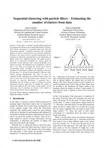
Fig. 1. Mean and quartile bars of the probability that the true target state is within 1 unit of the MMSE estimate, for sets of 1000 trials. The vehicles each make an observation at each time step. (a) Results for nv = 4. Singlenode approximation is dashed line, pairwise-node approximation is solid line. (b) Results using pairwise-node approximation for varying number of search vehicles: 2, 3, 4 and 10.

IV. A PPLICATIONS A. Bearings-Only Sensing A bearings-only sensor, such as a camera, measures the bearing to the target only. The measurement equation is, (i)

(i)

(i)

(i)

(i)

hb (x! t , θ, ηt ) = δb + ηt   (i) xt xs (i) , θ = , ηt ∼ N (0, σs2 ) (i) ys yt

(i)

)

)

(i)

subject to xt+1 = ft (xt , ut ) (i) (i) (i) (i) (i) zt+1 = ht (xt+1 , θt , ηt )

20

10 4 3 2

0 0

xt =

Single-Node Local Optimization Program: (i)

15

1

(i)

−Vs (xt , ut , θt |xt

10 Time (b)

(27)

where m indexes the set of nc interconnecting inequality constraints, g (i,m) that affect vehicle i, and −i is the set of all vehicles other than i. The penalty functions are zero wherever the constraints are satisfied, and are differentiable for all γ ≥ 2, γ ∈ R+ . The nv − 1 collision avoidance constraints from Equation (2) are rewritten as, (m) (i) g (i,m) = d¯ − ||xt+1 − xt+1 || ≤ 0 (28) ∀ m ∈ {1, . . . , nv : m 6= i}

minimize

5

0.5

(−i)

P (xt , ut |xt , ut ) = Pn(i) (i) (−i) (−i) (i,m) (i) c (xt , ut |xt , ut )γ ) m=1 max(0, g

(a) 1

(29)

The decentralized penalty method requires costs depending only on local variables, as in the single-node approximation. For the pairwise-node approximation, Equation (22), slack variables are added to decouple the local sensor costs, resulting in additional interconnecting constraints to include (i) ˜ t , as in the penalty function. Define the slack variable, u the vector of all sensors’ control inputs computed by the ith (i) ˜ t is sensor. Agreement among mobile sensing nodes on u realized through the penalty function enforced constraint, (i) (j) ˜t = u ˜t u ∀ i, j ∈ {1, . . . , nv : j 6= i} (30) The pairwise-node local optimization program is defined analogously to the single-node program, with optimization (i) ˜t ∈ U . instead over the entire control vector, u The distributed algorithm uses an iterative approach where interim solutions of control inputs are communicated amongst the vehicles in between local optimizations. This process can be hierarchical, synchronous, or asynchronous. Detailed algorithms and proof of convergence are in [15].

where δb is the angle of the ray from the ith vehicle’s (i) (i) position, (xt , yt ), to the target’s position, (xs , ys ). The additive Gaussian noise has variance σs2 . The search domain, Θ, spans a unitless 40 by 40 square. The prior distribution is uniform over the domain. The vehicles are modeled as airplanes, with fixed speeds, limited turning rates, and initially close proximity. The algorithm results in the rapid localization of the target, despite complete prior uncertainty, consistently in a large number of trials. Use of the pairwise-node approximation, Figure 1a, reduced time-to-convergence compared to the single-node approximation, on average. The pairwise-node approximation yielded more consistent performance compared to the single-node approximation, shown by narrower error bands. When applied to varying sizes of vehicle fleets, the algorithm successfully exploits the additional availability of agents, as shown in Figure 1b. The time-to-convergence is reduced, on average, as vehicles are added to the fleet. B. Rescue Beacon Sensing To rescue a victim buried in snow due to an avalanche, each vehicle uses a beacon receiver to measure the local orientation an electromagnetic (EM) field transmitted by the standard avalanche rescue beacon, carried by the victim. The position and orientation of the beacon are unknown. The magnetic field, H, of an EM source is modulated to minimize interference by snow and rocks. Measurements

(b) 40

30

30

20

20

y

y

(a) 40

10

10 20 x (c)

0 0

40

40

40

20

20

y

y

0 0

20 x (d)

40

R EFERENCES

0 0

0 20 40 0 20 40 x x Fig. 2. Four quadrotor aircraft search for a rescue beacon using the pairwise-node approximation. The particles are shown as short lines indicating position and orientation, with darkness indicating the particles’ weights. The MMSE estimate is the black X, the red dots are the vehicle waypoint history, and the red square is the true target location. Its true orientation is π . The plots (a) through (d) are at time 1, 2, 5, and 20. 4

are made of the near-field at spherical coordinates (r, ψ, φ) relative to the antenna, with components[16], i h β3 j 1 Hr = 2π cos(ψ)e−jβr + ηt,r Il (βr) 2 + (βr)3 i h j β3 1 1 sin(ψ)e−jβr + ηt,ψ Il βr − (βr) Hψ = − 4π 2 − (βr)3

where β = 2π λ is a constant of the signal modulation, I is the antenna current, l is the equivalent length, and ηt is measurement noise. Measurements of signal strength from two orthogonal antennas in the receiver give a measured direction, δ, of the field line. The measurement model is (i)

(i)

xt

(i)

(i)

(i)

(i)

hbeac (xt , θ, wt) = δ(x  t , θ, ηt ) ! xa (i) xt (i) = , θ =  ya  , ηt ∼ N (0, Σr ) (i) yt ψ a

(i) (xt ,

using particle filters. Formulae were derived to compute information-theoretic quantities using particle filters, and single-node and pairwise-node approximations were derived to enable scalability in network size. The methods were applied in simulation. The results of search using bearingsonly sensing demonstrate the utility of the techniques, and the results of search using the avalanche rescue beacon demonstrate the ability to handle problems that would pose significant hurdles to previous strategies. The techniques open the door to a variety of future applications.

(i) yt )

where is the ith vehicle’s position, and (xa , ya ) is the beacon antenna’s position, with rotation angle ψa in the horizontal plane. The covariance of the Gaussian noise is Σr . The search domain, Θ, spans a unitless 40 by 40 square, with ψa ∈ [0, 2π). The prior distribution is uniform over the domain. The search vehicle is modeled as a quadrotor aircraft [8]. They accelerate laterally proportional to their tilt, with constraints on speed, acceleration, and proximity. The proposed method quickly localizes the target, as shown in Figure 2. The quadrotors move to locations that reinforce one another’s measurements, in a behavior substantially more complicated than that required for range or bearing sensors. The posterior distribution, visualized by the particles, demonstrates the ability of this method to handle complicated posterior beliefs. It successfully exploits the structure of the distribution to reduce uncertainty. V. C ONCLUSION A set of methods were developed to enable informationtheoretic distributed control of mobile sensor network search,

[1] Gordon, N., Salmond, D., and Smith, A., “Novel approach to nonlinear/non-Gaussian Bayesian state estimation,” Radar and Signal Processing, IEE Proceedings F, Vol. 140(2), Apr 1993, pp. 107–113. [2] Grocholsky, B., Makarenko, A., and Durrant-Whyte, H., “InformationTheoretic Coordinated Control of Multiple Sensor Platforms,” Proceedings of the IEEE International Conference on Robotics and Automation, Taipei, Taiwan, Sept 2003, pp. 1521–1526. [3] Chung, T. H., Gupta, V., Burdick, J. W., and Murray, R. M., “On a Decentralized Active Sensing Strategy using Mobile Sensor Platforms in a Network,” 43rd IEEE Conference on Decision and Control, December 2004. [4] Thrun, S., Burgard, W., and Fox, D., Probabilistic Robotics, MIT Press, Cambridge, MA, 2005. [5] Bourgault, F., Furukawa, T., and Durrant-Whyte, H. F., “Decentralized Bayesian Negotiation for Cooperative Search,” Proceedings of the IEEE/RSJ International Conference on Intelligent Robotics and Systems, Sendai, Japan, September 2004, pp. 2681–2686. [6] Zhao, F., Shin, J., and Reich, J., “Information-Driven Dynamic Sensor Collaboration,” IEEE Signal Processing Magazine, March 2002, pp. 61–72. [7] Kreucher, C., Kastella, K., and III, A. O. H., “Information Based Sensor Management for Multitarget Tracking,” Proceedings of SPIE, Vol. 5204, Bellingham, WA, August 2003, pp. 480–489. [8] Waslander, S. L., Hoffmann, G. M., Jang, J. S., and Tomlin, C. J., “Multi-Agent Quadrotor Testbed Control Design: Integral Sliding Mode vs. Reinforcement Learning,” In Proceedings of the IEEE/RSJ International Conference on Intelligent Robotics and Systems 2005, Edmonton, Alberta, August 2005, pp. 468–473. [9] Gustafsson, F., Gunnarsson, F., Bergman, N., Forssell, U., Jansson, J., Karlsson, R., and Nordlund, P.-J., “Particle Filters for Positioning, Navigation and Tracking,” IEEE Transactions on Signal Processing, Vol. 50, February 2002, pp. 425–437. [10] Shannon, C. E., “A Mathematical Theory of Communication,” The Bell System Technical Journal, Vol. 27, July, October 1948, pp. 379–423, 623–656. [11] Cover, T. M. and Thomas, J. A., Elements of Information Theory, John Wiley & sons, 1991. [12] Doucet, A., de Freitas, N., and Gordon, N., editors, Sequential Monte Carlo Methods in Pracice, Statistics for Engineering and Information Science, Springer, New York, NY, 2001. [13] Bergman, N., Recursive Bayesian Estimation: navigation and tracking applications, PhD thesis 579, Link¨opings Universitet, 1999. [14] Moin, P., Fundamentals of Engineering Numerical Analysis, Cambridge University Press, 2001. [15] Inalhan, G., Stipanovic, D. M., and Tomlin, C. J., “Decentralized Optimization, with Application to Multiple Aircraft Coordination,” Proceedings of the 41st IEEE Conference on Decision and Control, Las Vegas, December 2002. [16] Narayana Rao, N., Elements of Engineering Electromagnetics, Prentice-Hall, Upper Saddle River, New Jersey, 5th ed., 2000.

A PPENDIX To exchange conditioning variables in mutual information, use random variables, a, b, and c. Then, I(a; b) − I(a; b|c) = H(a) − H(a|b) − H(a|c) + H(a|b, c) = I(a; c) − I(a; c|b) therefore, I(a; b|c) = I(a; b) − I(a; c) + I(a; c|b).