[BDL96] Clark Barrett, David Dill, and Jeremy Levitt. Validity checking for combi- nations of theories with equality. In Mandayam Srivas and Albert Camilleri,.
Invited paper for FLoC’02. Appears in the Proceedings of RTA’02, LNCS. c
Springer-Verlag
Combining Shostak Theories? Natarajan Shankar and Harald Rueß SRI International Computer Science Laboratory Menlo Park CA 94025 USA {shankar, ruess}@csl.sri.com URL: http://www.csl.sri.com/{˜shankar, ˜ruess} Phone: +1 (650) 859-5272 Fax: +1 (650) 859-2844
Abstract. Ground decision procedures for combinations of theories are used in many systems for automated deduction. There are two basic paradigms for combining decision procedures. The Nelson–Oppen method combines decision procedures for disjoint theories by exchanging equality information on the shared variables. In Shostak’s method, the combination of the theory of pure equality with canonizable and solvable theories is decided through an extension of congruence closure that yields a canonizer for the combined theory. Shostak’s original presentation, and others that followed it, contained serious errors which were corrected for the basic procedure by the present authors. Shostak also claimed that it was possible to combine canonizers and solvers for disjoint theories. This claim is easily verifiable for canonizers, but is unsubstantiated for the case of solvers. We show how our earlier procedure can be extended to combine multiple disjoint canonizable, solvable theories within the Shostak framework.
1
Introduction
Consider the sequent 2 ∗ car (x) − 3 ∗ cdr (x) = f (cdr (x)) ` f (cons(4 ∗ car (x) − 2 ∗ f (cdr (x)), y)) = f (cons(6 ∗ cdr (x), y)). ?
This work was funded by NSF Grant CCR-0082560, DARPA/AFRL Contract F33615-00-C-3043, and NASA Contract NAS1-00079. During a phone conversation with the first author on 2nd April 2001, Rob Shostak suggested that the problem of combining Shostak solvers could be solved through variable abstraction. His suggestion is the key inspiration for the combination of Shostak theories presented here. We thank Clark Barrett, Sam Owre, and Ashish Tiwari for their meticulous reading of earlier drafts. We also thank Harald Ganzinger for pointing out certain limitations of our original definition of solvability with respect to σ-models. The first author is grateful to the program committees and program chairs of the FME, LICS, and RTA conferences at FLoC 2002 for their kind invitation.
1
It involves symbols from three different theories. The symbol f is uninterpreted, the operations ∗ and − are from the theory of linear arithmetic, and the pairing and projection operations cons, car , and cdr , are from the theory of lists. There are two basic methods for building combined decision procedures for disjoint theories, i.e., theories that share no function symbols. Nelson and Oppen [NO79] gave a method for combining decision procedures through the use of variable abstraction for replacing subterms with variables, and the exchange of equality information on the shared variables. Thus, with respect to the example above, decision procedures for pure equality, linear arithmetic, and the theory of lists can be composed into a decision procedure for the combined theory. The other combination method, due to Shostak, yields a decision procedure for the combination of canonizable and solvable theories, based on the congruence closure procedure. Shostak’s original algorithm and proof were seriously flawed. His algorithm is neither terminating nor complete (even when terminating). These flaws went unnoticed for a long time even though the method was widely used, implemented, and studied [CLS96,BDL96,Bjø99]. In earlier work [RS01], we described a correct algorithm for the basic combination of a single canonizable, solvable theory with the theory of equality over uninterpreted terms. That correctness proof has been mechanically verified using PVS [FS02]. The generality of the basic combination rests on Shostak’s claim that it is possible to combine solvers and canonizers from disjoint theories into a single canonizer and solver. This claim is easily verifiable for canonizers, but fails for the case of solvers. In this paper, we extend our earlier decision procedure to the combination of uninterpreted equality with multiple canonizable, solvable theories. The decision procedure does not require the combination of solvers. We present proofs for the termination, soundness, and completeness of our procedure.
2
Preliminaries
We introduce some of the basic terminology needed to understand Shostakstyle decision procedures. Fixing a countable set of variables X and a set of function symbols F , a term is either a variable x from X or an n-ary function symbol f from F applied to n terms as in f (a1 , . . . , an ). Equations between terms are represented as a = b. Let vars(a), vars(a = b), and vars(T ) represent the sets of variables in a, a = b, and the set of equalities T , respectively. We are interested in deciding the validity of sequents of the form T ` c = d where c and d are terms, and T is a set of equalities such that vars(c = d) ⊆ vars(T ). The condition vars(c = d) ⊆ vars(T ) is there for technical reasons. It can always be satisfied by padding T with reflexivity assertions x = x for any variables x in vars(c = d) − vars(T ). We write ddaee for the set of subterms of a, which includes a. The semantics for a term a, written as M [[a]]ρ, is given relative to an interpretation M over a domain D and an assignment ρ. For an n-ary function f , the interpretation M (f ) of f in M is a map from Dn to D. For an uninterpreted 2
n-ary function symbol f , the interpretation M (f ) may be any map from Dn to D, whereas only restricted interpretations might be suitable for an interpreted function symbol like the arithmetic + operation. An assignment ρ is a map from variables in X to values in D. We define M [[a]]ρ to return a value in D by means of the following equations. M [[x]]ρ = ρ(x) M [[f (a1 , . . . , an )]]ρ = M (f )(M [[a1 ]]ρ, . . . , M [[an ]]ρ) We say that M, ρ |= a = b iff M [[a]]ρ = M [[b]]ρ, and M |= a = b iff M, ρ |= a = b for all assignments ρ. We write M, ρ |= S when ∀a, b : a = b ∈ S ⇒ M, ρ |= a = b, and M, ρ |= (T ` a = b) when (M, ρ |= T ) ⇒ (M, ρ |= a = b). A sequent T ` c = d is valid, written as |= (T ` c = d), when M, ρ |= (T ` c = d), for all M and ρ. There is a simple pattern underlying the class of decision procedures studied here. Let ψ be the state of the decision procedure as given by a set of formulas.1 τ Let τ be a family of state transformations so that we write ψ −→ ψ 0 if ψ 0 is the result of applying a transformation in τ to ψ, where vars(ψ) ⊆ vars(ψ 0 ) (variable preservation). An assignment ρ0 is said to extend ρ over vars(ψ 0 ) − vars(ψ) when it agrees with ρ on all variables except those in vars(ψ 0 ) − vars(ψ) for vars(ψ) ⊆ vars(ψ 0 ). We say that ψ 0 preserves ψ if vars(ψ) ⊆ vars(ψ 0 ) and for all interpretations M and assignments ρ, M, ρ |= ψ holds iff there exists an assignment ρ0 extending ρ such that M, ρ0 |= ψ 0 .2 When preservation is restricted to a limited class of interpretations ι, we say that ψ 0 ι-preserves ψ. Note that the preserves relation is transitive. When the operation τ is deterministic, τ (ψ) represents the result of the transformation, and we call τ a conservative operation to indicate that τ (ψ) preserves ψ for all ψ. Correspondingly, τ is said to be ιconservative when τ (ψ) ι-preserves ψ. Let τ n represent the n-fold iteration of τ , then τ n is a conservative operation. The composition τ2 ◦ τ1 of conservative operations τ1 and τ2 , is also a conservative operation. The operation τ ∗ (ψ) is defined as τ i (ψ) for the least i such that τ i+1 (ψ) = τ i (ψ). The existence of such a bound i must be demonstrated for the termination of τ ∗ . If τ is conservative, so is τ ∗ . If τ is a conservative operation, it is sound and complete in the sense that for a formula φ with vars(φ) ⊆ vars(ψ), |= (ψ ` φ) iff |= (τ (ψ) ` φ). This is clear since τ is a conservative operation and vars(φ) ⊆ vars(ψ). 1
2
In our case, the state is actually represented by a list whose elements are sets of equalities. We abuse notation by viewing such a state as the set of equalities corresponding to the union of the sets of equalities contained in it. In general, one could allow the interpretation M to be extended to M 0 in the transformation from ψ to ψ 0 to allow for the introduction of new function symbols, e.g., skolem functions. This abstract design pattern then also covers skolemization in addition to methods like prenexing, clausification, resolution, variable abstraction, and Knuth-Bendix completion.
3
If τ ∗ (ψ) returns a state ψ 0 such that |= (ψ 0 ` ⊥), where ⊥ is an unsatisfiable formula, then ψ 0 and ψ are both clearly unsatisfiable. Otherwise, if ψ 0 is canonical, as explained below, |= (ψ 0 ` φ) can be decided by computing a canonical form ψ 0 [[φ]] for φ with respect to ψ 0 .
3
Congruence Closure
In this section, we present a warm-up exercise for deciding equality over terms where all function symbols are uninterpreted, i.e., the interpretation of these operations is unconstrained. This means that a sequent T ` c = d is valid, i.e., |= (T ` c = d) iff for all interpretations M and assignments ρ, the satisfaction relation M, ρ |= (T ` c = d) holds. Whenever we write f (a1 , . . . , an ), the function symbol f is uninterpreted, and f (a1 , . . . , an ) is then said to be uninterpreted. Later on, we will extend the procedure to allow interpreted function symbols from disjoint Shostak theories such as linear arithmetic and lists. The congruence closure procedure sets up the template for the extended procedure in Section 5. The congruence closure decision procedure for pure equality has been studied by Kozen [Koz77], Shostak [Sho78], Nelson and Oppen [NO80], Downey, Sethi, and Tarjan [DST80], and, more recently, by Kapur [Kap97]. We present the congruence closure algorithm in a Shostak-style, i.e., as an online algorithm for computing and using canonical forms by successively processing the input equations from the set T . For ease of presentation, we make use of variable abstraction in the style of the abstract congruence closure technique due to Bachmair, Tiwari, and Vigneron [BTV02]. Terms of the form f (a1 , . . . , an ) are variable-abstracted into the form f (x1 , . . . , xn ) where the variables x1 , . . . , xn abstract the terms a1 , . . . , an , respectively. The procedure shown here can be seen as a specific strategy for applying the abstract congruence closure rules. In Section 5, we make essential use of variable abstraction in the Nelson–Oppen style where it is not merely a presentation device. Let T = {a1 = b1 , . . . , an = bn } for n ≥ 0 so that T is empty when n = 0. Let x and y be metavariables that range over variables. The state of the algorithm consists of a solution state S and the input equalities T . The solution state S will be maintained as the pair (SV ; SU ), where (l1 ; l2 ; . . . ; ln ) represents a list with n elements and semi-colon is an associative separator for list elements. The set SU then contains equalities of the form x = f (x1 , . . . , xn ) for an n-ary uninterpreted function f , and the set SV contains equalities of the form x = y between variables. We blur the distinction between the equality a = b and the singleton set {a = b}. Syntactic identity is written as a ≡ b as opposed to semantic equality a = b. A set of equalities R is functional if b ≡ c whenever a = b ∈ R and a = c ∈ R, for any a, b, and c. If R is functional, it can be used as a lookup table for obtaining the right-hand side entry corresponding to a left-hand side expression. Thus R(a) = b if a = b ∈ R, and otherwise, R(a) = a. The domain of R, dom(R) 4
is defined as {a | a = b ∈ R for some b}. When R is not necessarily functional, we use R({a}) to represent the set {b | a = b ∈ R ∨ b ≡ a} which is the image of {a} with respect to the reflexive closure of R. The inverse of R, written as R−1 , is the set {b = a | a = b ∈ R}. A functional set R of equalities can be applied as in R[a]. R[x] = R(x) R[f (a1 , . . . , an )] = R(f (R[a1 ], . . . , R[an ])) R[{a1 = b1 , . . . , an = bn }] = {R[a1 ] = R[b1 ], . . . , R[an ] = R[bn ]} In typical usage, R will be a solution set where the left-hand sides are all variables, so that R[a] is just the result of applying R as a substitution to a. When SV is functional, then S given by (SV ; SU ) can also be used to compute the canonical form S[[a]] of a term a with respect to S. Hilbert’s epsilon operator is used in the form of the when operator: F (x) when x : P (x) is an abbreviation for F (�x : P (x)), if ∃x : P (x). S[[x]] = SV (x) S[[f (a1 , . . . , an )]] = SV (x), when x : x = f (S[[a1 ]], . . . , S[[an ]]) ∈ SU S[[f (a1 , . . . , an )]] = f (S[[a1 ]], . . . , S[[an ]]), otherwise. The set SV of variable equalities will be maintained so that vars(SV ) ∪ vars(SU ) = dom(SV ). The set SV partitions the variables in dom(SV ) into equivalence classes. Two variables x and y are said to be in the same equivalence class with respect to SV if SV (x) ≡ SV (y). If R and R0 are solution sets and R0 is functional, then R . R0 = {a = R0 [b] | a = b ∈ R}, and R ◦ R0 = R0 ∪ (R . R0 ). The set SV is maintained in idempotent form so that SV ◦ SV = SV . Note that SU need not be functional since it can, for example, simultaneously contain the equations x = f (y), x = f (z), and x = g(y). We assume a strict total ordering x ≺ y on variables. The operation orient(x = y) returns {x = y} if x ≺ y, and returns {y = x}, otherwise. The solution state S is said to be congruence-closed if SU ({x}) ∩ SU ({y}) = ∅ whenever SV (x) 6≡ SV (y). A solution set S is canonical if S is congruence-closed, SV is functional and idempotent, and SU is normalized, i.e., SU . SV = SU . In order to determine if |= (T ` c = d), we check if S 0 [[c]] ≡ S 0 [[d]] for S 0 = process(S; T ), where S = (SV ; SU ), SV = id T , id T = {x = x | x ∈ vars(T )}, and SU = ∅. The congruence closure procedure process is defined in Figure 1. Explanation. We explain the congruence closure procedure using the validity of the sequent f (f (f (x))) = x, x = f (f (x)) ` f (x) = x as an example. Its validity will be verified by constructing a solution state S 0 equal to process(SV ; SU ; T ) for T = {f (f (f (x))) = x, x = f (f (x))}, SV = id T , SU = ∅, and checking S 0 [[f (x)]] ≡ S 0 [[x]]. Note that id T is {x = x}. In processing f (f (f (x))) = x with respect to S, the canonization step, S[[f (f (f (x))) = x]] 5
process(S; ∅) = S process(S; {a = b} ∪ T ) = process(S 0 ; T ), where, S 0 = close ∗ (merge(abstract ∗ (S; S[[a = b]]))). close(S) = merge(S; SV (x) = SV (y)), when x, y : SV (x) 6≡ SV (y), (SU ({x}) ∩ SU ({y}) 6= ∅) close(S) = S, otherwise. merge(S; x = x) = S 0 merge(S; x = y) = (SV0 ; SU ), where x 6≡ y, R = orient(x = y), 0 SV0 = SV ◦ R, SU = SU . R.
abstract(S; x = y) = (S; x = y) abstract(S; a = b) = (S 0 ; a0 = b0 ), when S 0 , a0 , b0 , x1 , . . . , xn : f (x1 , . . . , xn ) ∈ dda = bee x 6∈ vars(S; a = b) R = {x = f (x1 , . . . , xn )}, S 0 = (SV ∪ {x = x}; SU ∪ R), a0 = R−1 [a], b0 = R−1 [b]. Fig. 1. Congruence closure
yields f (f (f (x))) = x, unchanged. Next, the variable abstraction step computes abstract ∗ (f (f (f (x))) = x). First f (x) is abstracted to v1 yielding the state {x = x, v1 = v1 }; {v1 = f (x)}; {f (f (v1 )) = x}. Variable abstraction eventually terminates renaming f (v1 ) to v2 and f (v2 ) to v3 so that S is {x = x, v1 = v1 , v2 = v2 , v3 = v3 }; {v1 = f (x), v2 = f (v1 ), v3 = f (v2 )}. The variable abstracted input equality is then v3 = x. Let orient(v3 = x) return v3 = x. Next, merge(S; v3 = x) yields the solution state {x = x, v1 = v1 , v2 = v2 , v3 = x}; {v1 = f (x), v2 = f (v1 ), v3 = f (v2 )}. The congruence closure step close ∗ (S) leaves S unchanged since there are no variables that are merged in SU and not in SV . The next input equality x = f (f (x)) is canonized as x = v2 which can be oriented as v2 = x and merged with S to yield the new value {x = x, v1 = v1 , v2 = x, v3 = x}; {v1 = f (x), v2 = f (v1 ), v3 = f (x)} for S. The congruence closure step close ∗ (S) now detects that v1 and v3 are merged in SU but not in SV and generates the equality v1 = v3 . This equality is merged to yield the new value of S as {x = x, v1 = x, v2 = x, v3 = x}; {v1 = f (x), v2 = f (x), v3 = f (x)}, which is congruence-closed. With respect to this final value of the solution state S, it can be checked that S[[f (x)]] ≡ x ≡ S[[x]].
6
Invariants. The Shostak-style congruence closure algorithm makes heavy use of canonical forms and this requires some key invariants to be preserved on the solution state S. If vars(SV )∪vars(SU ) ⊆ dom(SV ), then vars(SV0 )∪vars(SU0 ) ⊆ dom(SV0 ), when S 0 is either abstract(S; a = b) or close(S). If S is canonical and a0 = S[[a]], then SV [a0 ] = a0 . If SU . SV = SU , SV [a] = a, and SV [b] = b, then SU0 . SV0 = SU0 where S 0 ; a0 = b0 is abstract(S; a = b). Similarly, if SU . SV = SU , SV (x) ≡ x, SV (y) ≡ y, then SU0 ◦ SV0 = SU0 for S 0 = merge(S; x = y). If SV is functional and idempotent, then so is SV0 , where S 0 is either of abstract(S; a = b) or close(S). If S 0 = close ∗ (S), then S 0 is congruence-closed, and if SV is functional and idempotent, SU is normalized, then S 0 is canonical. Variations. In the merge operation, if SU0 is computed as R[SU ] instead of SU . R, this would preserve the invariant that SU−1 is always functional and SV [SU ] = SU . If this is the case, the canonizer can be simplified to just return SU−1 (f (S[[a1 ]], . . . , S[[an ]])). Termination. The procedure process(S; T ) terminates after each equality in T has been asserted into S. The operation abstract ∗ terminates because each recursive call decreases the number of occurrences of function applications in the given equality a = b by at least one. The operation close ∗ terminates because each invocation of the merge operation merges two distinct equivalence classes of variables in SV . The process operation terminates because the number of input equations in T decreases with each recursive call. Therefore the computation of process(S; T ) terminates returning a canonical solution set S 0 . Soundness and Completeness. We need to show that |= (T ` c = d) ⇐⇒ S 0 [[c]] ≡ S 0 [[d]] for S 0 = process(id T ; ∅; T ) and vars(c = d) ⊆ vars(T ). We do this by showing that S 0 preserves (id T ; ∅; T ), and hence |= (T ` c = d) ⇐⇒ |= (S 0 ` c = d), and |= (S 0 ` c = d) ⇐⇒ S 0 [[c]] ≡ S 0 [[d]]. We can easily establish that if process(S; T ) = S 0 , then S 0 preserves (S; T ). If a0 = b0 is obtained from a = b by applying equality replacements from S, then (S; a0 = b0 ) preserves (S; a = b). In particular, |= (S ` S[[c]] = c) holds. The following claims can then be easily verified. 1. 2. 3. 4.
(S; S[[a = b]]) preserves (S; a = b). abstract(S; a = b) preserves (S; a = b). merge(S; a = b) preserves (S; a = b). close(S) preserves S.
The only remaining step is to show that if S 0 is canonical, then |= (S 0 ` c = d) ⇐⇒ S 0 [[c]] ≡ S 0 [[d]] for vars(c = d) ⊆ vars(S). Since we know that |= S 0 ` S 0 [[c]] = c and |= S 0 ` S 0 [[d]] = d, hence |= (S 0 ` c = d) follows from S 0 [[c]] ≡ S 0 [[d]]. For the only if direction, we show that if S 0 [[c]] 6≡ S 0 [[d]], then there is an interpretation MS 0 and assignment ρS 0 such that MS 0 , ρS 0 |= S but MS 0 , ρS 0 6|= c = d. A canonical term (in S’) is a term a such that S 0 [[a]] ≡ a. The domain DS 0 is taken to be the set of canonical terms built from the function symbols F and variables from vars(S 0 ). We constrain MS 0 so that MS 0 (f )(a1 , . . . , an ) = SV0 (x) 7
when there is an x such that x = f (a1 , . . . , an ) ∈ SU0 , and f (a1 , . . . , an ), otherwise. Let ρS 0 map x in vars(S 0 ) to SV0 (x); the mappings for the variables outside vars(S 0 ) are irrelevant. It is easy to see that MS 0 [[c]]ρS 0 = S 0 [[c]] by induction on the structure of c. In particular, when S 0 is canonical, MS 0 (f )(x1 . . . , xn ) = x for x = f (x1 , . . . , xn ) ∈ SU0 , so that one can easily verify that MS 0 , ρS 0 |= S 0 . Hence, if S 0 [[c]] 6≡ S 0 [[d]], then 6|= (S 0 ` c = d).
4
Shostak Theories
A Shostak theory [Sho84] is a theory that is canonizable and solvable. We assume a collection of Shostak theories θ1 , . . . , θN . In this section, we give a decision procedure for a single Shostak theory θi , but with i as a parameter. This background material is adapted from Shankar [Sha01]. Satisfiability M, ρ |= a = b is with respect to i-models M . The equality a = b is i-valid, i.e., |=i a = b, if for all imodels M and assignments ρ, M [[a]]ρ = M [[b]]ρ. Similarly, a = b is i-unsatisfiable, i.e., |=i a 6= b, when for all i-models M and assignments ρ, M [[a]]ρ 6= M [[b]]ρ. An i-term a is a term whose function symbols all belong to θi and vars(a) ⊆ X ∪ Xi . A canonizable theory θi admits a computable operation σi on terms such that |=i a = b iff σi (a) ≡ σi (b), for i-terms a and b. An i-term a is canonical if σi (a) ≡ a. Additionally, vars(σi (a)) ⊆ vars(a) and every subterm of σi (a) must be canonical. For example, a canonizer for the theory θA of linear arithmetic can be defined to convert expressions into an ordered sum-of-monomials form. Then, σA (y + x + x) ≡ 2 ∗ x + y ≡ σA (x + y + x). A solvable theory admits a procedure solve i on equalities such that solve i (Y )(a = b) for a set of variables Y with vars(a = b) ⊆ Y , returns a solved form for a = b as explained below. solve i (Y )(a = b) might contain fresh variables that do not appear in Y . A functional solution set R is in i-solved form if it is of the form {x1 = t1 , . . . , xn = tn }, where for j, 1 ≤ j ≤ n, tj is a canonical i-term, σi (tj ) ≡ tj , and vars(tj ) ∩ dom(R) = ∅ unless tj ≡ xj . The i-solved form solve i (Y )(a = b) is either ⊥i , when |=i a 6= b, or is a solution set of equalities which is the union of sets R1 and R2 . The set R1 is the solved form {x1 = t1 , . . . , xn = tn } with xj ∈ vars(a = b) for 1 ≤ j ≤ n, and for any i-model M and assignment ρ, we have that M, ρ |= a = b iff there is a ρ0 extending ρ over vars(solve i (Y )(a = b)) − Y such that M, ρ0 |= xj = tj , for 1 ≤ j ≤ n. The set R2 is just {x = x | x ∈ vars(R1 ) − Y } and is included in order to preserve variables. In other words, solve i (Y )(a = b) i-preserves a = b. For example, a solver for linear arithmetic can be constructed to isolate a variable on one side of the equality through scaling and cancellation. We assume that the fresh variables generated by solve i are from the set Xi . We take vars(⊥i ) to be X ∪ Xi so as to maintain variable preservation, and indeed ⊥i could be represented as just ⊥ were it not for this condition. We now describe a decision procedure for sequents of the form T ` c = d in a single Shostak theory with canonizer σi and solver solve i . Here the solution state 8
S is just a functional solution set of equalities in i-solved form. Given a solution set S, we define Shhaiii as σi (S[a]). The composition of solutions sets is defined so that S ◦i ⊥i = ⊥i ◦i S = ⊥i and S ◦i R = R ∪ {a = Rhhbiii | a = b ∈ S}. Note that solved forms are idempotent with respect to composition so that S ◦i S = S. The solved form solveclose i (id T ; T ) is obtained by processing the equations in T to build up a solution set S. An equation a = b is first canonized with respect to S as Shhaiii = Shhbiii and then solved to yield the solution R. If R is ⊥i , then T is i-unsatisfiable and we return the solution state with Si = ⊥i as the result. Otherwise, the composition S ◦i R is computed and used to similarly process the remaining formulas in T . solveclose i (S; ∅) = S solveclose i (⊥i ; T ) = ⊥i solveclose i (S; {a = b} ∪ T ) = solveclose i (S 0 , T ), where S 0 = S ◦i solve i (vars(S))(Shhaiii = Shhbiii ) To check i-validity, |=i (T ` c = d), it is sufficient to check that either solveclose i (id T ; T ) = ⊥ or S 0 hhciii ≡ S 0 hhdiii , where S 0 = solveclose i (id T ; T ). Soundness and Completeness. As with the congruence closure procedure, each step in solveclose i is i-conservative. Hence solveclose i is sound and complete: if S 0 = solveclose i (S; T ), then for every i-model M and assignment ρ, M, ρ |= S∪T iff there is a ρ0 extending ρ over the variables in vars(S 0 ) − vars(S) such that M, ρ0 |= S 0 . If σi (S 0 [a]) ≡ σi (S 0 [b]), then M, ρ0 |= a = S 0 [a] = σi (S 0 [a]) = σi (S 0 [b]) = S 0 [b] = b, and hence M, ρ |= a = b. Otherwise, when σi (S 0 [a]) 6≡ σi (S 0 [b]), we know by the condition on σi that there is an i-model M and an assignment ρ0 such that M [[S 0 [a]]]ρ0 6= M [[S 0 [b]]]ρ0 . The solved form S 0 divides the variables into independent variables x such that S 0 (x) = x, and dependent variables y where y 6= S 0 (y) and the variables in vars(S 0 (y)) are all independent. We can therefore extend ρ0 to an assignment ρ where the dependent variables y are mapped to M [[S 0 (y)]]ρ0 . Clearly, M, ρ |= S 0 , M, ρ |= a = S 0 [a], and M, ρ |= b = S 0 [b]. Since S 0 i-preserves (id T ; T ), M, ρ |= T but M, ρ 6|= a = b and hence T ` a = b is not i-valid, so the procedure is complete. The correctness argument is thus similar to that of Section 3 but for the case of a single Shostak theory considered here, there is no need to construct a canonical term model since |=i a = σi (a), and σi (a) ≡ σi (b) iff |=i a = b. Canonical term model. The situation is different when we wish to combine Shostak theories. It is important to resolve potential semantic incompatibilities between two Shostak theories. With respect to some fixed notion of i-validity for θi and j-validity for θj with i 6= j, a formula A in the union of θi and θj may be satisfiable in an i-interpretation of only a specific finite cardinality for which there might be no corresponding satisfying j-interpretation for the formula. Such an incompatibility can arise even when a theory θi is extended with uninterpreted function symbols. For example, if φ is a formula with variables x and y that is satisfiable only in a two-element model M where ρ(x) 6= ρ(y), then 9
the set of formulas Γ where Γ = {φ, f (x) = x, f (u) = y, f (y) = x} additionally requires ρ(x) 6= ρ(u) and ρ(y) 6= ρ(u). Hence, a model for Γ must have at least three elements, so that Γ is unsatisfiable. However, there is no way to detect this kind of unsatisfiability purely through the use of solving and canonization. We introduce a canonical term model as a way around such semantic incompatibilities. The set of canonical i-terms a such that σi (a) ≡ a yields a domain for a term model Mi where Mi (f )(a1 , . . . , an ) = σi (f (a1 , . . . , an )). If Mi is (isomorphic to) an i-model, then we say that the theory θi is composable. Note that the solve operation is conservative with respect to the model Mi as well, since Mi is taken as an i-model. Given the usual interpretation of disjunction, a notion of validity is said to be convex when |= (T ` c1 = d1 ∨ . . . ∨ cn = dn ) implies |= (T ` ck = dk ) for some k, 1 ≤ k ≤ n. If a theory θi is composable, then i-validity is convex. Recall that |=i (T ` c1 = d1 ∨ . . . ∨ cn = dn ) iff |=i (S ` c1 = d1 ∨ . . . ∨ cn = dn ) for S = solveclose i (id T ; T ). If S = ⊥i , then |=i (T ` ck = dk ), for 1 ≤ k ≤ n. If S 6= ⊥i , then since S i-preserves T , |=i (S ` c1 = d1 ∨ . . . ∨ cn = dn ), but (by assumption) 6|=i (S ` ck = dk ). An assignment ρS can be constructed so that for independent ( i.e., where S(x) = x) variables x ∈ vars(S), ρS (x) = x, and for dependent variables y ∈ vars(S), ρS (y) = Mi [[S(y)]]ρS . If for S 6= ⊥i , 6|=σi (S ` ck = dk ), then Mi , ρS |= S and Mi , ρS 6|= ck = dk . Hence Mi , ρS 6|= (S ` ck = dk ), for 1 ≤ k ≤ n. This yields Mi , ρS 6|= (T ` c1 = d1 ∨ . . . ∨ cn = dn ), contradicting the assumption.
5
Combining Shostak Theories
We now examine the combination of the theory of equality over uninterpreted function symbols with several disjoint Shostak theories. Examples of interpreted operations from Shostak theories include + and − from the theory of linear arithmetic, select and update from the theory of arrays, and cons, car , and cdr from the theory of lists. The basic Shostak combination algorithm covers the union of equality over uninterpreted function symbols and a single canonizable and solvable equational theory [Sho84,CLS96,RS01]. Shostak [Sho84] had claimed that the basic combination algorithm was sufficient because canonizers and solvers for disjoint theories could be combined into a single canonizer and solver for their union. This claim is incorrect.3 We present a combined decision procedure for multiple Shostak theories that overcomes the difficulty of combining solvers. Two theories θ1 and θ2 are said to be disjoint if they have no function symbols in common. A typical subgoal in a proof can involve interpreted symbols from several theories. Let σi be the canonizer for θi . A term f (a1 , . . . , an ) is said to be in θi if f is in θi even though some ai might contain function symbols outside θi . In processing terms from the union of pairwise disjoint theories θ1 , . . . , θN , 3
The difficulty with combining Shostak solvers was observed by Jeremy Levitt [Lev99].
10
it is quite easy to combine the canonizers so that each theory treats terms in the other theory as variables. Since σi is only applicable to i-terms, we first have to extend the canonizer σi to treat terms in θj for j 6= i, as variables. Let πi be a chosen bijective set of equalities between the variables X and the set {a|(∃j : j 6= i ∧ a ∈ θj )}. We treat uninterpreted function symbols as belonging to a special theory θ0 where σ0 (a) = a for a ∈ θ0 . The extended operation σi0 is defined below. σi0 (a) = πi [σi (a0 )], when a0 : a0 is an i-term, πi [a0 ] ≡ a. Note that the when condition in the above definition can always be satisfied. The combined canonizer σ can then be defined as σ(x) = x σ(f (a1 , . . . , an )) = σi0 (f (σ(a1 ), . . . , σ(an ))), when i : f is in θi . This canonizer is, however, not used in the remainder of the paper. We now discuss the difficulty of combining the solvers solve 1 and solve 2 for θ1 and θ2 , respectively, into a single solver. The example uses the theory θA of linear arithmetic and the theory θL of the pairing and projection operations cons, car , cdr , where, somewhat nonsensically, the projection operations also apply to numerical expressions. Shostak illustrated the combination using the example 5 + car (x + 2) = cdr (x + 1) + 3. Since the top-level operation on the left-hand side is +, we can treat car (x + 2) and cdr (x + 1) as variables and use solve A . This might yield a partially solved equation of the form car (x + 2) = cdr (x + 1) − 2. Now since the top-level operation on the left-hand side is from the theory of lists, we use solve L to obtain x + 2 = cons(cdr (x + 1) − 2, u) with a fresh variable u. We once again apply solve A to obtain x = cons(cdr (x + 1) − 2, u) − 2. This is, however, not in solved form: the left-hand side variable occurs in an interpreted context in its solution. There is no way to prevent this from happening as long as each solver treats terms from another theory as variables. Therefore the union of Shostak theories is not necessarily a Shostak theory. The problem of combining disjoint Shostak theories actually has a very simple solution. There is no need to combine solvers. Since the theories are disjoint, the canonizer can tolerate multiple solutions for the same variable as long as there is at most one solution from any individual theory. This can be illustrated on the same example: 5 + car (x + 2) = cdr (x + 1) + 3. By variable abstraction, we obtain the equation v3 = v6 , where v1 = x + 2, v2 = car (v1 ), v3 = v2 + 5, v4 = x + 1, v5 = cdr (v4 ), v6 = v5 + 3. We can separate these equations out into the respective theories so that S is (SV ; SU ; SA ; SL ), where SV contains the variable equalities in canonical form, SU is as in congruence closure but is always ∅ since there are no uninterpreted operations in this example, and SA and SL are the 11
solution sets for θA and θL , respectively. We then get SV = {x = x, v1 = v1 , v2 = v2 , v3 = v6 , v4 = v4 , v5 = v5 , v6 = v6 }, SA = {v1 = x + 2, v3 = v2 + 5, v4 = x + 1, v6 = v5 + 3}, and SL = {v2 = car (v1 ), v5 = cdr (v4 )}. Since v3 and v6 are merged in SV , but not in SA , we solve the equality between SA (v3 ) and SA (v6 ), i.e., solve A (v2 + 5 = v5 + 3) to get v2 = v5 − 2. This result is composed with SA to get {v1 = x + 2, v3 = v5 + 3, v4 = x + 1, v6 = v5 + 3, v2 = v5 − 2} for SA . There are no new variable equalities to be propagated out of either SA , SL , or SV . Notice that v2 and v5 both have different solved forms in SA and SL . This is tolerated since the solutions are from disjoint theories and the canonizer can pick a solution that is appropriate to the context. For example, when canonizing a term of the form f (x) for f ∈ θi , it is clear that the only relevant solution for x is the one from Si . We can now check whether the resulting solution state verifies the original equation 5 + car (x + 2) = cdr (x + 1) + 3. In canonizing f (a1 , . . . , an ) we return SV (y) whenever the term f (Si (S[[a1 ]]), . . . , Si (S[[an ]])) being canonized is such that y = f (Si (S[[a1 ]]), . . . , Si (S[[an ]])) ∈ Si for f ∈ θi . Thus x + 2 canonizes to v1 using SA , and car (v1 ) canonizes to v2 using SL . The resulting term 5 + v2 , using the solution for v2 from SA , simplifies to v5 + 3, which returns the canonical form v6 by using SA . On the right-hand side, x + 1 is equivalent to v4 in SA , and car (v4 ) simplifies to v5 using SL The right-hand side therefore simplifies to v5 +3 which is canonized to v6 using SA . The canonized left-hand and right-hand sides are identical. We present a formal description of the procedure used informally in the above example. We show how process from Section 3 can be extended to combine the union of disjoint solvable, canonizable, composable theories. We assume that there are N disjoint theories θ1 ,. . . , θN . Each theory θi is equipped with a canonizer σi and solver solve i for i-terms. If we let I represent the interval [1, N ], then an I-model is a model M that is an i-model for each i ∈ I. We will ensure that each inference step is conservative with respect to I-models, i.e., I-conservative. We represent the uninterpreted part of S as S0 instead of SU . The solution state S of the algorithm now consists of a list of sets of equations (SV ; S0 ; S1 ; . . . ; SN ). Here SV is a set of variable equations of the form x = y, and S0 is the set of equations of the form x = f (x1 , . . . , xn ) where f is uninterpreted. Each Si is in i-solved form and is the solution set for θi . Terms now contain a mixture of function symbols that are uninterpreted or are interpreted in one of the theories θi . A solution state S is confluent if for all x, y ∈ dom(SV ) and i, 0 ≤ i ≤ N : SV (x) ≡ SV (y) ⇐⇒ Si ({x}) ∩ Si ({y}) 6= ∅. A solution state S is canonical if it is confluent; SV is functional and idempotent, i.e., SV ◦SV = SV ; the uninterpreted solution set S0 is normalized, i.e., S0 .SV = S0 ; each Si , for i > 0, is functional, idempotent, i.e., Si ◦i Si = Si , normalized i.e., Si . SV = Si , and in i-solved form. The canonization of expressions with respect to a canonical solution set S is defined as follows. 4
S[[x]] = SV (x)
12
abstract(S; x = y) = (S; x = y), abstract(S; a = b) = (S 0 ; a0 = b0 ), when S 0 , c, i : c ∈ max (dda = beei ), x 6∈ vars(S ∪ a = b), SV0 = SV ∪ {x = x}, Si0 = Si ∪ {x = c}, Sj0 = Sj , for , i 6= j a0 = S 0 [[a]], b0 = S 0 [[b]]. Fig. 2. Variable abstraction step for multiple Shostak theories
4
S[[f (a1 , . . . , an )]] = SV (x), when i, x : i > 0, f ∈ θi , x = S{{f (a1 , . . . , an )}} ∈ Si 4
S[[f (a1 , . . . , an )]] = S{{f (a1 , . . . , an )}}, otherwise. 4
S{{f (a1 , . . . , an )}} = σi0 (f (Si (S[[a1 ]]), . . . , Si (S[[an ]]))), if f ∈ θi , i > 0 4
S{{f (a1 , . . . , an )}} = f (S[[a1 ]], . . . , S[[an ]]), if f ∈ θ0 . Since variables are used to communicate between the different theories, the canonical variable x in SV is returned when the term being canonized is known to be equivalent to an expression a such that y = a in Si , where x ≡ SV (y). The definition of the above global canonizer is one of the key contributions of this paper. This definition can be applied to the example above of computing S[[5 + car (x + 2)]]. Variable Abstraction. The variable abstraction procedure abstract(S; a = b) is shown in Figure 2. If a is an i-term such that a 6∈ X, then a is said to be a pure i-term. Let dda = beei represent the set of subterms of a = b that are pure i-terms. A maximal 0-term is one of the form f (x1 , . . . , xn ) for f ∈ θ0 . For i > 0, the set max (M ) of maximal terms in M is defined to be {a ∈ M |a ≡ b ∨ a 6∈ ddbee, for any b ∈ M }. In a single variable abstraction step, abstract(S; a = b) picks a maximal pure i-subterm c from the canonized input equality a = b, and replaces it with a fresh variable x from X while adding x = c to Si . By abstracting a maximal pure i-term, we ensure that Si remains in i-solved form. Explanation. The procedure in Figure 3 is similar to that of Figure 1. Equations from the input set T are processed into the solution state S of the form SV ; S0 ; . . . , SN . Initially, S must be canonical. In processing the input equation a = b into S, we take steps to systematically restore the canonicity of S. The first step is to compute the canonical form S[[a = b]] of a = b with respect to S. It is easy to see that (S; S[[a = b]]) I-preserves (S; a = b). 13
process(S; ∅) = S process(S; T ) = S, when i : Si = ⊥i process(S; {a = b} ∪ T ) = process(S 0 ; T ), where S 0 = close ∗ (merge V (abstract ∗ (S; S[[a = b]]))). close(S) = S, when i : Si = ⊥i close(S) = S 0 , when S 0 , i, x, y : x, y ∈ dom(SV ), (i > 0, SV (x) ≡ SV (y), Si (x) 6≡ Si (y), and S 0 = merge i (S; x = y)) or (i ≥ 0, SV (x) 6≡ SV (y), Si ({x}) ∩ Si ({y}) 6= ∅, and S 0 = merge V (S; SV (x) = SV (y))) close(S) = normalize(S), otherwise. normalize(S) = (SV ; S0 ; S1 . SV ; . . . ; SN . SV ). merge i (S; x = y) = S 0 , where i > 0, Si0 = Si ◦i solve i (vars(Si ))(Si (x) = Si (y)), Sj0 = Sj , for i 6= j, SV0 = SV . merge V (S; x = x) = S merge V (S; x = y) = (SV ◦ R; S0 . R; S1 ; . . . ; SN ), where R = orient(x = y). Fig. 3. Combining Multiple Shostak Theories
The result of the canonization step a0 = b0 is then variable abstracted as abstract ∗ (a0 = b0 ) (shown in Figure 2) so that in each step, a maximal, pure i-subterm c of a0 = b0 is replaced by a fresh variable x, and the equality x = c is added to Si . This is also easily seen to be an I-conservative step. The equality x = y resulting from the variable abstraction of a0 = b0 is then merged into SV and S0 . This can destroy confluence since there may be variables w and z such that w and z are merged in SV (i.e., SV (w) ≡ SV (z)) that are unmerged in some Si (i.e., Si ({w}) ∩ Si ({z}) = ∅), or vice-versa.4 The number of variables in dom(SV ) remains fixed during the computation of close ∗ (S). Confluence is restored by close ∗ (S) which finds a pair of variables that are merged in some Si but not in SV , and merging them in SV , or that are merged in SV and not in some Si and merging them in Si . Each such merge step is also I-conservative. When this process terminates, S is once again canonical. The solution sets Si are normalized with respect to SV in order to ensure that the entries are in the normalized form for lookup during canonization. 4
For i > 0, Si is maintained in i-solved form and hence, Si ({x}) = {x, Si (x)}.
14
Invariants. As with congruence closure, several key invariants are needed to ensure that the solution state S is maintained in canonical form whenever it is given as the argument to process. If S is canonical and a and b are canonical with respect to S, then for (S 0 ; a0 = b0 ) = abstract(S; a = b), S 0 is canonical, and a0 and b0 are canonical with respect to S 0 . The state abstract(S; a = b) Ipreserves (S; a = b). A solution state is said to be well-formed if SV is functional and idempotent, S0 is normalized, and each Si is functional, idempotent, and in solved form. Note that if S is well-formed, confluent, and each Si is normalized, then it is canonical. When S is well-formed, and S 0 = merge V (S; x = y) or S 0 = merge i (S; x = y), then S 0 is well-formed and I-preserves (S; x = y). If S is well-formed and congruence-closed, and S 0 = normalize(S), then S 0 is wellformed and each Si0 is normalized. If S 0 = normalize(S), then each Si0 is in solved form because if x replaces y on the right-hand side of a solution set Si , then Si (y) ≡ y since Si is in i-solved form. By congruence closure, we already have that Si (x) ≡ Si (y) ≡ y. Therefore, the uniform replacement of y by x ensures that Si0 (x) ≡ x, thus leaving S in solved form. If S 0 = close ∗ (S), where S is well-formed, then S 0 is canonical. Variations. As with congruence closure, once S is confluent, it is safe to strengthen the normalization step to replace each Si by SV [Si ]. This renders S0−1 functional, but Si−1 may still be non-functional for i > 0, since it might contain left-hand side variables that are local. However, if Sˆi is taken to be Si restricted to dom(SV ), then Sˆi−1 with the strengthened normalization is functional and can be used in canonization. The solutions for local variables can be safely discarded in an actual implementation. The canonization and variable abstraction steps can be combined within a single recursion. Termination. The operations S[[a = b]] and abstract ∗ (S; a = b) are easily seen to be terminating. The operation close ∗ (S) also terminates because the sum of the number of equivalence classes of variables in dom(SV ) with respect to each of the solution sets SV , S0 , S1 , . . . , SN , decreases with each merge operation. Soundness and Completeness. We have already seen that each of the steps: canonization, variable abstraction, composition, merging, and normalization, is I-conservative. It therefore follows that if S 0 = process(S; T ), then S 0 Ipreserves S. Hence, if S 0 [[c]] ≡ S 0 [[d]], then clearly |=I (S 0 ` c = d), and hence |=I (S; T ` c = d). The completeness argument requires the demonstration that if S 0 [[c]] 6≡ S 0 [[d]], then 6|=I (S 0 ` c = d) when S 0 is canonical. This is done by means of a construction of MS 0 and ρS 0 such that MS 0 , ρS 0 |= S 0 but MS 0 , ρS 0 6|= c = d. The domain D consists of canonical terms e such that S 0 [[e]] = e. As with congruence closure, MS 0 is defined so that MS 0 (f )(e1 , . . . , en ) = S 0 [[f (e1 , . . . , en )]]. The assignment ρS 0 is defined so that ρS 0 (x) = SV (x). By induction on c, we have that MS 0 [[c]]ρS 0 = S 0 [[c]]. We can also easily check that MS 0 , ρS 0 |= S 0 . It is also the case that MS 0 is an I-model since MS 0 is isomorphic to Mi for each i, 1 ≤ i ≤ N . This can be demonstrated by constructing a bijective 15
map µi between D and the domain Di corresponding to Mi so that µi (x) = a0 , where πi [a0 ] = SI (x), µi (f (a1 , . . . , an )) = f (µi (a1 ), . . . , µi (an )) if f ∈ θi , and πi−1 (f (a1 , . . . , an ), otherwise. It can then be verified that for any f ∈ θi and terms a1 , . . . , an in D, µi (MS 0 (f )(a1 , . . . , an )) = Mi (f )(µi (a1 ), . . . , µi (an )). This concludes the proof of completeness. Convexity revisited. As in Section 4, the term model construction of MS 0 once again establishes that I-validity is convex. In other words, a sequent |=I (T ` c1 = d1 ∨ . . . ∨ cn = dn ) iff |=I (T ` ck = dk ) for some k, 1 ≤ k ≤ n.
6
Conclusions
Ground decision procedures for equality are crucial for discharging the myriad proof obligations that arise in numerous applications of automated reasoning. These goals typically contain operations from a combination of theories, including uninterpreted symbols. Shostak’s basic method deals only with the combination of a single canonizable, solvable theory with equality over uninterpreted function symbols. Indeed, in all previous work based on Shostak’s method, only the basic combination is considered. Though Shostak asserted that the basic combination was adequate to cover the more general case of multiple Shostak theories, this claim has turned out to be unsubstantiated. We have given here the first Shostak-style combination method for the general case of multiple Shostak theories. The algorithm is quite simple and is supported by straightforward arguments for termination, soundness, and completeness. Shostak’s combination method, as we have described it, is clearly an instance of a Nelson–Oppen combination [NO79] since it involves the exchange of equalities between variables through the solution set SV . The added advantage of a Shostak combination is that it combines the canonizers of the individual theories into a global canonizer. The definition of such a canonizer for multiple Shostak theories is the key contribution of this paper. The technique of achieving confluence across the different solution sets is unique to our method. Confluence is needed for obtaining useful canonical forms, and is therefore not essential in a general Nelson–Oppen combination. The global canonizer S[[a]] can be applied to input formulas to discharge queries and simplify input formulas. The reduction to canonical form with respect to the given equalities helps keep the size of the term universe small, and makes the algorithm more efficient than a black box Nelson–Oppen combination. The decision algorithm for a Shostak theory given in Section 4 fits the requirements for a black box procedure that can be used within a Nelson–Oppen combination. The Nelson–Oppen combination of Shostak theories with other decision procedures has been studied by Tiwari [Tiw00], Barrett, Dill, and Stump [BDS02], and Ganzinger [Gan02], but none of these methods includes a general canonization procedure as is required for a Shostak combination.
16
Variable abstraction is also used in the combination unification procedure of Baader and Schulz [BS96], which addresses a similar problem to that of combining Shostak solvers. In our case, there is no need to ensure that solutions are compatible across distinct theories. Furthermore, variable dependencies can be cyclic across theories so that it is possible to have y ∈ vars(Si (x)) and x ∈ vars(Sj (y)) for i 6= j. Our algorithm can be easily and usefully adapted for combining unification and matching algorithms with constraint solving in Shostak theories. Insights derived from the Nelson–Oppen combination method have been crucial in the design of our algorithm and its proof. Our presentation here is different from that of our previous algorithm for the basic Shostak combination [RS01] in the use of variable abstraction and the theory-wise separation of solution sets. Our proof of the basic algorithm additionally demonstrated the existence of proof objects in a sound and complete proof system. This can easily be replicated for the general algorithm studied here. The soundness and completeness proofs given here are for composable theories and avoid the use of σ-models. Our Shostak-style algorithm fits modularly within the Nelson–Oppen framework. It can be employed within a Nelson–Oppen combination (as suggested by Rushby [CLS96]) in which there are other decision procedures that generate equalities between variables. It is also possible to combine it with decision procedures that are not disjoint, as for example with linear arithmetic inequalities. Here, the existence of a canonizer with respect to equality is useful for representing inequality information in a canonical form. A variant of the procedure described here is implemented in ICS [FORS01] in exactly such a combination.
References [BDL96] Clark Barrett, David Dill, and Jeremy Levitt. Validity checking for combinations of theories with equality. In Mandayam Srivas and Albert Camilleri, editors, Formal Methods in Computer-Aided Design (FMCAD ’96), volume 1166 of Lecture Notes in Computer Science, pages 187–201, Palo Alto, CA, November 1996. Springer-Verlag. [BDS02] Clark W. Barrett, David L. Dill, and Aaron Stump. A generalization of Shostak’s method for combining decision procedures. In A. Armando, editor, Frontiers of Combining Systems, 4th International Workshop, FroCos 2002, number 2309 in Lecture Notes in Artificial Intelligence, pages 132–146, Berlin, Germany, April 2002. Springer-Verlag. [Bjø99] Nikolaj Bjørner. Integrating Decision Procedures for Temporal Verification. PhD thesis, Stanford University, 1999. [BS96] F. Baader and K. Schulz. Unification in the union of disjoint equational theories: Combining decision procedures. J. Symbolic Computation, 21:211– 243, 1996. [BTV02] Leo Bachmair, Ashish Tiwari, and Laurent Vigneron. Abstract congruence closure. Journal of Automated Reasoning, 2002. To appear. [CLS96] David Cyrluk, Patrick Lincoln, and N. Shankar. On Shostak’s decision procedure for combinations of theories. In M. A. McRobbie and J. K. Slaney, edi-
17
tors, Automated Deduction—CADE-13, volume 1104 of Lecture Notes in Artificial Intelligence, pages 463–477, New Brunswick, NJ, July/August 1996. Springer-Verlag. [DST80] P.J. Downey, R. Sethi, and R.E. Tarjan. Variations on the common subexpressions problem. Journal of the ACM, 27(4):758–771, 1980. [FORS01] J.-C. Filliˆ atre, S. Owre, H. Rueß, and N. Shankar. ICS: Integrated Canonization and Solving. In G. Berry, H. Comon, and A. Finkel, editors, ComputerAided Verification, CAV ’2001, volume 2102 of Lecture Notes in Computer Science, pages 246–249, Paris, France, July 2001. Springer-Verlag. [FS02] Jonathan Ford and Natarajan Shankar. Formal verification of a combination decision procedure. In A. Voronkov, editor, Proceedings of CADE-19, Berlin, Germany, 2002. Springer-Verlag. [Gan02] Harald Ganzinger. Shostak light. In A. Voronkov, editor, Proceedings of CADE-19, Berlin, Germany, 2002. Springer-Verlag. [Kap97] Deepak Kapur. Shostak’s congruence closure as completion. In H. Comon, editor, International Conference on Rewriting Techniques and Applications, RTA ‘97, number 1232 in Lecture Notes in Computer Science, pages 23–37, Berlin, 1997. Springer-Verlag. [Koz77] Dexter Kozen. Complexity of finitely presented algebras. In Conference Record of the Ninth Annual ACM Symposium on Theory of Computing, pages 164–177, Boulder, Colorado, 2–4 May 1977. [Lev99] Jeremy R. Levitt. Formal Verification Techniques for Digital Systems. PhD thesis, Stanford University, 1999. [NO79] G. Nelson and D. C. Oppen. Simplification by cooperating decision procedures. ACM Transactions on Programming Languages and Systems, 1(2):245–257, 1979. [NO80] G. Nelson and D. C. Oppen. Fast decision procedures based on congruence closure. Journal of the ACM, 27(2):356–364, 1980. [RS01] Harald Rueß and Natarajan Shankar. Deconstructing Shostak. In 16th Annual IEEE Symposium on Logic in Computer Science, pages 19–28, Boston, MA, July 2001. IEEE Computer Society. [Sha01] Natarajan Shankar. Using decision procedures with a higher-order logic. In Theorem Proving in Higher Order Logics: 14th International Conference, TPHOLs 2001, volume 2152 of Lecture Notes in Computer Science, pages 5–26, Edinburgh, Scotland, September 2001. Springer-Verlag. Available at ftp://ftp.csl.sri.com/pub/users/shankar/tphols2001.ps.gz. [Sho78] R. Shostak. An algorithm for reasoning about equality. Comm. ACM, 21:583–585, July 1978. [Sho84] Robert E. Shostak. Deciding combinations of theories. Journal of the ACM, 31(1):1–12, January 1984. [Tiw00] Ashish Tiwari. Decision Procedures in Automated Deduction. PhD thesis, State University of New York at Stony Brook, 2000.
18