over an extended set of free constants, and not just the shared ones. ... exploited by Tinelli and Zarba [19], who provided a method for combining any.
Combining Lists with Non-Stably Infinite Theories Pascal Fontaine, Silvio Ranise, and Calogero G. Zarba LORIA and INRIA-Lorraine
Abstract. In program verification one has often to reason about lists over elements of a given nature. Thus, it becomes important to be able to combine the theory of lists with a generic theory T modeling the elements. This combination can be achieved using the Nelson-Oppen method only if T is stably infinite. The goal of this paper is to relax the stable-infiniteness requirement. More specifically, we provide a new method that is able to combine the theory of lists with any theory T of the elements, regardless of whether T is stably infinite or not. The crux of our combination method is to guess an arrangement over a set of variables that is larger than the one considered by Nelson and Oppen. Furthermore, our results entail that it is also possible to combine T with the more general theory of lists with a length function.
1
Introduction
In program verification one has often to decide the validity or satisfiability of logical formulae involving lists over elements of a given nature. For instance, these formulae may involve lists of integers or lists of booleans. One way to reason about lists over elements of a given nature is to use the Nelson-Oppen method in order to modularly combine a decision procedure for a theory modeling lists with a decision procedure for a theory modeling the elements. This solution requires that the theory of the elements be stably infinite. Unfortunately, this requirement is not satisfied by many interesting theories such as, for instance, the theory of booleans and the theory of integers modulo n. In this paper, we show how to relax the stable infiniteness requirement. More specifically, let Tlist be the two-sorted theory of lists involving a sort elem for elements, a sort list for flat lists of elements, plus the symbols nil, car, cdr, and cons. For instance, a valid formula in Tlist is x ≈ cdr(cons(a, nil)) → x 6≈ cons(b, y) . We consider the theory Tlint that extends Tlist with a sort int for the integers, the symbols 0, 1, +, −, < for reasoning over the integers, and a function symbol length whose arity is list → int. For instance, a valid formula in Tlint is x 6≈ cdr(cons(a, nil)) → length(x) > 0 .
We then provide a combination method that is able to combine Tlint with any theory Telem modeling the elements, regardless of whether Telem is stably infinite or not. The core ideas of our combination method are: – modifying the Nelson-Oppen method in such a way to guess an arrangement over an extended set of free constants, and not just the shared ones. – opportunely computing a certain minimal cardinality k0 , so that we can ensure that the domain of the elements must have at least k0 elements. 1.1
Related work
The importance of reasoning about lists is corroborated by the numerous flavors of theories of lists [1, 3, 4, 12, 13, 17] present in literature, as well as by the increasing number of tools [6, 7, 11, 14, 15, 18] containing some capabilities for reasoning about lists. The idea of guessing an arrangement over a larger sets of free constants was already used by Zarba in order to combine the theory of sets [23] and the theory of multisets [21] with any arbitrary theory T of the elements, regardless of whether T is stably infinite or not. This idea was also used by Fontaine and Gribomont [8] in order to combine the theory of arrays with any other non-necessarily stably infinite theory T . The idea of computing minimal cardinalities was used by Zarba [22] in order to combine the theory of finite sets with a non-necessarily stably infinite theory T of the elements, in the presence of the cardinality operator. This idea was also exploited by Tinelli and Zarba [19], who provided a method for combining any shiny theory S with any non-necessarily stably infinite theory T . Examples of shiny theories include the theory of equality, the theories of partial and total orders, and the theories of lattices with maximum and minimum.
2 2.1
Many-sorted logic Syntax
We fix the following infinite sets: a set sorts of sorts, a set var of variables, a set con of constant symbols, a set fun of functions symbols, and a set pred of predicate symbols. We also fix an infinite set par of constant symbols disjoint from con. We call parameters the elements of par. A signature Σ is a tuple hS, C, F, P i where S ⊆ sorts, C ⊆ con ∪ par, F ⊆ fun, P ⊆ pred, all the symbols in C have sorts in S, and all the symbols in F, P have arities constructed using the sorts in S. If Σ = hS, C, F, P i is a signature, we sometimes write Σ S for S, Σ C for C, Σ F for F , and Σ P for P . If Σ1 = hS1 , C1 , F1 , P1 i and Σ2 = hS2 , C2 , F2 , P2 i are signatures, we write Σ1 ⊆ Σ2 when S1 ⊆ S2 , C1 ⊆ C2 , F1 ⊆ F2 , and P1 ⊆ P2 . If Σ1 = hS1 , C1 , F1 , P1 i and Σ2 = hS2 , C2 , F2 , P2 i are signatures, their union is the signature Σ1 ∪ Σ2 = hS1 ∪ S2 , C1 ∪ C2 , F1 ∪ F2 , P1 ∪ P2 i. Let Σ = hS, C, F, P i be a signature, and 2
let C0 be a set of constant symbols. We denote with Σ(C0 ) the signature = hS, C ∪ C0 , F, P i. Given a signature Σ, we assume the standard notions of Σ-term, Σ-atom, Σ-literal, Σ-formula. Σ-sentences are Σ-formulae with no free variables. If ϕ is either a term or a formula, we denote with pars σ (ϕ) the set of parameters of sort σ occurring in ϕ. If ϕ is either a term or a formula, we denote with S pars(ϕ) the set σ∈sorts pars σ (ϕ). In the rest of this paper we identify conjunction of formulae ϕ1 ∧ · · · ∧ ϕn with the set {ϕ1 , . . . , ϕn }. In addition, we abbreviate literals of the form ¬(s ≈ t) with s 6≈ t. 2.2
Semantics
Definition 1. If Σ is a signature, a Σ-structure A is a map which interprets:1 each sort σ ∈ Σ S as a non-empty domain Aσ ; each variable x ∈ X of sort σ as an element xA ∈ Aσ ; each constant symbol c ∈ Σ C of sort σ as an element cA ∈ Aσ ; each function symbol f ∈ Σ F of arity σ1 × · · · × σn → τ as a function f A : Aσ1 × · · · × Aσn → Aτ ; – each predicate symbol p ∈ Σ P of arity σ1 × · · · × σn as a subset P A of Aσ1 × · · · × Aσn . �
– – – –
A Σ-sentence ϕ is satisfiable if it evaluates to true under some Σ-structure. Let A be an Ω-structure, and let Σ ⊆ Ω. We denote with AΣ the structure obtained from A by restricting it to interpret only the symbols in Σ. 2.3
Theories
Following Ganzinger [9], we define theories as sets of structures rather than as sets of sentences. More formally, we give the following definition. Definition 2. A Σ-theory is a pair hΣ, Ai where Σ is a signature such that Σ C ∩ par = ∅, and A is a set of Σ-structures. � Definition 3. Let T be a Σ-theory, and let Σ ⊆ Ω. We say that an Ω-structure A is a T -structure if AΣ ∈ T . � A sentence ϕ is T -satisfiable if it evaluates to true under some T -structure. Given a Σ-theory, the ground satisfiability problem of T is the problem of deciding, for each ground Σ(par)-formula ϕ, whether or not ϕ is T -satisfiable. Definition 4. Let Σ be a signature, let S ⊆ Σ S be a nonempty set of sorts, and let T be a Σ-theory. We say that T is stably infinite with respect to S if every ground Σ(par)-formula ϕ is T -satisfiable if and only if there exists a T -structure satisfying ϕ such that Aσ is infinite, for each sort σ ∈ S. � 1
Unless otherwise specified, we use the convention that calligraphic letters denote structures, and that the corresponding Roman letters, opportunely subscripted, denote the domains of the structures.
3
Definition 5 (Combination of theories). Let Ti = hΣi , Ai i be a theory, for i = 1, 2. The combination of T1 and T2 is the theory comb(T1 , T2 ) = hΣ, Ai where Σ = Σ1 ∪ Σ2 and A = {A | AΣ1 ∈ A1 and AΣ2 ∈ A2 }. � 2.4
The theory of integers
Let us fix a signature Σint containing a sort int for the integers, plus the constant symbols 0 and 1 of sort int, the function symbols + and − of arity int → int, and the predicate symbol 0 | x 6≈ nil is in Γlist } ∪ {ux = uy + 1 | x ≈ cons(e, y) is in Γlist } ∪ {u ≈ ux | u ≈ length(x) is in Γlength } ∪ {ux ≈ uy | x ∼list y} . Then, we check whether Γint ∪ αint is Tint -satisfiable. If this is not the case, we end our method by outputting fail; otherwise we proceed to the next phase. 3.4
Element phase
We will prove later that when we reach this point we can already conclude that αelem ∪Γlist ∪Γint ∪Γlength is Tlint -satisfiable.3 Therefore, we can effectively compute the minimal integer k0 for which there exists a Tlint -structure A satisfying αelem ∪ Γlist ∪ Γint ∪ Γlength such that k0 = |Aelem |.4 The last step of the element phase consists of checking whether Γelem ∪αelem ∪ {|elem| ≥ k0 } is Telem -satisfiable.5 If this is not the case, we end the method by outputting fail; otherwise we happily output succeed.
4
Correctness
In this section we prove that our combination method is correct. Clearly, our method is terminating. The following proposition shows that our method is also partially correct. Proposition 12. Let Telem be a Σelem -theory such that Σ S = {elem}, let T = comb(Telem , Tlint ), and let Γ = Γelem ∪ Γint ∪ Γlist ∪ Γlength be a conjunction of literals in separate form. Then the following are equivalent: 1. Γ is T -satisfiable. 2. There exists an equivalence relation ∼elem of pars elem (Γlist )∪{⊥elem } for which our method outputs succeed. � Proof. To simplify the notation, we let Pelem = pars elem (Γlist ) ∪ {⊥elem } and Plist = pars list (Γ ). 3
4
5
A Tlint -structure satisfying αelem ∪ Γlist ∪ Γint ∪ Γlength is denoted with C in the second part of the proof of Proposition 12. This computation could be done in a naive way by enumerating all Tlint -structures over the parameters occurring in Γ , in increasing order with respect to the cardinality of the domain of the elements. With {|elem| ≥ k0 } we denote the set of disequalities {ei 6≈ ej | 1 ≤ i < j ≤ k0 }, where the ei are fresh elem-parameters.
8
(1 ⇒ 2). Let M be a T -structure satisfying Γ . We define an equivalence relation ∼elem over Pelem by letting M e1 ∼elem e2 ⇐⇒ eM 1 = e2 ,
for each e1 , e2 ∈ Pelem .
We claim that if we guess ∼elem as defined above, then our method outputs succeed. To see this, let ∼list be the equivalence relation constructed in the list phase, and let ≡list be the equivalence relation of Plist defined as follows: x ≡list y ⇐⇒ xM = y M ,
for each x, y ∈ Plist .
By construction ≡list satisfies conditions (a)–(c) in the list phase. Therefore, we have ∼list ⊆ ≡list , that is: x ∼list y =⇒ x ≡list y ,
for each x, y ∈ Plist .
By using the fact that ∼list ⊆ ≡list , one can verify that ∼list satisfies all conditions (C1)–(C3) of the list phase. Therefore, our method does not output fail when executing the list phase. Next, we claim that our method also does not output fail when executing the integer phase. To justify the claim, we need to show that Γint ∪ αint is Tint satisfiable. Indeed, by again using the fact that ∼list ⊆ ≡list , it is possible to verify that a Tint -structure satisfying Γint ∪ αint can be obtained by extending M to the parameters ux by letting M uM x = |x | ,
for each list-parameter x ∈ Plist .
It remains to show that our method outputs succeed when executing the element phase. To see this, let k0 be the minimal integer computed in the element phase. By construction, M satisfies Γelem ∪ αelem . More over, since M satisfies αelem ∪ Γlist ∪ Γint ∪ Γlength , it must have at least k0 elements. It follows that M is a Telem -structure satisfying Γelem ∪ αelem ∪ {|elem| ≥ k0 }. (2 ⇒ 1). Let ∼elem be an equivalence relation of Pelem for which our method outputs succeed. Denote with ∼list and ≺list the relations of Plist constructed in the list phase, and denote with k0 the minimal integer computed in the element phase. Next, note that there exists a structure A satisfying αelem and a Tint structure B satisfying Γint ∪ αint . Using A and B, we define a Tlint -structure C satisfying αelem ∪Γint ∪Γlist ∪Γlength by first letting Celem = Aelem ∪ X, where X is any infinite set disjoint from Aelem . We also let: eC = eA , C
for all e ∈ pars elem (Γ ) ,
B
for all u ∈ pars int (Γ ) .
u =u ,
In order to define C over the list-parameters in Plist , we fix an injective function h : (Plist / ∼list ) → X. Note that h exists because Plist is finite and X is infinite. Next, we proceed by induction on the well-founded relation ≺list . Thus, let x ∈ Plist . Then: 9
– In the base case, we let xC be the unique list of length uB x containing only the element h([x]∼list ). In other words, xC (i) = h([x]∼list ) for i < uB x , and xC (i) = ⊥ for i ≥ uB . x – In the inductive case, fix a list-parameter y such that x ≺list y. Then there exists parameters x′ , y ′ , e such that x ∼list x′ , y ∼list y ′ , and the literal x′ ≈ cons(e, y ′ ) is in Γlist . We let xC = cons(eM , (y ′ )M ). Note that C is well-defined over the list-parameters. Furthermore, by construction C is a Tlint -structure satisfying αelem ∪ Γint ∪ Γlist ∪ Γlength . It follows that there exists a T -structure D satisfying αelem ∪Γint ∪Γlist ∪Γlength and such that |Delem | = k0 . But then, we can use D and A to obtain a T -structure M satisfying Γ by letting Melem = Aelem and eM = eA ,
C for all e ∈ Σelem ∪ pars elem (Γ ) ,
f M = f A,
F for all f ∈ Σelem ,
pM = pA ,
P for all p ∈ Σelem ,
uM = uD ,
for all u ∈ pars int (Γ ) .
In order to define M over the list-parameters, fix an injective function g : Delem → Aelem . For convenience, also let g(⊥) = ⊥. Note that g exists because |Delem | = k0 ≤ |Aelem |. We let: xM = g(xD (i)) ,
for all x ∈ pars list (Γ ) and i ∈ N .
By construction, M is a T -structure satisfying Γ .
�
From Proposition 12 and the fact that our combination method is terminating, we obtain the following decidability result. Theorem 13 (Decidability). Let Telem be a Σelem -theory with a decidable ground satisfiability problem. Then the ground satisfiability problem of comb(Telem , Tlint ) is decidable. �
5
Using the combination method
In this Section, we describe how to lift the proposed combination method to efficiently (at least in practice) handle arbitrary Boolean combinations of ground literals. The method is a refinement of the main loop of haRVey [6] (cf. Figure 2), a prover based on a combination of Boolean solving and satisfiability checking modulo theories. The idea is to obtain a propositional abstraction ϕa of a formula ϕ (cf. abs) and to enumerate all the propositional assignments (cf. pick assign). If an assignment, refined to a conjunction of first-order literals (cf. prop2fol ), is found satisfiable modulo the background theory (cf. check sat ), then we are entitled to conclude the satisfiability of ϕ. Otherwise, a new assignment is considered. For efficiency, it is crucial to reduce the number of invocations to check sat. To this end, it is required that check sat returns a conflict set π (which 10
1: 2: 3: 4: 5: 6: 7: 8: 9: 10: 11: 12:
ϕ := preprocess (ϕ) ϕa ← abs(ϕ) while ϕa 6= false do Γ a ← pick assign(ϕa ) Γ ← prop2fol (Γ a ) (ρ, π) ← check sat (Γ ) if ρ = fail then ϕa ← ϕa ∧ ¬fol2prop(π) else return succeed end if end while
Fig. 2: haRVey’s main loop.
is a subset of the input set of literals) so that all the propositional assignments sharing that set can be eliminated in one shot. We now give some details of the implementation of the functionalities in Figure 2 which are peculiar to using the combination method in Section 3. In particular, we describe how to satisfy the requirements necessary for the method to work correctly (see beginning of Section 3) and, most importantly, we explain how to compute the ∼list and ≺list of Section 3.2. Function preprocess. A flat atom is an atom of the form p(c1 , . . . , cn ), c ≈ f (c1 , ..., cm ), c1 ≈ c2 or c1 ≈ d, where p is n-ary predicate symbol (n ≥ 0), f is an m-ary function symbol (m > 0), ci is an element of par, and d is a constant. A flat literal is either a flat atom or the negation of a flat atom of one of the two forms ¬p(c1 , . . . , cn ) or c1 6≈ c2 . A formula is said to be flattened if all its literals are flat. It is easy to get an equisatisfiable flattened formula from any ground formula by introducing fresh parameters to name subterms. The preprocessing step also removes all occurrences of car and cdr in the formula using the following equivalences e ≈ car(x)
≡ (x ≈ nil ∧ e ≈ ⊥elem ) ∨ (x 6≈ nil ∧ (∃list y)(x ≈ cons(e, y)))
x ≈ cdr(y) ≡
(y ≈ nil ∧ x ≈ ⊥list ) ∨ (y 6≈ nil ∧ (∃elem e)(y ≈ cons(e, x)))
For instance, ϕ[a ≈ car(x)] is equisatisfiable to ϕ[a ≈ e] ∧ e ≈ car(x). In this last formula, the atom e ≈ car(x) has always positive polarity. In a later step, it can be replaced by (x ≈ nil ∧ e ≈ ⊥elem ) ∨ (x 6≈ nil ∧ (∃list y)(x ≈ cons(e, y))) and since the polarity is positive, the existential quantifier can be Skolemized by simply introducing a fresh parameter. Exhaustively applying this transformation gives a new ground formula, without car and cdr. Finally, and still by introducing fresh parameters, functions cons and length are made to appear only in unit clauses of the form cons(e, x) ≈ y or length(x) ≈ u. For instance formula ϕ[cons(e, x) 6≈ y] is replaced by ϕ[y ′ 6≈ y]∧y ′ ≈ cons(e, x). 11
Function pick assign. The function pick assign is implemented by the Boolean solver and returns a propositional assignment satisfying ϕa . It is easy to tune the solver to make pick assign return a propositional assignment Γ a such that prop2fol (Γ a ) contains the literals representing the fact that each list parameter is equal to nil or not. Function check sat. First of all, we notice that, thanks to preprocess, the function pick assign returns a set Γ of literals which can be put in separate form satisfying conditions (a)–(e) at the beginning of Section 3 by simply partitioning the literals. Our combination method uses decision procedures for the quantifier-free fragment of arithmetic and for the theory of acyclic lists. While we use a decision procedure for the first theory as a black box, we require the decision procedure for the theory of acyclic lists to be able to return ∼list and ≺list . For this reason, we detail below how to do this. Reasoning about acyclic lists We introduce a graph structure encapsulating all constraints on the Tlist -models of a set of equalities of the form x ≈list y, e ≈elem e′ , x ≈ cons(e, y). This structure can be easily computed, and the required relations can be immediately deduced from it. Furthermore, it may be used in order to guide the guessing in Section 3.1. From now on, if not otherwise specified, nil is treated as any other parameter. An equality x ≈ nil can thus be seen as an equality between two different list parameters. Given finite sets of list and element parameters, a list-graph is a tuple hVlist , Velem , slist , selem i with – Vlist (Velem ) is a partition of list (resp. element) parameters. It is the set of list (resp. element) nodes. Parameters in a node are labels for that node; – slist (selem ) is a function from Vlist to subsets of Vlist (resp. Velem ). Given a list node u, slist (u) (selem (u)) is the set of list (resp. element) successors of u. A Tlist -structure A agrees with a list-graph if the following conditions are met: – if x and y label the same node then A |= x ≈ y, where x and y are both element parameters or both list parameters; – if y labels the list successor of x then A |= ∃e x ≈ cons(e, y); – if e labels the element successor of x then A |= ∃y x ≈ cons(e, y). Assume L is a Tlist -satisfiable set of equalities of the form x ≈list y, e ≈elem e′ , x ≈ cons(e, y). Then there is a list-graph G such that, for every Tlist -structure A, A agrees with G if and only if A is a model of L. Indeed, the following graph verifies this property: – x and y label the same node if and only if L |=list x ≈ y,6 where x and y are both element parameters or both list parameters; 6
|=list denotes logical consequence in the theory of lists. That is L |=list x ≈ y if every Tlist -model of L is a model of x ≈ y.
12
y e1
x e2 , e4
z, u
t e3 Fig. 3: example of canonical list-graph – y labels the list successor of x if and only if L |=list ∃e x ≈ cons(e, y); – e labels the element successor of x if and only if L |=list ∃y x ≈ cons(e, y). This graph is unique. It is such that, for each v ∈ Vlist , slist (v) and selem (v) are either a singleton or the empty set. In other words, every list node has at most one list successor, and one element successor. In fact, it can be showed that every node has two or zero successor, since the cdr and car functions are not explicitly used in the set of equalities. If nil labels a list-node, then this node has no list successors. It is acyclic in the sense that slist is acyclic. Finally, for each u, v ∈ Vlist , if slist (u) = slist (v), slist (u) 6= ∅, selem (u) = selem (v), and selem (u) 6= ∅, then u = v. In other words, two different list nodes must not have the same list and element successors. This graph will thus be called the canonical list-graph for a set of equalities. For instance, the canonical list-graph for the set of equalities y ≈ cons(e1 , x), x ≈ cons(e2 , z), x ≈ cons(e4 , u), t ≈ cons(e3 , x) is given in Figure 3. Given the canonical list-graph for a set of equalities, we have that x ∼list y is true if and only if x and y both label the same list node and ≺list is the transitive closure of the list successor relation. Computing canonical list-graphs To compute the canonical graph for a set of equalities, three transformations on list-graphs are necessary: – a congruence step replaces two lists nodes u and v such that slist (u) = slist (v) and selem (u) = selem (v) by a unique node u ∪ v.7 The new node inherits all successors of the nodes it replaces. All list nodes which had u or v as list successor are made to have u ∪ v as list successor. – a list unification step (Unify-cdr) replaces two list successors u and v of one node t by a unique node u ∪ v. The new node inherits all successors of the nodes it replaces. All list nodes which had u or v as list successor are made to have u ∪ v as list successor. 7
Remember u and v are disjoint sets of list parameters.
13
L
L ∪ L′ −→
Congruence:
L′ L Unify-cdr:
L ∪ L′
−→
L′ −→
Unify-car:
L
L ∪ L′
L′ Fig. 4: Transformation steps
– an element unification step (Unify-car) replaces two element successors u and v of one node t by a unique node u ∪ v. All list nodes which had u or v as element successor are made to have u ∪ v as list successor. These transformations are depicted in Figure 4. Let L be a set of equalities of the form x ≈list y, e ≈elem e′ , x ≈ cons(e, y). To build the canonical graph for this set, the first operation is to compute the reflexive, symmetric and transitive closure of all equalities between parameters in the set L. Second, for every equality cons(e, x) ≈ y, the nodes labeled by x and e are made list and element successors of the node labeled by y. Third, the graph is unified, beginning with nodes without parent, finishing with those without successor, using unification steps (beginning with all element unification steps). Last, the congruence rule is applied, from the nodes without successors, to the nodes without parents. In presence of nil, a postprocessing ensures that the node it labels has no successor. If the graph happens to be cyclic, or if nil happens to have a successor, the procedure fails. In that case the initial set of equalities is unsatisfiable. A careful implementation of this procedure is linear in time [13]. The obtained graph (after a finite number of transformation steps) is indeed the canonical graph: every Tlist -structure A agreeing with a graph G also agrees with the graph obtained from G by a transformation step. That ensures that every model of L agrees with the final graph. To show that every Tlist -structure agreeing with the graph is also a model for L, it suffices to show that every equality of L is trivially satisfied by any structure agreeing with the graph. There is a Tlist -structure agreeing with a canonical list-graph, such that every node is assigned to a different element or list. As a consequence, satisfiability checking of a set of literals in Tlist can be simply implemented by building the 14
canonical list-graph for all equalities in the set, and check afterwards if no inequality has both members labeling the same node. Two final remarks are in order. First, the list-graph may be build before guessing an arrangement of the element parameters, and may be used to guide this guessing. Indeed it is not necessary to consider an αelem implying that two parameters labeling the same node in the list-graph are different. Second, for the algorithm in Figure 2 to be efficient, it is required also that check sat returns a small (minimal, if possible) conflict set π out of the input set of literals. For instance, the decision procedure for acyclic lists should produce small unsatisfiable subsets of the input set of literals, or be able to give the equations necessary to deduce a given equality from a satisfiable set. We believe this is possible by adapting the method developed for congruence closure in [5].
6
Conclusion
We presented a combination method that is able to combine a many-sorted theory Tlint modeling lists of elements in the presence of the length operator with a theory Telem modeling the elements. Our method works regardless of whether the theory of the elements is stably infinite or not. We were able to relax the stable infiniteness requirement by employing the following basic ideas: – guess an arrangement larger than the one computed by Nelson and Oppen; – compute a certain minimal cardinality k0 , so that we can ensure that the domain of the elements must have at least k0 elements. We plan to implement the proposed method in haRVey. In particular, we will investigate extending the procedure for acyclic lists to compute minimal conflict sets.
Acknowledgments We are grateful to Christophe Ringeissen for insightful discussions on the problem of combining non-stably infinite theories.
References 1. A. Armando, S. Ranise, and M. Rusinowitch. A rewriting approach to satisfiability procedures. Information and Computation, 183(2):140–164, 2003. 2. S. Berezin, V. Ganesh, and D. L. Dill. An Online Proof-Producing Decision Procedure for Mixed-Integer Linear Arithmetic. In Proceedings of TACAS’03, volume 2619 of LNCS, Warshaw, Poland, April 2003. 3. N. S. Bjørner. Integrating Decision Procedures for Temporal Verification. PhD thesis, Stanford University, 1998. 4. R. S. Boyer and J. S. Moore. A Computational Logic. ACM Monograph SERIES, 1979.
15
5. L. de Moura, H. Rueß, and N. Shankar. Justifying equality. In PDPAR, 2004. 6. D. D´eharbe and S. Ranise. Light-Weight Theorem Proving for Debugging and Verifying Units of Code. In Proc. of the International Conference on Software Engineering and Formal Methods (SEFM03). IEEE Computer Society Press, 2003. 7. J.-C. Filliˆ atre, S. Owre, H. Rueß, and N. Shankar. ICS: integrated canonizer and solver. In G. Berry, H. Comon, and A. Finkel, editors, Computer Aided Verification (CAV), volume 2102 of LNCS, pages 246–249. Springer-Verlag, 2001. 8. P. Fontaine and P. Gribomont. Combining non-stably infinite, non-first order theories. In S. Ranise and C. Tinelli, editors, Pragmatics of Decision Procedures in Automated Reasoning, 2004. 9. H. Ganzinger. Shostak light. In A. Voronkov, editor, Automated Deduction – CADE-18, volume 2392 of LNCS, pages 332–346. Springer, 2002. 10. D. Kapur and X. Nie. Reasoning about Numbers in Tecton. In Proc. 8th Inl. Symp. Methodologies for Intelligent Systems, pages 57–70, 1994. 11. T. F. Melham. Automating Recursive Type Definitions in Higher Order Logic. In Current Trends in Hardware Verification and Theorem Proving, LNCS, pages 341–386. Sprigner-Verlag, 1989. 12. G. Nelson and D. C. Oppen. Fast decision procedures based on congruence closure. Journal of the Association for Computing Machinery, 27(2):356–364, 1980. 13. D. C. Oppen. Reasoning about recursively defined data structures. Journal of the ACM, 27(3):403–411, 1980. 14. S. Owre and N. Shankar. Abstract Datatypes in PVS. Technical Report CSL-939R, SRI International, 1997. 15. L. C. Paulson. A fixedpoint approach to implementing (co)inductive definitions. In A. Bundy, editor, Automated Deduction — CADE-12, LNAI 814, pages 148–161. Springer, 1994. 12th international conference. 16. W. Pugh. The omega test: a fast integer programming algorithm for dependence analysis. Supercomputing, pages 4–13, 1991. 17. R. E. Shostak. Deciding combination of theories. Journal of the Association for Computing Machinery, 31(1):1–12, 1984. 18. A. Stump, C. W. Barrett, and D. L. Dill. CVC: a cooperating validity checker. In E. Brinksma and K. G. Larsen, editors, Computer Aided Verification (CAV), volume 2404 of LNCS, pages 500–504. Springer, 2002. 19. C. Tinelli and C. G. Zarba. Combining non-stably infinite theories. Journal of Automated Reasoning, 2004. To appear. 20. P. Wolper and B. Boigelot. On the construction of automata from linear arithmetic constraints. In S. Graf and M. I. Schwartzbach, editors, TACAS, volume 1785 of LNCS, pages 1–19, Berlin, Mar. 2000. Springer-Verlag. 21. C. G. Zarba. Combining multisets with integers. In A. Voronkov, editor, Automated Deduction – CADE-18, volume 2392 of LNCS, pages 363–376. Springer, 2002. 22. C. G. Zarba. Combining sets with integers. In A. Armando, editor, Frontiers of Combining Systems, volume 2309 of LNCS, pages 103–116. Springer, 2002. 23. C. G. Zarba. Combining sets with elements. In N. Dershowitz, editor, Verification: Theory and Practice, volume 2772 of LNCS, pages 762–782. Springer, 2004. 24. T. Zhang, H. B. Sipma, and Z. Manna. Decision procedures for recursive data structures with integer constraints. In D. A. Basin and M. Rusinowitch, editors, Automated Reasoning, volume 3097 of LNCS, pages 152–167. Springer, 2004.
16