Combining Subset Selection and Parameter Constraints ... - CiteSeerX

M. I. Friswell Senior Lecturer. Mem. ASME Department of Mectianlcal Engineering, University of Wales Swansea, Swansea, UK

J. E. Mottershead Alexander Elder Professor of Applied Mectianics. Department of Mechanical Engineering, Liverpool University, Liverpool, UK

H. Ahmadian Lecturer. Department of Mecfianicai Engineering, Iran University of Science and Tecfinology, Teiiran, Iran

Combining Subset Selection and Parameter Constraints in Model Updating Model updating often produces sets of equations whose solution are ill-conditioned and extra information must be used to produce a well-conditioned estimation problem. One possibility is to change all the parameters, but to introduce extra constraints, for example by taking the minimum norm solution. This paper takes a different approach, by considering only a subset of the parameters to be in error. The critical decision is then the choice of parameters to include in the subset. The methods of subset selection are outlined and extended to the selection of groups of parameters. The incorporation of side constraints is considered and demonstrated using an experimental example.

Introduction Finite element model updating has become a viable approach to increase the correlation between the dynamic response of a structure and the predictions from a model (Frisweli and IVIottershead, 1995; Mottershead and Friswell, 1993). In model updating there are often many candidate parameters which could be used to reproduce the changes in the model. With a limited amount of measured information, extra constraints have to be applied to produce a well conditioned parameter estimation problem. One approach is to allow all the parameters to change, but to minimize these changes in some way, often in a minimum norm sense. The alternative approach adopted here is to assume that all the parameters are not necessarily in error and to try to estimate, using the measured data, which parameters should be changed. This implies that parts of the structure are assumed to be modeled well and parts of the structure are modeled poorly, but which parts fall into each category is not known. For example, if the location of errors in a space frame structure model is required, then the complete set of parameters might consist of the stiffness of the constituent spars and parameters related to the joints. It may be expected that only one or two of these spars are modeled incorrectly, possibly because of damage, and hopefully the corresponding parameters would be chosen by the following procedure. Joints are often difficult to model. One approach is to include many possible parameters of the joint relating to different physical mechanisms and determine which is the most appropriate to reproduce the measured data. Damage location is an obvious application of this approach. The selection of a suitable subset of parameters for estimation is well established in the statistical literature (Millar, 1990) and the method has also been used in structural dynamics (Lallement and Piranda, 1990), for actuator location (Ruckman and Fuller, 1995) and for damage detection (Friswell et al., 1996a, Fritzen et al., 1996). The standard problem of subset selection may be stated as follows: given the following set of w equations in the p parameters d A0 = b

(1)

where A is an « X p matrix and b is a vector of length n, find Contributed by the Technical Committee on Vibration and Sound for publication in the JOURNAL OF VIBRATION AND ACOUSTICS, Manuscript received May 1997. Associate Technical Editor: D. J. Inman

854 / Vol. 120, OCTOBER 1998

the subset of parameters that produces the smallest residual. Typically, for error localization in model updating, there are many more parameters than measurements (p > n). Although using mode shapes or frequency response functions it may be possible to produce an over-specified set of equations, in general the solution to these equations will be ill-conditioned. Physically this means that there is insufficient information in the measured data to identify all the parameters. A number of possibilities exist to generate the equations in the unknown parameters (Friswell and Mottershead, 1995). These equations may be generated by considering input, output, modal or other residuals (Fritzen, 1986). General equations using any residual may be generated by using perturbations from the modeled quantities and employing a Taylor series. Although this approach is very general in the measured data and parameters used, the resulting residuals are often highly nonlinear in the unknown parameters. The measured data may be assembled into a vector z,„. Let z represent the predictions from the model, in the same form as the measurements. Then, neglecting the higher order terms, the measured data may be written as S0 =

(2)

where 0 is the vector of parameter values and S is the sensitivity matrix, which contains first order derivatives of the measured quantities with respect to the parameters. Equation (2) has the same form as Eq. (1). Usually the equations will be weighted. For example, if natural frequencies were used directly in Eq. (2) then the higher frequencies will effectively be weighted more highly. Using relative (or percentage) changes in the natural frequencies is a good solution. The relative weighting between natural frequencies and mode shapes should recognize the relative uncertainty in each measurement. Regularization and Side Constraints In model updating there are often more parameters than measurements leading to an ill-conditioned parameter estimation problem. Often regularization is used to generate parameters that have physical meaning (Ahmadian et al., 1998, Natke, 1991, Fregolent et al., 1996). The alternative suggested in this paper is to retain only a subset of the parameters. Often a form of regularization is employed where constraints are placed on parameters. For example, in a frame structure a number of T joints may exist that are nominally identical. Due to manufacturing tolerances the parameters of these joints will be slightly

Copyright © 1998 by ASME

Transactions of tlie ASI\1E

Downloaded 26 Feb 2012 to 129.128.158.24. Redistribution subject to ASME license or copyright; see http://www.asme.org/terms/Terms_Use.cfm

different, although these differences should be small. Therefore a side constraint is placed on the parameters, so that both the residual and the differences between nominally identical parameters are minimized. Thus if Eq. (1) generates the residual, the parameter vector is sought which minimizes the quadratic cost function. J(0) = IIA6I - b f + \1C6» - d||

(3)

for some matrix C, vector d and regularization parameter X. The regularization parameter is chosen to give a suitable balance between the residual and the side constraint. If two parameters are linked by a side constraint, then it would be sensible to select them together in the subset selection procedure, particularly if these parameters are nominally identical. For example, if there were only two parameters, which were nominally equal, then C = [1 - 1]

d = [0]

(4)

Minimizing Eq. (3) is equivalent to minimizing the residual of

cos' (fij = (aj'b)'/(aj'ay)(b^b)

(8)

Next the combination of two columns of A which constitutes the best sub-basis for the representation of b is determined. In the forward selection procedure the second parameter is obtained in a sub-optimum way, by retaining the first parameter selected. Let_/i represent the first parameter selected and let the corresponding column of A be a^,. The optimum value for the 7ith parameter is then

= „

(9)

The vector b - a;, §,, is then orthogonal to a,, and the subspace spanned by the columns of A that is orthogonal to a^, must be searched. Thus the columns of A and the vector b are replaced with ^JA

A •

\C

is equivalent to minimizing the angle between the vectors b and Sj, 4>j, where.

(10)

(5)

Equation (5) then replaces Eq. (1), although with the significant difference that Eq. (5) is generally over-determined, whereas Eq. (1) if often under-determined.

Parameter Subset Selection The parameter subset selection methods essentially choose a subset of the parameters that minimizes a penalty function based on the norm of the residuals in Eq. (1). Millar (1990) gave a good summary of the subset selection method. The important aspects for the application to structural dynamics will be outlined briefly. Millar also considered the statistical properties of the estimators, including the bias in the parameter estimates due to the selection procedure and due to the omission of parameters (named selection bias and omission bias). Millar also discussed in depth the trade-off between reduced bias but increased variance in the parameter estimates as the number of parameters is increased. The subset selection problem may be solved by using an exhaustive search of all possible subsets. This would indeed produce the global minimum of the penalty function for any given size of subset. Unfortunately the number of subsets rapidly increases with the number of potential parameters and the size of the subset. For problems of reasonable size the computation required for an exhaustive search is prohibitive. It is possible to use genetic algorithms for the optimization, but the benefits of these methods have not been demonstrated conclusively in statistical methods of damage location (Friswell et al., 1996b). The approach adopted in this paper is to assume that only a subset of the parameters in Eq. (1) are non-zero, or at least that only a subset of the parameters have corresponding independent columns of A. The optimum subset is chosen that minimizes the residual in Eq. (1). Lallement and Piranda (1990) used an iterative procedure to produce a sub-optimal solution, commonly known as forward selection. Among the columns of A, the single column is sought which best represents the vector b . If the columns of A are given by aj, so that A = [ai 3 2 . . . ap], then the selected parameter is that which minimizes the residual

where a, = aj^aj/a][aj^ The procedure is now repeated on this reduced problem, to find the parameter 6j, for; =f= j], that gives the smallest residual, or equivalently the smallest angle (pj. An iterative process is then produced. Let m be the number of parameters selected. First, with m = 1 the single parameter that is best able to represent the data is selected. Subsequent iterations retain the parameters chosen in previous steps and select the parameter from those remaining that, together with those already chosen, is best able to represent the data. At each value ofOTthis represents a one dimensional optimization, rather than an m dimensional optimization in the general case, but the overall method is sub-optimal. Subset Selection and Matrix Decomposition

Some authors have defined subset selection methods based on QR and SVD decompositions of the matrix A in Eq. (1), (Golub and Van Loan, 1989, Chan and Hansen, 1992). The big difference between these general methods and the method outlined in this paper is the use of the data vector b . Golub and Van Loan (1989) and Chan and Hansen (1992) chose the subset of columns that are most independent, which ensures that the parameter estimation problem is well conditioned. This does not ensure that the residual of Eq. (1) will be small. Indeed a column could be chosen that is orthogonal to b and so does not help in the reduction of the residual. Although tests may be provided that determine how well the chosen subset performs, via the norm of the residual, the methods do not allow the choice of subset to be related to the minimization of the residual. One interesting fact from the SVD solution method is that if an m parameter subset is chosen, then the norm of the residual must be greater than that given by the solution obtained by retaining the m largest singular values (Golub and Van Loan, 1989). This gives a lower bound on the norm of the residual that may be obtained for any subset of parameters. Chen et al. (1989, 1995) derived an orthogonal least squares algorithm that has many similarities to the standard method outlined in this paper. The method outlined in this paper may be considered as a form of QR decomposition, although a permutation must be y = lib - ajdjf (6) included to account for the order in which the parameters are chosen. Let P be a permutation matrix that reorders the columns where 9j is the least squares estimate of theyth parameter, and of A, so that AP has the column relating to the first chosen parameter as the first column, and so on. Then Eqs. (9) and is (10) define the iterative choice of vectors that are linearly indeOj = ajh/ajaj. (7) pendent and span the same subspace as the columns of A corresponding to the chosen parameters. The process is essentially Since b is a constant vector, minimizing the residual in Eq. (6) Journal of Vibration and Acoustics

OCTOBER 1998, Vol. 120 / 855


one of Gram-Schmidt orthonormalisation. Normalizing these vectors would produce a QR decomposition of AP.

3

4

5

6

7

•

•

•

•

•

Selection of Parameter Groups using Angles Between Subspaces The subset selection methods outlined thus far choose parameters one at a time. In some circumstances it may be that it is better to choose groups of parameters. One example is where a side constraint is used to ensure that groups of parameters are very close in value, as explained earlier. In this case it is more sensible to choose all the parameters that are forced to have similar values at the same time. Unfortunately the standard method of subset selection is not able to select groups of parameters, since it relies on choosing the columns of A that best represent the right hand side, b , in Eq. (1). This section extends subset selection by defining an angle between b and the subspace spanned by the columns of A corresponding to a group of parameters. Angles Between Subspaces. The concept of angles between subspaces is a generalisation of the concept of angles between vectors used earlier. In three dimensions, it is easy to visualize the angle between a pair of lines, that is subspaces of dimension one, or indeed the angle between a line and a plane, that is subspaces of dimension one and two respectively. Bjorck and Golub (1973) described the definition and calculation of the angles between subspaces. These ideas have been applied in structural dynamics in the areas of damage location (Cherng and Abelhamid, 1993), model updating using perturbed boundary condition testing (Yang and Brown, 1996), mode shape correlation (Garvey et al., 1996a) and sensor location (Garvey et al., 1996b). The definition and calculation of the angles between subspaces will now be described. Suppose the subspaces are represented by two matrices F and G, of size nX m and n X q respectively. The corresponding subspaces are obtained from the columns of the matrices, that is the range of F and G, and if the matrices are full rank are of dimension m and q respectively. An orthogonal basis for these subspaces may be obtained using the QR algorithm. Thus, F = Q^R;.

G = QGRG

(11)

where Q^ and QG are orthogonal matrices of dimension n X m and nX q respectively and Rf and RG are upper triangular. If q & m there will be q principal angles between the subspaces, ipi, which are computed from the singular value decomposition of Q F Q G . Thus

• 13

• 2

•

• 12

•

•

•

•

10

Fig. 1 The experimental frame. Only out of plane vibration is considered. The numbered points are the measurement locations.

subspace based on the corresponding columns of A and the vector b . Updating may then proceed based on the selected parameter groups using the side constraint. One major difficulty with this approach is that the constraint is not included in the choice of parameter groups. Thus a parameter group with many parameters is more likely to be chosen than a group with a low number of parameters, purely because the dimension of the corresponding subspace is larger. The solution to this problem is to include the constraints, by using Eq. (5), to determine the best parameter groups. Thus, the standard subset method, b A described above, is used with replacing A and \d replacing b . Of course the regularization parameter \ will have a significant influence on the choice of parameter groups, as it does on the regularized solution. Many residuals are only a linear approximation to the differences between the measurements and the model predictions. Strictly this approximation is only applicable to small changes in the parameters. For large differences between the measurements and the model predictions, no small subset of parameters would be expected to reproduce the measurements, even without noise or systematic errors. It might be sensible to relocate errors during the updating process. Alternatively a small number of plausible parameter subsets could be retained and the residuals based on the updated parameters checked. This will be examined further in the experimental example. Experimental Example

cos i/f,- =

(JiiQlQa)

(12)

where cr, ( ) denotes the j'th singular value. Because the matrices Qp and QG are orthogonal all of the singular values are between zero and unity, and hence the inverse cosine is well defined. If any one of these angles is 90 deg, then there is one combination of the columns of F which is orthogonal to all of the columns of G and vice-versa. If any one of these angles is 0 deg, then there is one combination of the columns of F which is equal to some combination of the columns of G and viceversa. Thus, finding the angles between the subspaces makes it possible for an assessment to be made of how well the subspaces overlap. It is obviously appropriate to examine the smallest angle from the point of view of acceptability of the fit of the parameters to the data. Application to Parameter Selection. If a parameter subgroup contains only one parameter then the application of subspace matching reduces to the scalar product, yielding the standard method for parameter selection. Given a number of parameter groups with more than one parameter, then we must choose the parameter group that has the smallest angle between the 856 / Vol. 120, OCTOBER 1998

The method described in this paper will be tested on the frame shown in Fig. 1. The frame was made from 25.4 mm (1 inch) square section aluminum tubing with 2.38 mm (3/32 inch) wall thickness. The frame is 584 mm (23 inches) long and 279 mm (11 inches) wide. The frame contains 4 " L " shaped welded joints and 2 " 7 " ' joints that are difficult to model. Experimental data was obtained using standard hammer impact testing procedures on the freely suspended frame. The natural frequencies for the first 5 out-of-plane bending modes were identified, together with the corresponding mode shapes at the 13 locations shown in Fig. 1. Table 1 lists the measured natural frequencies. A finite element model was constructed to model the out-ofplane bending vibration of the frame. Each short beam was split into 4 elements and the longer beams split into 8 elements, giving a total of 28 beam/bar elements. Each of the 27 nodes had 3 degrees of freedom, producing a finite element model with 81 degrees of freedom. The beam parts of the elements were Euler-Bernouli beams, and the torsional contribution to the dynamics was modeled. Table 1 lists the first 5 natural frequencies obtained from this model, and Table 2 gives the Modal Assurance Criterion (MAC) Matrix. Although there is Transactions of the ASME


Table 1 Natural frequencies for the frame example

Frame

FE Model

Natural Frequency (Hz) Mode No.

Measured

Initial

1 2 3 4 5

226.8 275.2 537.4 861.5 974.8

269.5 287.7 615.0 928.7 1071.3

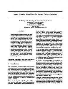
Connecting Element

'L' Joint

some error in the natural frequencies the mode shape correlation is very good. The model of the frame will be updated using generic parameters. The generic model updating approach is based on the idea of adjusting the mode shapes and natural frequencies of elements or substructures (Gladwell and Ahmadian, 1995). For example, a joint model that requires updating may be represented as a substructure. The mode shapes of the initial finite element model could be assumed correct, and the natural frequency of the first mode, typically a bending mode, could be updated. Thus the bending flexibility of the joint is changed to produce a model that better represents the measurements. The element mass matrices are assumed to be correct. The frame model consists of beam/bar elements, each of which has 3 rigid body modes and 3 strain modes. The strain modes have the form 0

0 0

13 Vo =

0 0

p

-p

0 0

0

~p

2