Grammar Constraints: Combining Expressiveness with Efficiency Serdar Kadioglu Brown University, Department of Computer Science P.O. Box 1910, Providence, RI 02912, U.S.A.
[email protected] Supervised by Prof. Meinolf Sellmann Abstract Constraints based on formal languages represent variables as a string to be derived from a given grammar. Such representations hold promise for solving combinatorial problems in scheduling and rostering. In this thesis, we devise a time-and space-efficient incremental arcconsistency algorithm for constraints based on context-free grammars. Our experiments on a shift-scheduling problem show massive speed-ups for the incremental algorithm compared to its non-incremental counterpart. We further compare our results against an alternative algorithm based on AND/OR decomposition.
1
Introduction
Constraint Programming (CP) is a very powerful technique for solving combinatorial problems. A key element contributing to this power are global constraints. Global constraints are intuitive modeling entities that combine common combinatorial structures with efficient filtering algorithms. One attractive mechanism to specify global constraints is via formal languages. The first constraint in this regard was based on regular languages [Pesant, 2003]. The incremental implementations of Regular were shown to perform very successfully on various problems and it was even used to replace custom constraints which can be expressed as regular languages [Pesant, 2003], [S.Bourdais, 2003]. Following the success of Regular, constraints based on grammars higher up in the Chomsky hierarchy are investigated. [Sellmann, 2006] and [Quimper and Walsh, 2006] theoretically study constraints based on context-free grammars and show that context-free grammar filtering can be done in polynomial time. [Quimper and Walsh, 2007] implement one such propagator for context-free grammar constraints. However, the method is impractical due to its cubic space requirements. In this thesis, we focus on practical aspects when dealing with context-free grammars. Our contribution is to devise a time-and space-efficient incremental arc-consistency algorithm. In particular, we improve the space efficiency of the context-free grammar propagator by a factor of n. 1
The rest of this thesis is structured as follows. Section 2 presents some preliminaries and notation on CP. Section 3 introduces grammar constraints. Section 4 describes our filtering algorithms. Section 5 compares the algorithms experimentally. Finally, in Section 6 we conclude our work.
2
Constraint Programming Preliminaries
We first introduce some basic constraint programming concepts. For more information we refer to [Apt, 2003]. A constraint satisfaction problem (CSP) P is a triple P =< X, D, C > where X is a n-tuple of variables X =< x1 , . . . , xn >, D is corresponding domains of variables D =< d1 , . . . , dn > such that xi ∈ di , ∀i ∈ 1 . . . n, and C is a set of constraints C = {c1 , . . . , ck } where each ck ∈ C specifies allowed combinations of values to a subset of the variables in X. Constraints of arity 2 are called binary constraints and constraints defined by an arbitrary arity are called global constraints. A constraint can be specified extensionally by a list of its satisfying tuples, although, it is intractable to enumerate all satisfiable tuples in practice. Global constraints are used to express ubiquitous patterns (e.g. a set of variables must take different values, notice that the size of the pattern is not fixed). It is important to incorporate global constraints in constraint solvers so that users can express such common patterns easily. However it is also important to have a way to propagate them without using generic arc consistency algorithms since optimal generic arc consistency algorithms require O(rdr ) time for constraints involving r variables with maximum domain size d. An assignment gives each variable a value from its domain and a solution is an assignment which satisfies all constraints. Broadly, constraint solvers apply two techniques to solve CSPs; inf erence and search and their various combinations. Inference is conducted via constraint propagation while a systematic search is performed to explore the finite search space Ω =⋊ ⋉i Di (where ⋊ ⋉ is the join operator relational algebra). The search process constructs a search tree by enumerating all possible variable-value combinations until we find a solution or prove that none exists while constraint propagation is applied at each node to reduce the exponential number of combinations. Constraint propagation removes domain values that do not belong to a solution with respect to a constraint. The removal of inconsistent values is called f iltering and the process is repeated for all constraints until no more domain values can be removed.
2
3
Global Constraints
A global constraint is a constraint that captures a relation between more than two variables. One of the best-known and probably the most influential global constraint is all dif f erent(x1 , ..., xn ) [R´egin, 1994], which specifies that a set of variables x1 , ..., xn should be assigned to distinct values. A global all dif f erent constraint might seem redundant in the sense that the same relation can be expressed semantically equivalently by a conjunction of quadratic number of binary inequality constraints. However, global constraints not only help in compact representations but they also facilitate the work of the constraint solver by providing it with a better view of the problem. For instance, let us compare all dif f erent(x1 , x2 , x3 ) versus x1 6= x2 & x2 6= x3 & x3 6= x1 over domains D(X) = {1, 2}. The all dif f erent constraint immediately prunes the domains and returns a failure whereas the binary constraints are not capable of removing any value since they check only two variables at a time, hence depend on branching to conclude a failure. In short, the importance of global constraints is twofold; first they are expressive and intuitive units of modeling, and second they yield stronger propagation as they capture larger problem structure.
3.1
Grammar Constraints
We will consider global constraints which are specified in terms of formal languages that accept valid assignments for a sequence of n variables. Such constraints hold promise for solving combinatorial problems in scheduling and rostering problems to ensure that certain patterns do or do not occur over time. For example, we may wish to ensure that anyone working four consecutive shifts then has a break or lunch. Such a specification can be expressed easily by a grammar. The first constraint based on formal languages was for regular languages [Pesant, 2003]. Regular languages are precisely those accepted by a deterministic finite automaton. One natural limitation of regular constraint is that some languages (e.g. correctly bracketed expressions) can not be specified with a deterministic finite automaton that is polynomial in size. We move above regular languages and consider constraints based on context-free languages. Context-free languages are exactly those languages accepted by non-deterministic pushdown automaton. Formally; Definition 1. Context-Free Grammars A grammar is a tuple G = (Σ, N, P, S0 ) where Σ is the alphabet, N is finite set of non-terminals, P ⊆ (N ∪ Σ)∗ N (N ∪ Σ)∗ × (N ∪ Σ)∗ is the set of productions and S0 ∈ N is the start symbol. The grammar G and the language LG are context free given that P ⊆ N x(N ∪ Σ)∗ .
3
Any context-free grammar can be written in Chomsky Normal Form (CNF) in which each rule yields either just one terminal or two non-terminals. For a full introduction on formal languages we refer the interested reader to [Hopcroft and Ullman, 1979]. Now, we review the definition of context-free grammar constraints from [Sellmann, 2006]. Definition 2. Context-Free Grammar Constraints For a given grammar G = (Σ, N, P, S0 ) and variables X1 , . . . , Xn with domains D1 := D(X1 ), . . . , Dn := D(Xn ) ⊆ Σ, we say that GRAM M ARG (X1 , . . . , Xn ) is true for an instantiation X1 ← w1 , . . . , Xn ← wn if and only if it holds that w = W1 . . . wn ∈ LG ∩ D1 × · · · × Dn . We denote a given grammar constraint GrammarG (X1, . . . , Xn ) over a context-free grammar G in CNF by CF GCG (X1 , . . . , Xn ).
4
Context-Free Grammar Filtering
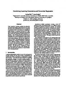
[Sellmann, 2006] presents a filtering algorithm for CFGC which is based on the Cooke, Younger, Kasami (CYK) parsing algorithm. Given a word of size n, let wij denote the sub-sequence of letters starting at position i with length j. Based on a grammar G(Σ, N, P, S0 ) in Chomsky Normal Form, CYK determines iteratively the set Si,j of all non-terminals from where we can derive wij for all 1 ≤ i ≤ n and 1 ≤ j ≤ n − i. It is easy to initialize the sets Si1 just based on wi and all productions (A → wi ) ∈ P . Then, for j from 2 to n and i from 1 to n − j + 1, we have that Sj−1 Sij = k=1 {A | (A → BC) ∈ P with B ∈ Sik and C ∈ Si+k,j−k }. Then, the word is in the language defined by the grammar G if and only if S0 ∈ S1n . From the recursion equation it is simple to derive that CYK can be implemented to run in time O(n3 |G|) = O(n3 ) when we treat the size of the grammar as a constant. The filtering algorithm works bottom-up by computing sets Sij for increasing j after initializing Si1 with all non-terminals that can produce in one step a terminal in the domains of Xi . Then, the algorithm works top-down by removing all non-terminals from each set Sij which cannot be reached from S0 ∈ S1n . Example: Assume we are given the following context-free, normal-form grammar G = ({], [}, {A, B, C, S0 }, {S0 → AC, S0 → S0 S0 , S0 → BC, B → AS0 , A → [ , C → ] }, S0 ) that gives the language LG of all correctly bracketed expressions (like, for example, “[[][]]” or “[][[]]”). In Figure 1, we illustrate how our algorithm works when the initial domain of X3 is D3 = {[} while all other domains are D1 = D2 = D4 = {[, ]}. First, we work bottom-up, adding non-terminals to the sets Sij if they allow to generate a word in Di × · · · × Di+j−1 . We initialize the first row, Si1 , with all non-terminals that can produce in one step a terminal in the domain of Xi . Then, in the second step, we work top-down and remove all non-terminals that cannot be reached from 4
Figure 1: Overview of CFGC filtering
5
S0 ∈ S1n . Note that, each node in Sij corresponds to a non-terminal in the grammar and each edge is a part of a production rule. For example, the non-terminal S0 in cell S12 is derived from the production S0 → AC using nodes A and C from S11 and S21 , respectively, and helps producing S0 in S14 together with S0 in S32 . We see that the constraint filtering algorithm determines “[ ][ ]” as the only word in LG ∩ D1 . . . D4 . In [Sellmann, 2006], it was shown: Theorem 4.1. CYK based filtering algorithm achieves generalized arc-consistency for the CF GC and requires time and space cubic in the number of variables.
4.1
A Memory- and Time-Efficient Filtering Algorithm
Theorem 4.1 states a theoretical algorithm for filtering grammar constraints that can run in polynomial time. From a practical point of view, cubic runtime per propagation is prohibitive. [Quimper and Walsh, 2007] implemented a propagator which is based on decomposition of the above outlined CYK structure into AND/OR nodes. The decomposition runs incrementally faster in cubic time. However, the method is impractical even for small sized instances due to its excessive cubic memory requirements. In this section, we show how to improve the space efficiency of the context-free grammar propagator and we outline an algorithm that combines highly incremental behavior with quadratic space requirements. One way to speed up filtering algorithms is to incorporate mechanism to incrementally update important data structures. In fact, the filtering algorithm is often applied with slightly changed domain information. Therefore, it is desirable that the data structures built during the first filtering operation are maintained dynamically without building them again for each subsequent run. Our incremental algorithm for CFGC filtering works as follows. In Figure 1 we observe that the algorithm first works bottom-up, determining from which non-terminals of the grammar we derive a legal word. Then, it works top-down determining which non-terminal nodes can be used in a derivation that begins with start symbol S0 ∈ S1n . In order to save both space and time, we will modify these two steps such that every non-terminal in each set Sij will perform just enough work to determine whether its respective node will remain in the shrunken graph. To this end, in the first step that works bottom-up we need a routine that determines whether there exists a support from below: That is, whether a node has any outgoing arcs. Analogously, in the second step that works top-down we need a routine that checks whether there exists a support from above: That is, whether a node has any incoming arcs.
6
The challenge is to avoid having to pay with time what we save in space. To this end, we need a methodology which prevents us from searching for supports (from above or below) that have been checked unsuccessfully before. Very much like the well-known arc-consistency algorithm AC-6 for binary constraint problems [C. Bessiere, 1993] we achieve this goal by ordering potential supports so that, when a support is lost, the search for a new support can start right after the last support, in the respective ordering. That is; we generate at most one non-terminal in any Sij cell. In [Kadioglu and Sellmann, 2008] we show: Theorem 4.2. For a sequence of s monotonically tightening context-free grammar filtering problems, based on the grammar G in CNF, filtering for the entire sequence can be performed in time O(n3 |G|) and space O(n2 |G|). Example: Consider our previous example of correctly bracketed expressions with four variables each with a domain {[, ]}. In Figure 2 we show how the incremental algorithm constructs the necessary structure and in Figure 3 we show how it maintains it in case of a domain change. While a non-incremental algorithm would disregard the previous structure and build a structure from scratch, incremental algorithm modifies only the necessary parts.
j 4 3
j S0 B
B S0 S0
2 1
4 3 S0
C A C A C A C A 1
2
3
4
S0 B
2
S0 S0
1
A C A C A C
i
1
2
S0
3
4
i
Figure 2: The initial data structure is identical to the non-incremental case. The figure on the left works bottom-up and the figure on the right works top-down. Left and right parenthesis are removed from the domain of the first and the last variable respectively.
j 4
S0
3 2
S0
S0
1
A C
A C
1
2
3
4
i
Figure 3: When the left parenthesis (labeled as #1) is removed from the domain of the third variable the incremental algorithm propagates the effect of the removal up (#2) and then down (#3).
7
It should be noted that Theorem 4.2 achieves quadratic space for a sequence of s monotonically tightening context-free grammar filtering problems. In order to handle backtracks, we need to store lost supports for each removed node. Consequently, within a full backtrack search we cannot keep the claim of quadratic space requirements. However, as we will see in the next section, the amount of additional restoration information needed is fortunately very limited in practice.
4.2
Handling Backtracks
In the non-incremental algorithm, the data structure is created from scratch for every decision point which saves us from dealing with an explicit backtrack operation. However, in the incremental case only a subpart of the original structures is changed, hence we need a way to undo the changes that we have committed and to restore back to a previous state. This is possible by storing extra information whenever a node is removed from any Sij (notice that domain filtering monotonically decreases the number of nodes in S). In fact, we do not have to store a node as a whole but only the necessary information to create it again. A node can be created given its position i, j and the production rules that were supporting it from above and below together with their splitting indices. This information is stored in an array called T racer. A pointer, called marker is used to refer to the most recent removals. Each time a branching decision is made, the marker is increased. The backtrack method operates on an index of the T racer pointed by the marker: T racer[marker]. The method considers changes in reverse order and re-creates removed nodes using their stored information. In Figure 4 we give a snapshot of the T racer and the marker following the domain change in Figure 3.
Figure 4: As the nodes are removed backup information is stored in Tracer. At each decision point the marker is shifted to the right. When backtrack is invoked the nodes in T racer[marker] is re-created and the marker is shifted to the left.
5
Experimental Results
Our experiments are on real-world instances of the shift-scheduling problem introduced in [S. Demassey, 2006]. The problem is that of a retail store manager who needs to staff his employees such that the expected demands of workers for various activities that must be performed at all times of
8
Benchmark ID
11 12 13 14 15 16 17 18 19 1 10 21 25 26 27 28 29 2 10
Search-Tree
Non-Incremental
Incremental
Speedup
#Act #Workers #Fails #Prop’s #Nodes Time[sec] Mem[MB] Time[sec] Mem[MB]
1 1 1 1 1 1 1 1 1 1 2 2 2 2 2 2 2
1 3 4 5 4 5 6 2 1 7 2 4 5 6 2 1 7
2 144 409 6 6 6 5311 6 2 17447 10 24 30 44 24 16 346
136 577 988 749 598 748 6282 299 144 19319 430 412 603 850 363 252 1155
19 290 584 191 137 161 5471 99 35 1769 65 100 171 158 114 56 562
79 293 455 443 399 487 1948 193 80 4813 359 355 496 713 331 220 900
12 38 50 60 50 60 72 26 16 82 44 44 58 84 44 32 132
1.75 5.7 8.12 9.08 7.15 9.1 16.13 3.57 1.71 25.57 7.34 7.37 9.89 15.14 3.57 4.93 17.97
24 80 106 124 104 132 154 40 18 176 88 88 106 178 84 52 160
45 51 56 46 55 53 120 54 47 188 49 48 50 47 92 44 50
Table 1: Shift-scheduling: We report running times on an AMD Athlon 64 X2 Dual Core Processor 3800+ for benchmarks with one and two activity types. For each worker, the corresponding grammar in CNF has 30 non-terminals and 36 productions. Column #Propagations shows how often the propagation of grammar constraints is called for. Note that this value is different from the number of choice points as constraints are usually propagated more than just once per choice point. the day are met. Problem details and labor regulations can be found in [Kadioglu and Sellmann, 2008]. Table 1 summarizes the results of our experiments. We see that the incremental propagation algorithm vastly outperforms its non-incremental counterpart, resulting in speed-ups of up to a factor 188 while exploring identical search-trees! It is quite rare to find that the efficiency of filtering techniques leads to such dramatic improvements with unchanged filtering effectiveness. We also tried to use the decomposition approach from [Quimper and Walsh, 2007], but, due to the method’s excessive memory requirements, on our machine with 2 GByte main memory we were only able to solve benchmarks with one activity and one worker only (1 1 and 1 9). On these instances, the decomposition approach implemented in Ilog Solver 6.4 runs about ten times slower than our approach (potentially because of swapped memory) and uses about 1.8 GBytes memory. Our method, on the other hand, requires only 24 MBytes. Finally, when comparing the memory requirements of the non-incremental and the incremental variants, we find that the additional memory needed to store restoration data is very limited in practice.
9
6
Conclusion
We devised an incremental space- and time-efficient arc-consistency algorithm for context-free grammar constraints. For an entire sequence of monotonically tightening problems, we can now perform filtering in quadratic space and the same worst-case time as it takes to parse a context-free grammar by the Cooke-Younger-Kasami algorithm (CYK). We showed experimentally that the new algorithm is equally effective but massively faster in practice than its non-incremental counterpart. We also showed that our memory requirements are within practical limits in contrary to the existing AND/OR decomposition approach. Context-free grammar constraints have been made available in the Cornflower Library which can be found online at http:://www.cs.brown.edu/research/cornflower. Both incremental and non-incremental filtering algorithms can be used as an extension to Ilog Solver or as a stand-alone C++ application.
References K.R. Apt. Principles of Constraint Programming. cambridge Univ. Press, 2003. M.O. Cordier C. Bessiere. Arc-Consistency and Arc-Consistency again. AAAI, 1993. J.E. Hopcroft and J.D. Ullman. Introduction to Automata Theory, Languages and Computation. Addison Wesley, 1979. S. Kadioglu and M. Sellmann. Efficient Context-Free Grammar Constraints. AAAI, AAAI Press, pp. 310-316, 2008. G. Pesant. A Regular Language Membership Constraint for Sequences of Variables. Modelling and Reformulating Constraint Satisfaction Problems, pp. 110–119, 2003. C.-G. Quimper and T. Walsh. Global Grammar Constraints. CP, LNCS 3258:751–755, 2006. C.-G. Quimper and T. Walsh. Decomposing Global Grammar Constraints. CP, LNCS 4741:590–604, 2007. J.-C. R´egin. A Filtering Algorithm for Constraints of Difference in CSPs. AAAI, AAAI Press, pp. 362-367, 1994. L.-M. Rousseau S. Demassey, G. Pesant. A Cost-Regular Based Hybrid Column Generation Approach. Constraints, 11(4):315–333, 2006. 10
G.Pesant S.Bourdais, P.Galinier.
HIBISCUS: A Constraint Programming Application to Staff
Scheduling in Health Care. CP, LNCS 2833:153-167, 2003. M. Sellmann. The Theory of Grammar Constraints. CP, LNCS 4204:530–544, 2006.
11


![[PDF] Download Grammar for Sentence Combining Full Online ...](https://m.moam.info/img/260x300/pdf-download-grammar-for-sentence-combining-full-o_6478914c097c4786708cf77c.jpg)

![[PDF] Download Grammar for Sentence Combining Full Online ePub](https://m.moam.info/img/260x300/pdf-download-grammar-for-sentence-combining-full-o_6478908c097c474d228d4ae8.jpg)

